



Abstract
A thin-film magneto-impedance (MI) sensor has the unique property of step-like magneto-impedance change, in the case where the sensor has an in-plane uniaxial inclined easy axis. A domain observation shows that the step-like change is due to a magnetization transition within three states, such as longitudinal single domain with parallel state, the one with anti-parallel state and the inclined Landau-Lifshitz domain (ILLD). In a condition where the sensor has an easy axis of 70 degrees relative to the short side axis of the rectangular element, the transition is limited between the parallel and anti-parallel in spite of existing of stable ILLD. This paper reports a trial of control the magnetization transition from the single domain state to the ILLD state by controlling a normal field with canted angle distribution along the element position, which is aiming for realizing a low energy consumption sensor with inextinguishable memory function using a phenomenon of a magnetic domain transition for the use of sensor network.
Introduction
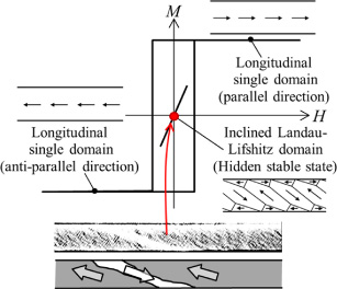
A magneto-impedance (MI) element with a stepped impedance property was obtained for amorphous Co85Nb12Zr3 soft magnetic rectangular thin film with an in-plane uniaxial easy axis in a direction of nearly 60 degrees relative to the short-side axis [1]. The stepped change of impedance occurs simultaneously with the appearance or the disappearance of a certain magnetic domain, specifically the in-plane inclined Landau-Lifshitz-domain (ILLD), changing into or from a single domains with longitudinal + or − momentum direction (LSD+, LSD−). The physical basis of the change of magnetic domain was explained by the relationship of magnetic energy between in-plane inclined Landau-Lifshitz-domain, and a single domain with longitudinal magnetic momentum [2]. The element with these three domain states co-existing stably around zero external magnetic fields was realized by controlling the direction of easy axis, and is expected for sensor application [3]. The existence of hidden, but energetically stable state, was predicted by theoretical analysis. Two kind of approach was carried out for the analysis. One is the analysis of magnetic energy for the in-plane inclined Landau-Lifshitz-domain (ILLD) and longitudinal single domain (LSD) with introduction of asymmetrical threshold barrier [4,5], another is the analysis using a simplified domain structure model [6]. Both of these analyses predicted the existence of hidden stable domain state for the element in which there is an easy axis in a certain direction. An experimental study on reconstructing the hidden ILLD state originating from a single domain was reported by controlling a canted distributed normal field [7,8]. A domain simulation using the assembled domain structure model (ADSM) also showed that controlling the degree of canted distribution of the normal field could reconstruct the hidden ILLD state [9]. To help convey the aim of this study, a schematic explanation of the hidden state in a MH diagram coinciding with a impedance variation is shown in Fig. 1. In this paper, a trial of control the magnetization transition from the single domain state to the hidden ILLD state by controlling a normal field with canted angle distributed along the element position is reported.
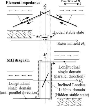
Schematics of element impedance and MH diagram with hidden state.
Experimental procedure
The element was fabricated by a thin film process. An amorphous Co85Nb12Zr3 film was RF-sputter deposited onto a soda glass substrate and then micro-fabricated into rectangular elements by a lift-off process. The dimensions of the element are 2000 μm long, 20 μm wide, 1.6 μm thick. The element was annealed in a magnetic field to induce uniaxial magnetic anisotropy. The direction of the magnetic anisotropy was controlled by the direction of the magnetic field while annealing. In this study, the magnetic field during annealing, 240 kA/m in 673 K, was oriented in 71 degrees relative to the short-side axis of the element. For the element made by this process, the saturation magnetization was 0.93 T and the anisotropy field was 480 A/m.
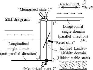
Schematic of a M-H diagram and related magnetic domains for the element having a hidden state with indicating both the memorized and the reset state.
Figure 2 shows a schematic of MH diagram of fabricated element which has a uniaxial easy axis in an in-plane inclined direction, 71 degrees relative to the short-side axis of the element. In this case, the element is expected to have a hidden ILLD state. A “Memorized state” is determined here as a state where the in-plane external field is zero (H x = 0) and the domain is parallel or anti-parallel single domain state. A “Reset state” of the proposed three states memory sensor is defined as the hidden ILLD state. When a sensing field which is larger than a certain threshold value along the in-plane longitudinal direction is applied, the reset state changes to the memorized state and be kept it. The aim of this study is to realize a controlled magnetization transition which changes the single domain state into the “hidden” ILLD state, that is to say reset the memorized state to the reset state
The experiment was carried out by applying a strong magnetic field with constant value along the normal direction of the substrate plane using an apparatus made by a certain structure of NdFeB magnets. It is possible to control the distributed canted angle relative to the normal direction within the applied normal field. An in-plane bias magnetic field could also be controlled by using a Helmholtz coil for measuring a variation in the element domain as a function of in-plane magnetic field. This in-plane field was applied along the length direction, which is the sensing direction, of the rectangular shape element.

Schematic of applied magnetic field with distributed normal field.
Figure 3 shows a schematic of the distributed normal field. An equation of the vector of the normal field, B
normal
, is shown as follows;
In this study, the following were assumed;
These assumptions represent a field that has a linearly varied X-directional component within the constant normal field B z .
In this study, a magnetic flux density B is derived from B = 𝜇0 H, where 𝜇0 is the permeability of free space. Therefore the expression B is obtained from the magnetic field in free space.
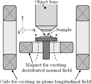
Schematics of the measurement system.
Figure 4 shows a schematic of the measurement system. The domain structure was observed by a Kerr microscope. The normal magnetic field and the in-plane magnetic field were controlled individually on the observation stage of the Kerr microscope. An applied value of the normal field, B z , as well as the distributed field, ΔB x ∕Δx, can be controlled by using the normal field generating ring-shaped magnet. The magnetic field in in-plane sensing direction of the element is controlled by the Helmholtz coil. The distributed field, ΔB x ∕Δx, on the observation-stage of the Kerr microscope was controlled by the vertical position of the ring-shaped magnet. The variation of the vertical position of this magnet changes slightly the B z value on the observation-stage. On the other hand, it changes the ΔB x ∕Δx, therefore it is controllable by changing the Z-position of the ring-shaped magnet.
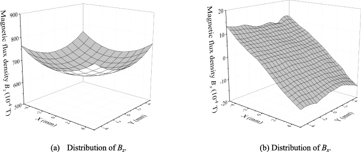
Example of simulated magnetic field on substrate surface.
An example of the distribution of magnetic field, which is generated by the apparatus of Fig. 4, is shown in Fig. 5. The field is a result of 3-dimensional (3D) FEM simulation. Figure 5a shows a distribution of B z on the horizontal plane lying at z = −0.5 mm. Here the center of the ring-shaped magnet, shown in Fig. 4, is defined as z = 0, and it is a position where ΔB x ∕Δx = 0. The variation of B z was almost 12% within a range of ±2 mm of X–Y plane, here, the central value of B z was 64.0 mT (640 G). Figure 5b shows a distribution of B x on the same plane, with the same area of the X–Y plane as in Fig. 5a. The figure shows a canted flat plane of variation. From some simulations in other Z-positions, the inclination of distributed field ΔB x ∕Δx, was almost a constant value, and it is possible to control the value by changing the vertical position of the measurement plane. In this figure, the z value was chosen as negative value for the reason of visual expression in Fig. 5b. The sign of ΔB x ∕Δx for z > 0 must be positive, because the apparatus is symmetrical on the X–Y plane.
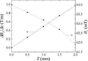
Relationship between the z position in the ring-magnet and both the B z and the ΔB x ∕Δx.
Figure 6 shows a relationship between the z position in the ring-magnet and both the B z and the ΔB x ∕Δx. The horizontal axis in this figure represents z value, the vertical right axis represents B z , and the vertical left axis represents ΔB x ∕Δx. These relationships are estimated by 3D-FEM magnetic field simulation. The ΔB x ∕Δx = 0 is obtained for z = 0, and the ΔB x ∕Δx = 0.4 T/m is obtained for z = 0.8 mm. The value of z in the following experiment was ranging from z = 0 to z = 0.7 mm. In this study, the B z value in the central area is 64.0 mT, and the variation according to the control of Z -position was lower than 1.2%.
Concerning the variation of magnetic field in the Y-direction, ΔB y ∕Δy has almost the same value as ΔB x ∕Δx because the symmetry of the ring magnet shape. However it is negligible owing to the narrow width of this element (20 μm) in this study.
In this subsection, an observed magnetic domain transition of an element which has easy axis at 71° is shown. This is almost the same condition as the previous report which shows an experimental expectation of the existence of hidden ILLD state [7,8]. The observation of the magnetic domain was carried out by observing a central part of the rectangular element.
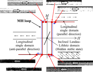
Typical variation of magnetic domain for the element with easy axis in 71 degrees.
When the normal field B z = 64 mT and the distributed parameter ΔB x ∕Δx = 0, that is obtained by the condition z = 0 in Fig. 6, the domain transition of this element was limited between longitudinal parallel and anti-parallel state, when the longitudinal applied field varies. The longitudinal direction is the sensing direction of the sensor. Figure 7 shows a typical variation of magnetic domain. The horizontal axis represents a longitudinal magnetic field which was controlled by the Helmholtz coil of in-plane longitudinal direction. In this figure, some observed domain pictures are shown with each pointed arrow on a point of an expected magnetization curve. The observed magnetic field of negative single domains, the bottom side pictures, were −84.4 A/m (−1.06 × 10⁻⁴ T), −46.2 A/m (−0.58 × 10⁻⁴ T), 16.7 A/m (0.21 × 10⁻⁴ T) and 43.8 A/m (0.55 × 10⁻⁴T) respectively. And the ones for positive single domains, the upper side pictures, it was −44.6 A/m (−0.56 × 10⁻⁴ T), −8.8 A/m (−0.11 × 10⁻⁴ T), 44.6 A/m (0.56 × 10⁻⁴ T) and 67.6 A/m (0.85 × 10⁻⁴ T) respectively. In the case of the increasing magnetic field, the domain transition occurs at about 43.8 A/m (0.55 × 10⁻⁴ T). And in the case of decreases, it occurs at about −45.4 A/m (−0.57 × 10⁻⁴ T).
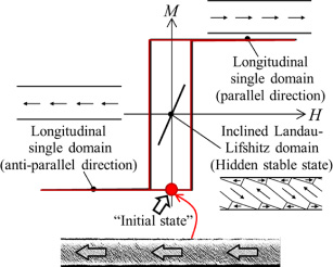
Initial state of the following trial of multi-domain reconstruction.
Figure 8 shows an initial state of the following trial of multi-domain reconstruction. It is the single domain state in the negative direction, and the external field condition is as follows; the normal field and the distributed field is as the same as Fig. 7, B z = 64 mT and ΔB x ∕Δx = 0, and the in-plane field applied to the element’s longitudinal direction was H x = 0.
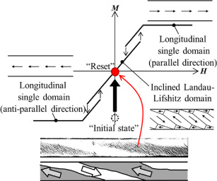
Magnetic domain with application of distributed field ΔB x ∕Δx = 0.24 T/m.
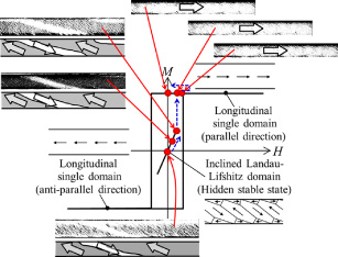
For the purpose of re-constructing the multi-domain state originated from the single domain state of Fig. 8, The distributed field was changed by controlling the Z-position of the ring-shaped magnet. In Fig. 9, the ring-shaped magnet was moved down and the relative position of the observed element was z = 0.6 mm. In this case, the distributed parameter ΔB x ∕Δx was 0.24 T/m. The magnetization curve in Fig. 9 is an expected one based on the result of refs [8,9]. An appearance of multi-domain state, which was assumed as the ILLD state, was experimentally observed. For the domain picture is not clear, illustration is shown below it.
Magnetic domain after application of ΔB x ∕Δx = 0.24 T/m and return to ΔB x ∕Δx = 0.
After the multi-domain reconstruction occur, the distributed field returns to ΔB x ∕Δx = 0, by changing the Z-position of the ring-shaped magnet to the initial position z = 0 with keeping H x = 0. The result shows that the multi-domain state had been kept despite the magnet movement procedure. It is shown in Fig. 10. In this figure, the picture of magnetic domain was illustrated below it, for the clear understanding of the observed domain pattern. It was obtained that the multi-domain state had been kept even if the distributed field returned to ΔB x ∕Δx = 0. It is expected that the domain state changes into hidden stable ILLD state.
Variation of magnetic domain after reconstruction of multi-domain ILLD state.
After the sequential procedure of reconstructing multi-domain state, above mentioned, the in-plane magnetic field was varied and then the variation of magnetic domain was observed. Figure 11 shows the result of this experiment. Here, the normal field B z = 64 mT and the distributed parameter ΔB x ∕Δx = 0. Starting from the multi-domain state around H x ≈ 0, the external field gradually increases, and when the external field exceeds 31.0 A/m (0.39 × 10⁻⁴ T) the domain state suddenly changes to single-domain state. The observed three points in the hidden ILLD state in this figure was around 0, 22.3 A/m (0.28 × 10⁻⁴ T) and 30.2 A/m (0.38 × 10⁻⁴ T) respectively. The domain picture which is just changed from the multi-domain to the single domain was 31.8 A/m (0.40 × 10⁻⁴ T). After the domain transition to the single domain, the external field increased to 42.2 A/m (0.53 × 10⁻⁴ T) and then decreased to ≈ 0. Compared with Fig. 7 which is the original two-state transition phenomena, the value of largest external field in the Fig. 11 was lower than the transition external field 43.8 A/m (0.55 × 10⁻⁴ T) in Fig. 7. In case of Fig. 11, the applied in-plane field was lower than the domain transition field 43.8 A/m. The observed three points in the positive single domain state in this figure was around 0, 31.8 A/m (0.40 × 10⁻⁴ T) and 42.2 A/m (0.53 × 10⁻⁴ T) respectively. The multi-domain state had been changed to the single-domain state, and the single-domain was kept when the external field returned to H x ≈ 0.
The application of a normal field with canted distribution has the effect of controlling the appearance of the in-plane inclined Landau-Lifshitz-domain state for the stepped MI element. In this study, an experimental confirmation were carried out for reconstructing multi-domain state, that would be the hidden ILLD state, originated from single domain state. The magnetic field B z = 64 mT was applied as the constant normal field, and the ratio of distribution, ΔB x ∕Δx, was controlled from 0.0 T/m to 0.24 T/m. The element which was used in this experiment had a property of domain transition between the positive single-domain and the negative one in the condition of without application of the normal field. It is expected that this element has the hidden ILLD state. The appearance of ILLD multi-domain state can be accomplished by controlling the distributed field. The domain control procedure is as follows; as increasing the distributed field ΔB x ∕Δx with keeping B z as a same value and also with keeping H x ≈ 0, the appearance of the ILLD multi-domain state can be confirmed at a certain value of ΔB x ∕Δx. After the appearance of ILLD multi-domain state is observed, the distributed field ΔB x ∕Δx controls back to zero. Then the hidden ILLD multi-domain state is reconstructed. After accomplish this “rest” procedure, an external field in the sensing direction which is larger than the threshold value would be applied, then the multi-domain state vanishes and get to be a longitudinal single-domain “memorized” state. The point which must be mentioned especially is that the main effect on reconstruction of multi-domain state is the distributed parameter ΔB x ∕Δx.
The demagnetizing field in the thickness direction of the thin film element in this study is expected to be large enough to compensate the external normal field applied to the element. There are some previous studies which deduce a formula calculating it for magnetic bodies with various shapes. Based on Ref. [11] and Ref. [12], a demagnetizing coefficient in the thickness direction D z is calculated for the same shape of element as this study, such as thousands of micro-meters length, tens of micro-meters width and several micro-meters thickness. It deduced as D z = 0.897 in the both Refs. Based on our element’s saturation magnetization I s = 0.93 T and soft magnetic property, a component of magnetization in Z-direction I z in the normal field is roughly estimated as I z ≈ 0.062 ⋅ I s for the value of applied normal field 64 mT. The effect of the normal field based on the consideration of demagnetizing field and of rotation of magnetic moment towards Z-direction for the domain transition phenomenon is our future subject of study. But in this study, there would be a certain effect on a formation of magnetic domain, because the observed ILLD domain pattern has been distorted and it is not a clear ILLD but a distorted multi-domain stripe pattern. In the previous study, ref [8], the domain control forced by ΔB x ∕Δx would be possible in a lower value of B z condition. It would be expected that an investigation using a low B z condition makes an exact and clear ILLD reconstruction for this phenomenon.
Summary
An existence of distributed canted angle relative to normal direction within the applied normal field can control the reconstruction of in-plane inclined Landau-Lifshitz-domain (ILLD) state originated from the single domain state for the stepped MI element with the hidden state. In this study, an actualization of memorize and reset operation of the stepped magneto-impedance sensor with hidden state is experimentally shown by controlling the degree of distribution of canted normal field applied to the element. The reset transition happens when the distributed field ΔB x ∕Δx is larger than 0.24 T/m was applied.
Footnotes
Acknowledgements
This work was supported by Nationwide Cooperative Research Projects by the Research Institute of Electrical Communication, Tohoku University. The author’s special thanks are due to Prof. Kazushi Ishiyama Tohoku University and also to Prof. Tetsuji Matsuo, Kyoto University for valuable discussion.