Consideration of magnetic saturation ECT using AC magnetisation

1. Introduction

We considered detections of microcracks in steel materials by eddy current testing (ECT) using a uniform eddy current probe [1–5]. In ECT of steel materials, the magnetic noise generated due to the variation of permeability in the test object limits the signal-to-noise (S∕N) ratio of the detection result. Therefore, magnetic noise reduction is especially important for microcrack detection. Thus, a technique called magnetic saturation ECT, which involves magnetisation of the test object, is considered to reduce the magnetic noise. Direct-current (DC) magnetisation is generally used for magnetic saturation ECT [6–9]; however, thick test objects cannot be magnetised suff iciently and demagnetisation might be necessary after flaw detection when using this approach.

Magnetic saturation ECT using alternating-current (AC) magnetisation was considered in this study to overcome these drawbacks. This approach changes the magnetisation state of the test object temporally. The detection results obtained for different synchronous positions (conditions) of the AC magnetisation and ECT were evaluated and compared to identify the optimum position. In addition, the magnetisation distribution in a test object was evaluated with a finite element method (FEM) analysis and the flaw detection results were verified.

2. Flaw detection and magnetisation method in ECT

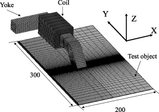
Figure 1 shows the magnetic saturation ECT system. Six test objects were prepared from an SPCC cold-rolled steel sheet (300 mm × 400 mm × 1 mm^t) with cracks (5.8 mm long and 100 μm wide) of different depths (480, 400, 308, 213, 70 and 43 μm). A two-pole yoke-type magnetiser (Denshijiki Industry Co., Ltd: Um-5BF) was used for magnetisation required for magnetic saturation ECT. The number of coil turns on the magnetiser was 410. The direction of magnetisation was assumed to be parallel to the length of the crack. The frequency and the excitation current used for the AC magnetisation were 60 Hz (commercial frequency) and 3.18 A _0−peak, respectively. The frequency for flaw detection via ECT was 50 kHz. The probe was placed on a precision stage and scanned along the surface of the test object. The detection signal from the ECT probe was measured by an ECT equipment (Aswan ECT Co., Ltd: Multi-2000); and the X and Y components of the signals were obtained by the phase detection using the ECT equipment. The phase of the Y signal was delayed by 90° compared with the X signal. Figure 2 shows the AC magnetic flux waveform measured using a wound search coil as the yoke of the magnetiser. Synchronous positions (P1–P9) between the AC magnetisation and the ECT were varied and the corresponding readings at each synchronous position were evaluated, as shown in Fig. 2.

OPEN IN VIEWER

Fig. 1.

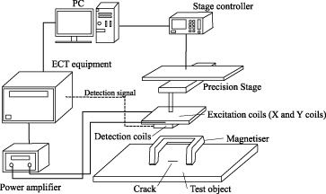
Magnetic saturation ECT system.

OPEN IN VIEWER

Fig. 2.

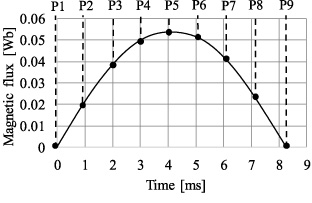
Synchronous positions of AC magnetisation and ECT.

Figure 3 shows the configuration of a multi-uniform eddy current probe. The probe comprised multi-detection coils (outer diameter: 2.2 mm, inner diameter: 1.2 mm, thickness: 0.7 mm and 140 turns) and two excitation coils (60 mm × 60 mm × 2 mm^t and 360 turns) around a Mn–Zn ferrite core. The excitation coils were composed of X and Y coils with orthogonal coil axes. Each excitation coil was excited independently. In the uniform eddy current probe, the excitation coils were placed in contiguity with the surface of the test object so that the uniform eddy current flowed in the same direction within the area of the detection coils. The coil axes of the excitation coils were arranged to be orthogonal to the direction of the coil axes of the detection coils, as shown in Fig. 3. Thus, the magnetic flux generated by the excitation coils was not directly measured by the detection coils.

OPEN IN VIEWER

Fig. 3.

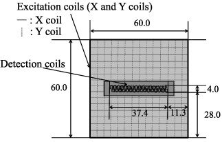
Configuration of probe.

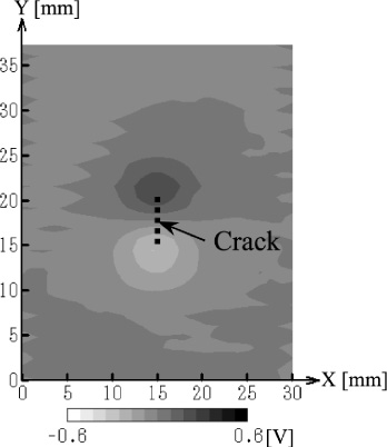
The detection results of a 300 μm-deep crack in synchronous positions P4 and P9 (as defined in Fig. 2) are shown in Figs 4 and 5. The phase of the ECT equipment was set such that the Y detection signal was at a maximum for each synchronous position. The Y signal around the cracks is shown as 2D contour figures. The dotted line shows the crack position. The eddy current during the ECT was assumed to be orthogonal to the length of each of the cracks. Therefore, positive and negative signals were recorded at each end of the crack. The detection signal in P9 was larger than that in P4 and the detection results were different for each of the other synchronous positions. Thus, flaw detection was evaluated for each synchronous position of the magnetisation and ECT and the optimum position was evaluated for magnetic saturation ECT using AC magnetisation.

OPEN IN VIEWER

Fig. 4.

Detection result in P4.

OPEN IN VIEWER

Fig. 5.

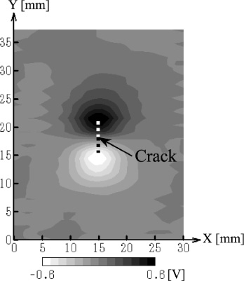
Detection result in P9.

Figure 6 shows the detection signal and noise. The detection signals in synchronous positions P1, P8 and P9 are large compared with those in P2–P7. Furthermore, the signal and noise in P8 are higher than those with the other positions. Figure 7 shows the S∕N ratios for each of the positions. The maximum S∕N ratios are obtained in P1 and P9. Therefore, we evaluated the sensitivity of the flaw detection system in P9.

OPEN IN VIEWER

Fig. 6.

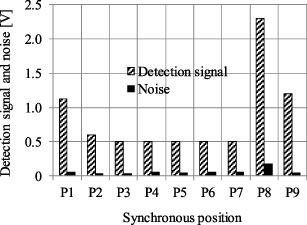
Detection signal and noise in each synchronous position.

OPEN IN VIEWER

Fig. 7.

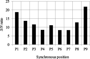
S∕N ratio in each synchronous position.

Figure 8 shows the S∕N ratio of the measurement of each crack depth and displays the detection results for the 70 and 43 μm-deep cracks. The S∕N ratio increases as the crack depth increases. A clear signal with S∕N ratio of 3.6 is obtained for the 70 μm-deep crack by magnetising the test object at the optimum synchronous position. However, no detection signal was observed for the 43 μm-deep microcrack. Thus, the limit of crack detection for the developed probe was 70 μm in depth.

OPEN IN VIEWER

Fig. 8.

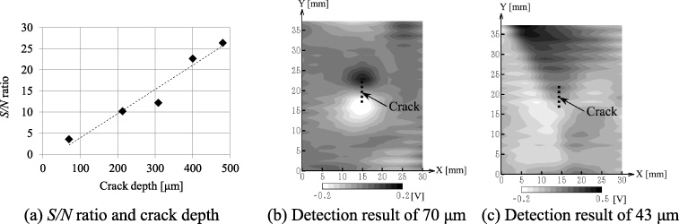
S∕N ratio and detection results in synchronous position P9.

The relationship between the magnetic flux in the test object, the synchronous positions and the detection results was evaluated in order to further investigate the results described above. Drill holes were jigged in the test object and a search coil was wound around the test object with 13 turns. The sectional area was 18 × 1 mm. Figure 9 shows the magnetic flux through the test object with each synchronous position with AC magnetisation. The magnetic flux density, which is equal to the magnetic flux divided by the sectional area of the search coil, was shown as a reference. The detection signal shown in Fig. 6 was then compared with the magnetic flux shown in Fig. 9. The test object is in a magnetic saturation state in P3–P7, which attenuated the record signal. The detection signals are different in P2 and P8 although the magnetic fluxes with these two positions were approximately equal. In P1 and P9, i.e., the optimum positions, the magnetic flux in the test object was nearly zero.

OPEN IN VIEWER

Fig. 9.

Magnetic flux in test object and synchronous positions.

With AC magnetisation, the magnetic flux varies between different depth positions in the test object owing to the phase difference generated in the magnetic flux according to the depth of the test object. However, from the measurements of the magnetic flux obtained using the search coil, the magnetic flux densities in the depth direction could not be determined. Therefore, the magnetic flux densities in test objects with different depths were evaluated via FEM analysis.

Figure 10 shows a transient-response FEM analysis (step-by-step method) model. The sizes of the magnetiser and the test object were modelled with the same parameters as in the experimental testing but the test object considered in the analytical model did not contain a crack. The test object was SPCC. The conductivity of the test object was 7. 5 × 10⁶ S∕m. A half-shape model was applied in order to consider the boundary area for efficient analysis. Because the yoke of the magnetiser was an electromagnetic steel sheet the conductivity of the yoke was set to zero to reproduce the lamination characteristic. The number of coil turns on the magnetiser and the excitation current were set to the same value as that used for the experimental testing. Figure 11 shows the B-H curves of the test object and yoke. A position at the inner size center of the magnetic pole in the magnetiser was evaluated.

OPEN IN VIEWER

Fig. 10.

Analytical model.

OPEN IN VIEWER

Fig. 11.

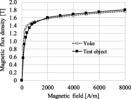
B-H curves of test object and yoke.

Figures 12(a), 12(b) and 12(c) show the magnetic flux density in the depth direction in synchronous positions P4, P8 and P9, respectively. The surface of the test object was set to Z origin. In P4, the test object is magnetised equally in the depth direction of the test object. In contrast, the magnetic flux density in the depth direction is different in P8 and P9. In P8, the magnetic flux density at the surface decreases although it is large at deeper positions. Therefore, by measuring the magnetic flux at a deep position in the test object, it was confirmed that a large magnetic flux was obtained, as shown in Fig. 9. The direction (phase) of the magnetic flux density varies within the test object in P9. Thus, the magnetic flux, as shown in Fig. 9, diminished because the magnetic flux density at each position was offset to some degree.

OPEN IN VIEWER

Fig. 12.

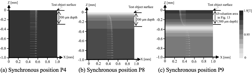
Magnetic flux density in depth direction.

Therefore, the magnetic flux density was evaluated as a function of depth for each synchronous position. In this study, the skin depth of the eddy current for ECT (50 kHz) was about 60 μm. However, the eddy current was distributed at the bottom of the crack. Thus, the magnetic flux density was evaluated within the region, including a depth of 300 μm below the skin depth. Figure 13 shows the line distribution of the magnetic flux density in the depth direction for each synchronous position (magnetic flux densities to the right direction in Fig. 12 was taken as positive values). In positions P1 and P9, the magnetic flux density decreases at the undersurface of the test object but a large magnetic flux density is observed at the surface. Large, uniform magnetic flux densities in the depth direction are simulated for P2–P7. In P8, the magnetic flux density at the surface is low, though a large magnetic flux density is observed at the undersurface.

OPEN IN VIEWER

Fig. 13.

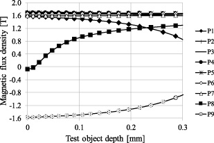
Magnetic flux density in depth direction for each synchronous position.

The relationship between the noise in the detection results and the magnetic flux density was also characterised, as shown in Fig. 6 and Fig. 13. According to the results, the magnetic noise increased with the permeability variation because the magnetic flux density was low at the surface of the test object in P8. Therefore, the noise of the detection result reported in Fig. 6 was the maximum. In except P8, because the enough magnetic flux density was provided at the surface of the test object, the noise of the detection results was decreased.

In addition, the relationship between the detection signal and the magnetic flux density was assessed. According to the results shown in Fig. 13, large magnetic flux densities were generated in P2–P7. Thus, the detection signal as well as the eddy current at the surface of the test object decreased owing to the decrease in the permeability and increase in the skin depth. In contrast, the eddy current increased because the magnetic flux density at the surface was low and the skin depth was shallow in P8, as shown in Fig. 13. Therefore, as shown in Fig. 6, the maximum detection signal was recorded in P8. In P1 and P9, since the magnetic flux density at the undersurface decreased compared with those in P2–P7, as shown in Fig. 13, the permeability did not decrease. Thus, the eddy current at the surface increased compared with those in P2–P7. Furthermore, the detection signals recorded in P1 and P9 increased compared with those in P2–P7. Consequently, synchronous positions P1 and P9 represent the optimum positions.

Herein, we investigated magnetic saturation ECT using AC magnetisation wherein the magnetisation state in the test object changed temporally. Therefore, synchronisation of the AC magnetisation and the ECT was considered and the detection results were evaluated under different synchronous positions. The results showed that the detection results were different for each synchronous position. By magnetising the test object at the optimum synchronous positions, a clear signal for a 70 μm-deep microcrack was obtained with S∕N ratio of 3.6. In addition, the magnetic flux density in the test object was evaluated in each synchronous position with FEM analysis. It was confirmed that the magnetic flux density along the depth direction in the test object was different in each synchronous position. Furthermore, the relationship between the detection results and the magnetic flux density distributions was confirmed.