
Abstract
To counteract the performance degradation in electromagnetic devices due to mechanical tolerances, assembly inaccuracies, poor knowledge of material parameters, etc., many robust design techniques have been proposed. A first class of methods takes advantage from statistical analysis to improve the average performance taking into account actual, randomly distributed values rather than the nominal figure of the parameters design values. A second class, making use of the “sensitivity” of device performance with respect to different parameters, looks for solutions as insensitive as possible with respect to possible modifications of the design parameters. In this paper, with the aim of presenting a synthetic selection of existing methods, a brief survey of the different approaches is presented. A simple test case is considered for demonstration purposes.
Introduction
Due to construction and assembly tolerances, imprecise knowledge of material parameters, aging and other unpredicted effects, the actual behaviour of electromagnetic devices is usually different from what achieved during the design process using “nominal” parameters value, and assuming their perfect knowledge. In order to counteract such performance degradation, a Tolerance Analysis (TA) can be considered, that is an assessment with respect to parameters uncertainty, performed using either stochastic analysis with random variations on parameters, or deterministic analysis with fixed, yet small, variations of parameters to estimate performance sensitivity. Alternatively, “robust” behaviour could be required already in the design phase, including the minimization of uncertainties impact in the Device Performance Function (DPF). In such cases, a Robust Design (RD) approach is used [1, 2, 3, 4, 5, 6]. RD can be achieved using both of the methods introduced for TA, the main difference being in the tolerances impact assessment already in the design phase.
In the following, the attention will be focused on numerical design process, and consequently the approaches taking advantage of numerical analyses will be discussed. Note that both TA and RD imply a relevant impact on the computational cost, since, for each trial solution, the full local behaviour of the DPF must be analysed, and not the single, nominal design [2]. When the design process is done using mock-up or prototypes, specific procedure must be used [1], but this is out of the scope of the present discussion.
Two possible indexes of the performance degradation are usually considered, for both TA and RD:
A first one, based on a statistical point of view, tries to control the expected performance and its variability, using the mean and variance of DPF. This approach is due to Taguchi [3], and is known as the “total quality” approach. It is well suited for mass production processes, where, in order to reduce production costs by releasing tolerances, a (small) number of device samples can be rejected. A second performance degradation index is the worst-case performance [5, 6], which aims to indicate how much the worst possible combination of uncertain values of parameters worsens the DPF. This approach is typically used for small series productions, when performance is critical or, at least, more important than the cost. This is the case, for example of life-support devices (e.g. pace-makers) or the case of expensive devices, built in a single prototype (e.g. magnets for plasma confinement and control in Tokamak devices).
Both approaches imply computational efforts that, in case of high complexity systems, can become too high for the computing resources available to the designer. As a consequence, possible techniques able to reduce the computational burden are very beneficial, examples being Latin Hypercube Sampling [8] or Unscented Transform [9] in the statistical approach, or Sensitivity Analysis in the worst-case approach [1, 4, 6].
In this paper, with the aim of providing some highlights about robust optimization in electromagnetism, a few formulations of the TA problem and of the best-suited RD methods will be discussed, including Paretian formulations [10]. The focus will be on the methods rather than applications, and, due to room limitations, only the main ideas will be introduced, although a simple example, the design of a Helmholtz coil, will be used to ease comprehension.
Problem formulations
Optimal design problems in electromagnetism are usually formulated as the search for a (possibly constrained) minimum or maximum of a scalar DPF
For the sake of exposition, it will be assumed that both the N DOF and M UP are real numbers (
Statistical approach
Several statistical formulations can be adopted; the most diffused ones refer to the Taguchi’s RD philosophy [3]. The attention is not on the “most performing” device, but rather on the best trade off among cost, reliability and performance. Taguchi’s approach bases on a suitable “Quality Function”
Such a formulation implies that the “best solution” is the one minimizing the effect of inaccuracies together with optimizing the performance in an averaged sense:
where
Worst-case approaches can be cast in several ways; here, just the “minimax” formulation is sketched, based on the minimization of the maximum discrepancy with respect to the nominal performance [1, 6]. In these cases, the worst-case performance
where
Equations (1) and (2) define generalized scalar error functionals, incorporating both the design criterion and its sensitivity to tolerances; this gives rise to a single-objective optimization process, leading to a unique solution, which is assumed as the (robust) optimum. Alternatively, the RD problem can be formulated in terms of Pareto optimality, based on the treatment of a set of optimal solutions characterized by a different degree of sensitivity. The problem reads: find the family of non-dominated solutions
Tools to reduce computational cost
As anticipated, RD is a computationally expensive process. As a consequence, a number of measures have been proposed to simplify or speed-up the analysis, basically trading off accuracy in the DPF evaluation with promptness; just a few of them are cited here, but the list is quite huge, and literature is full of examples [2, 5].
MonteCarlo and Latin hypercube samplings
Among viable approaches for stochastic analysis involved in statistical approaches, MonteCarlo (MC) technique is the simplest one. In the classical MC analysis, a probabilistically based sampling procedure is used to generate a finite number K of sampling points
Stratified sampling [1, 8] provides a way to mitigate MC problems by specifying subsets from which sample elements will be selected, but the approach requires the definition of “desired” subsets (or strata) taking advantage of information about
the tolerance range of each DOF is exhaustively divided into K disjoint intervals of equal probability, and one value is randomly selected from each interval; the K values for the first DOF are paired at random (without replacement) with the K values for the second DOF. These K pairs are combined at random (without replacement) with the K values for the third DOF, generating K triples. The procedure iterates until K N-tuples are generated; the set of K N-tuples constitutes the Latin Hypercube, and the performance function
This method works only if DOF are not correlated, but a number of methods exist to generate a set of sampling points showing the same correlation as for the DOF [8].
Unscented transform
While the classical MC approaches keep generality at the price of a high number of function calls, Unscented Transform (UT) specifically choose a reduced number of points (sigma points) in the DOF (or UP) space to have the same known statistical properties of parameters, and “propagates” sigma points through
where
Some of the most diffused tools to speed up DPF evaluations base on its approximation as a sum of analytical functions, much faster to be evaluated. Typical examples are Taylor expansions, but also approaches based on data collection are well known, such as Fourier series, splines approximations, wavelet transform and so on. We will limit ourselves here to just two cases, namely Taylor expansion and Kriging for the sake of brevity. We will also present an approach based on chaos theory which fits quite well the contrasting needs of promptness and representation accuracy of random problem nature typical of RD.
Taylor series and Sensitivity Analysis
It could be reasonably expected that the relative values of
The arrays
When Eq. (3.3.1) is truncated to the first order, the approach is commonly known as Sensitivity Analysis (SA). Note that Eq. (3.3.1) provides local sensitivity; another possible definition of sensitivity makes reference to global figures, obtained e.g. by correlation analysis on the whole DOF (or UP) domain. Different computing strategies could drive to different values and different results in terms of robust optima. In the following example, the elements of the sensitivity array are computed using finite differencing with middle-point.
Kriging (or Gaussian) regression is a method of interpolation for which the interpolated values are modeled by a Gaussian process governed by a-priori covariances, as opposed to a piecewise polynomial spline chosen to optimize smoothness of the fitted values [12]. The basic idea of kriging is to predict the value of a function at a given point by computing a weighted average of the known values of the function in the neighborhood of the point. Under suitable assumptions on the priors, kriging gives the best linear unbiased prediction of the intermediate values. Some advantages of kriging are:
it helps to compensate for the effects of data clustering, assigning individual points within a cluster less weight than isolated data points (or, treating clusters more like single points); it gives estimate of estimation error (kriging variance), along with estimate of the function availability of estimation error provides basis for stochastic simulation of possible realizations of
All kriging estimators are but variants of the basic linear regression estimator
where
In the last few years, the use of Polynomial Chaos Expansion (PCE) in optimization has been proposed [13]. PCE was introduced by the work of N. Wiener and consists essentially in expanding the uncertain variable in a suitable series and then computing the statistical moments of the truncated expansion. This method allows the decomposition of the variance of the output as a sum of contributions of each input variable, or their combinations. This numerical scheme belongs to the family of statistical tools called ANOVA (ANalysis Of Variance) [11]. The homogenous chaos expansion could be employed to approximate any function in the Hilbert space of square-integrable functions. Considering the function
with
In order to limit the impact of “robust” formulations on the computational burden required in the optimization, highly efficient optimization algorithms must be adopted as, for example, the Continuous Flock of Starlings Optimization (CFSO) [14]. The core equations underlying this algorithm belongs to a well-known variation of the Particle Swarm Optimization (PSO) algorithm called the Flock of Starlings (FSO) optimization [15]. This algorithm features the same update equations that are usually found in the PSO, but introduces a component in the velocity of the particles that takes into account the average of the velocities of a subset of particles belonging to the swarm. As a consequence, particles tend to follow each other, increasing the collective behavior dramatically, and making the swarm less prone in being entrapped in local minima. The strong mobility and exploration capabilities of this algorithm made it well suited to solve complex optimization problems both as stand-alone algorithm and in conjunction with other local-search algorithms. The CFSO core algorithm is derived from FSO by considering a fictitious continuous “time” instead of the discrete time-step that can be postulated in the position and velocities update equations. More specifically, the FSO update equations are re-written as differential state equations of a dynamic system [14]:
where
The result for this approach is a set of time-continuous trajectory expressions for the particles [14], and analytical expressions for the poles of the dynamic system. Those trajectory equations, coupled with the stability control obtained by manipulating the poles, constitute the CFSO algorithm. The great advantage coming with the analytical expressions of the poles is the ability to control the behavior of the swarm: converging, diverging and oscillating trajectories can be enforced. Those behaviors can be combined to create a hybrid algorithm maximizing both exploration and exploitation capabilities. This algorithm has been already used with success in magnetics [13] for model identification purposes, in a parallel-strategy variant called the CFSO3. In this strategy, the algorithm is implemented in a master-slave architecture. The master runs the CFSO algorithm with a diverging/oscillating configuration of the poles (complex conjugates with real-part positive) to coarsely explore the solution space. During the exploration, some areas are selected as candidates to search for the final solution. In those areas, slaves are individually initialized with converging/oscillating configurations of the poles (complex conjugates with real-part negative) to refine the final solution.
In order to show capabilities of the discussed approaches, a pair of Helmholtz coils is analyzed as a test device. Helmholtz coils are a pair of “twin” coils, with radius
In this example, the DOF are
A pair of Helmholtz coils. In the left figure, coordinates of the current barycentre (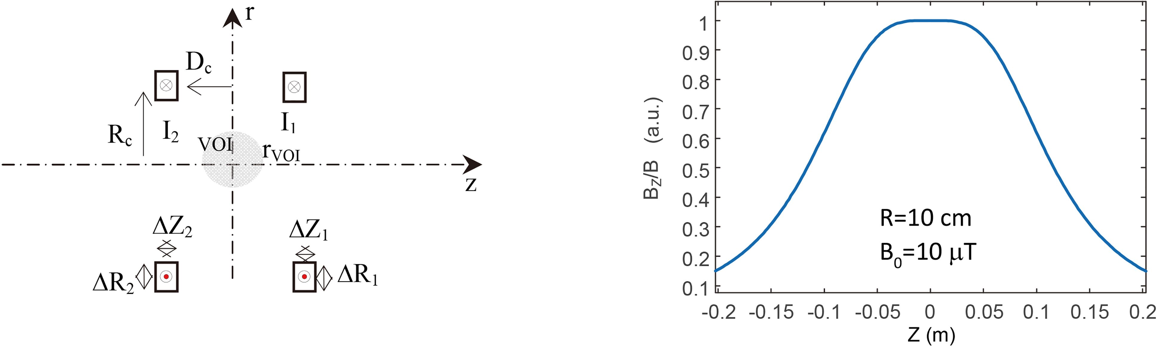
The DPF
In order to show the Paretian nature of the RD problem, we report in Fig. 2 the Pareto front obtained for a stochastic approach based on Eq. (1). To estimate mean and variance at each trial solution, a MC analysis with 300 cases has been run. Tolerance
Pareto front for a stochastic approach.
Pareto front for a worst-case approach.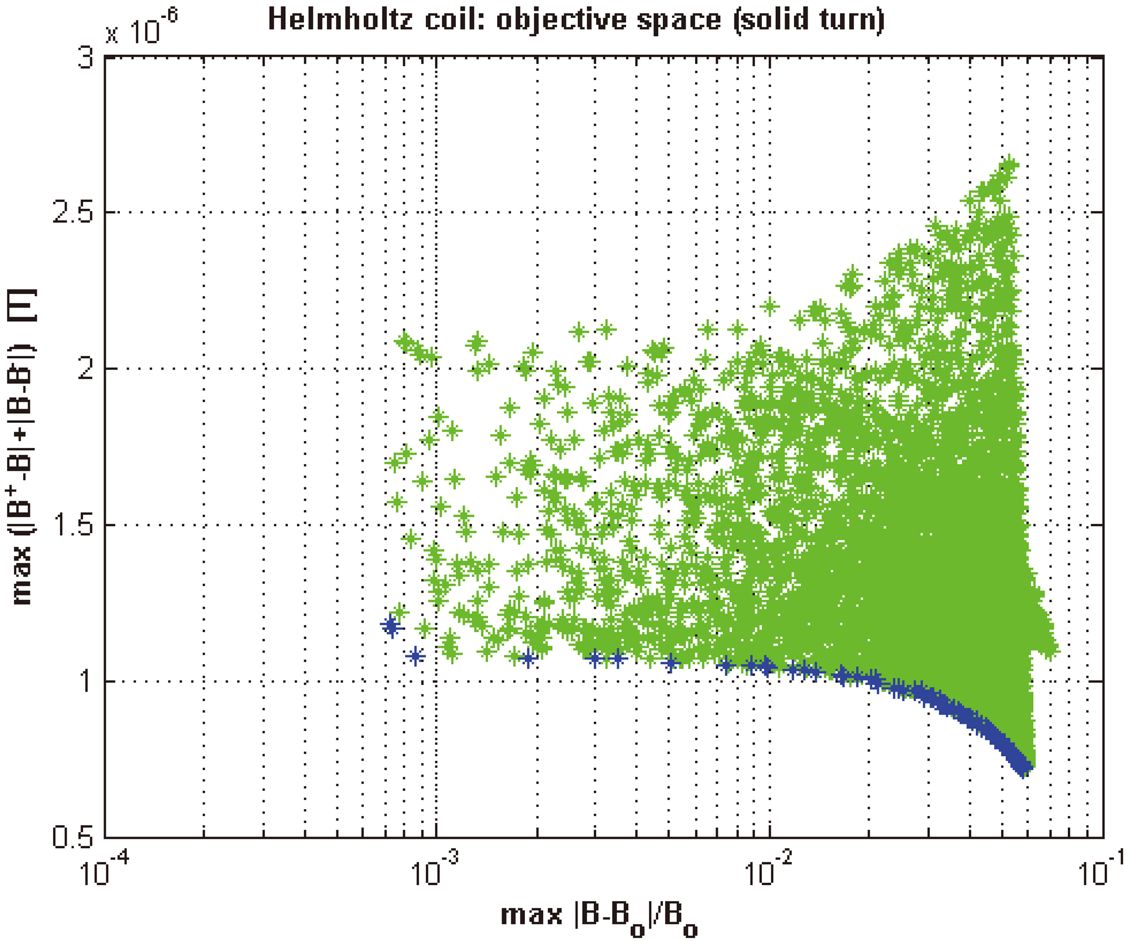
Results of TA on
It is interesting to note that the solution located at the left end of the Pareto front in Fig. 3 (minimal field homogeneity) corresponds just to the Helmholtz’s classical solution for
Note that the symmetry of design is lost when the effect of tolerances is considered, and parameters must be considered each different from the others. A TA was also performed for this test example to assess performance reduction due to this effect: tolerances on all parameters have been assumed uncorrelated and normally distributed, with a standard deviation equal to 1.2% of the nominal value (corresponding to 99.9% of cases falling inside the tolerance range), except for the radius, for which a tolerance of 50
CFSO optimization results
CFSO configuration and computational time
Solutions in the objective space for both approaches (LHS 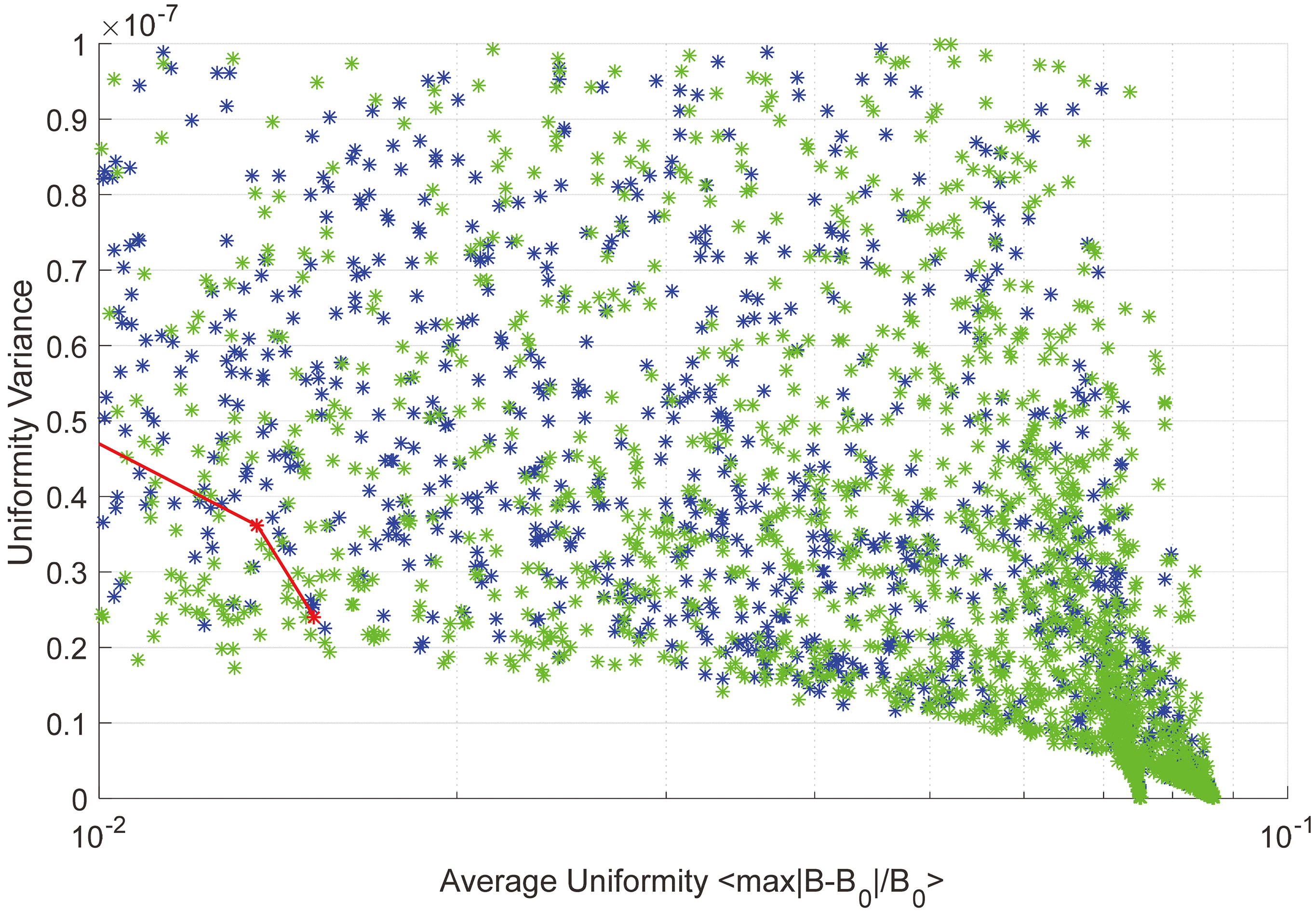
To assess the impact of “robust” formulation on the optimization of electromagnetic device, the CFSO algorithm was used to find the best robust configuration of the coils. Radius and mutual distance of the coils are both considered DOF, independent each to the other, while coils thickness, length and current are considered UP. For each trial solution, a stochastic tolerance analysis is performed, and the objective function is a linear combination of average and standard deviation of field uniformity. Different weights have been tried for the linear combination but best results have been obtained by 1:1 ratio (i.e. direct sum). The optimization of the cost function was performed using two techniques: an exhaustive LHS paired with a Levenberg-Marquardt local search algorithm (LM) to trace the boundaries of the objective space, and a swarm based global optimization technique based on the CFSO algorithm. Results are shown in Fig. 4. The best numerical solution found by the CFSO is reported in Table 2, along with the configuration parameters and the computational costs associated to the cost function in Table 3. Computational times are relative to an Intel Processor Core i7 @2.40 GHz.
Robust design and tolerance analysis are more and more emerging as lively research field in the area of optimization in electromagnetism. Different approaches are possible to cope with this problem. In this paper, with the aim to present different, possible ways to formulate robust design algorithms, two methods have been presented, showing their Paretian nature. The additional computational efforts required by robust formulations call for tools able to reduce computation times: a few of them have been presented in the paper, together with an original, highly effective optimization algorithm based on a continuous formulation of flock of starlings, providing control of trajectories in DOF space through control of poles of a continuous system. A simple illustrative example has been used to show practically the different aspects of the robust design problem and of the tools discussed in the paper.
Footnotes
Acknowledgments
This paper was a joint work among different research groups in the Italian community of Optimization and Inverse Problems in Electromagnetism. Authors wish to thank all the researchers in the community, and particularly Dr. Lozito, from Univ. Roma Tre, Dr. Chiariello, from Univ. della Campania “Luigi Vanvitelli” for their contribution to the work.