Radial basis function and finite element method hybrid approach for three-dimensional electromagnetics problems

Abstract

This paper presents a Radial Basis Function (RBF) and Finite Element Method (FEM) hybrid approach to solve a 3-D electromagnetic problem. The proposed method divides the entire computational domain into a series of sub-domains. The shape functions of each sub-domain are obtained by point interpolation method based on RBF to improve fitting performance of FEM. Each sub-domain consists of Galerkin FEM elements in the entire computational domain. To validate the proposed method, a case study is carried out based on a dual-electrode DC arc furnace. The results demonstrate that RBF and FEM hybrid approach in this paper is superior to the traditional FEM.

Keywords

Finite element method radial basis function magnetic vector potential three dimensional (3-D)

1. Introduction

In recent years, many researchers have presented efforts for element free methods to decrease computational complexity of traditional FEM [1–4]. Element-free Galerkin (EFG) method is one of the most popular element free methods. However, the shape functions of EFG cannot satisfy Kronecker delta property, which is very important in FEM. Then, it does not vanish on boundaries where the Dirichlet boundary conditions are imposed [5]. To resolve the problem of EFG, RBF collocation method is presented in this paper, which has significant advantages in solving typical electromagnetic field problems [6,7]. The shape function based on RBF uses a nonlinear approximation, which is likely closer to the actual result than the FEM. In this case, Dirichlet boundary conditions can be directly imposed. As a kind of global basis function, the coefficient matrix of the RBF collocation method would be full and asymmetric, which restrict the application of this method for solving complex electromagnetic problems [8]. Meanwhile, it is difficult to handle the interface condition of two different homogeneous media [9,10].

Some researchers presented RBF and FEM hybrid approach (RBF-FEM) for solving 2-D electromagnetic field problems, and verified the efficiency of this hybrid method [11]. The entire coefficient matrix of RBF-FEM is sparse. In addition, RBF-FEM is easy to deal with the complex boundary conditions as FEM. These 2-D problems were only computed in [11], but no suggestions were provided for extending the solutions to 3-D problems. Compared with 2-D problems, a 3-D electromagnetic problem requires much more complex mesh, proper boundary conditions, nodes, and memory space. Meanwhile, the stability and convergence of RBF-FEM is not verified for solving the 3-D problems, which makes application of RBF-FEM in 3-D difficult and important.

This paper uses RBF-FEM to solve a 3-D electromagnetic field with a case study base on a dual-electrode DC arc furnace. The entire computational domain is divided into a series of sub-domains, and the shape functions are obtained by an interpolation method based on RBF. Each sub-domain consists of elements of Galerkin FEM to solve the electromagnetic field of the entire computational domain.

In the next section we describe the formulation of RBF-FEM. A numerical example is presented in Section 3. Finally, Section 4 contains conclusions.

2. Implementation of the RBF-FEM Method for 3-D electromagnetic field

In order to formulate the hybrid method in this paper, the entire computational domain is divided into a series of sub-domains, and each sub-domain is considered as the elements of Galerkin FEM.

The governing equations in each sub-domain 𝛺_i can be simply written as [12]: $\begin{eqnarray}\displaystyle \left\{\begin{array}{@{}l@{}}La_{i}=f∼\text{in}∼{\Omega}_{i}\\ Ba_{i}=g∼\text{on}∼\partial {\Omega}_{i}\end{array}\right. & & \displaystyle\end{eqnarray}$ (1) where L is a linear differential operator, f is the applied source or forcing function, and a _i is the unknown quantity.

The entire computational domain is shown in Fig. 1.

Fig. 1.

Entire computational domain.

2.1. Shape function constructed by RBF

In sub-domain 𝛺_i with N _i collocation nodes set, the approximate solution A _i can be expressed as [11]: $\begin{eqnarray}\displaystyle A_{i}=\mathop{\sum }_{j=1}^{N_{i}}b_{j}Q_{j}(\mathbf{x})=\mathbf{Q}_{i}^{T}(\mathbf{x})\mathbf{b}_{i} & & \displaystyle\end{eqnarray}$ (2) where b _i is the unknown coefficient vector, and Q _i(x) is the RBF vector.

There are many kinds of RBFs, such as Gaussian function. This paper chooses multiquadrics (MQ) radial basis function for its superior performance [11]. In the 3-D Cartesian coordinate system, the MQ-RBF is expressed as $\begin{eqnarray}\displaystyle Q_{j}(\mathbf{x})=Q_{j}(x,y,z)=\sqrt{(x-x_{j})^{2}+(y-y_{j})^{2}+(z-z_{j})^{2}+p_{j}^{2}} & & \displaystyle \nonumber\end{eqnarray}$ where p _j is a shape parameter that influences the fitting accuracy, and the (x _j, y _j, z _j) are the coordinates of interpolation points.

According to Eq. (2), the value of each collocation point in computational domain 𝛺_i can be written as the following form. $\begin{eqnarray}\displaystyle \left[\begin{array}{@{}c@{}}A(\mathbf{x}_{1})_{i}\\[2.0pt] \vdots \\[2.0pt] A(\mathbf{x}_{j})_{i}\\[2.0pt] \vdots \\[2.0pt] A(\mathbf{x}_{N_{i}})_{i}\end{array}\right]=\left[\begin{array}{@{}c@{}}Q_{1}(\mathbf{x}_{1})\ldots Q_{j}(\mathbf{x}_{1})\ldots Q_{N_{i}}(\mathbf{x}_{1})\\[2.0pt] \vdots \\[2.0pt] Q_{1}(\mathbf{x}_{j})\ldots Q_{j}(\mathbf{x}_{j})\ldots Q_{N_{i}}(\mathbf{x}_{j})\\[2.0pt] \vdots \\[2.0pt] Q_{1}(\mathbf{x}_{N_{i}})\ldots Q_{j}(\mathbf{x}_{N_{i}})\ldots Q_{N_{i}}(\mathbf{x}_{N_{i}})\end{array}\right]\mathbf{b}_{i}. & & \displaystyle\end{eqnarray}$ (3) To simplify Eq. (3), let $\begin{eqnarray}\displaystyle \mathbf{a}_{i}=\left[A(\mathbf{x}_{1})_{i}\ldots A(\mathbf{x}_{N_{i}})_{i}\right]^{T} & & \displaystyle \nonumber\\ \displaystyle \mathbf{B}=\left[Q_{i}(\mathbf{x}_{1})\ldots Q_{i}(\mathbf{x}_{N_{i}})\right]^{T}. & & \displaystyle \nonumber\end{eqnarray}$ The solution A _i is $\begin{eqnarray}\displaystyle \mathbf{A}_{i} & = & \displaystyle \mathbf{Q}_{i}^{T}(\mathbf{x})\mathbf{b}_{i}=\mathbf{Q}_{i}^{T}(\mathbf{x})\mathbf{B}^{-1}\mathbf{a}_{i}\nonumber\\ \displaystyle & = & \displaystyle {\varphi}_{i}a_{ix}\mathbf{e}_{x}+{\varphi}_{i}a_{iy}\mathbf{e}_{y}+{\varphi}_{i}a_{iz}\mathbf{e}_{z}=\boldsymbol{{\varphi}}_{im}\mathbf{a}_{i},\quad m=x,y,z\nonumber\end{eqnarray}$ where a _ix, a _iy and a _iz are the three components of the A _i in the direction of x, y and z.

𝜑 _im is expressed as $\begin{eqnarray}\displaystyle \boldsymbol{{\varphi}}_{im}=\left\{\begin{array}{@{}l@{}}{\varphi}_{i}\mathbf{e}_{x},\quad m=x\\ {\varphi}_{i}\mathbf{e}_{y},\quad m=y\\ {\varphi}_{i}\mathbf{e}_{z},\quad m=z\end{array}\right.. & & \displaystyle \nonumber\end{eqnarray}$ The vector form of shape function 𝜑 _i can be expressed as $\begin{eqnarray}\displaystyle \boldsymbol{{\varphi}}_{i}=\mathbf{Q}_{i}^{T}(\mathbf{x})\mathbf{B}^{-1}. & & \displaystyle\end{eqnarray}$ (4)

2.2. Improved Galerkin FEM

After establishing the shape function by RBF, the entire computational domain is divided into several sub-domains. It transforms the governing equation of the electromagnetic field problem into weak integral form in the Galerkin’s weighted residual model, which reduce the complexity of computation dramatically. The rest of calculation process is the same as ordinary Galerkin FEM, but the shape function of the proposed hybrid method is constructed by RBF. The details of sub-domain dividing and node setting will be illustrated in the following numerical example.

3. Numerical example

To verify the efficiency of the RBF-FEM, the magnetic vector potential formulation is used to solve a 3-D static magnetic problem of a dual-electrode DC arc furnace. The dual-electrode DC arc furnace is used to smelt magnesium oxide. The schematic diagram of the dual-electrode DC arc furnace is shown in Fig. 2 [13]. The current flows through two electrodes (graphite anode and graphite cathode) with 10 kA. The magnesium oxide melts into a bath. Meanwhile, the thermal plasma arc is generated in the bottom of graphite anode and graphite cathode.

Fig. 2.

Schematic diagram of dual-electrode DC arc furnace.

The operating current of the dual-electrode DC arc furnace is direct current, so the field is a static magnetic field. The governing equation can be written as a vector Poisson’s equation. $\begin{eqnarray}\displaystyle {\nabla}^{2}\mathbf{A}=-{\mu}_{0}\mathbf{J} & & \displaystyle\end{eqnarray}$ (5) where A is the magnetic vector potential, 𝜇₀ is the vacuum permeability, and J is the current density.

According to [14], the model of the bath can be assumed to be an elliptic cylinder. In this paper, the dimensions of the dual-electrode DC arc furnace and bath are shown in Table 1 and Fig. 3.

Table 1

Dimensions of the furnace.

The furnace height (m)	The furnace diameter (m)	Electrode diameter (m)	The distance between electrodes center (m)
2.00	2.00	0.35	0.75

Fig. 3.

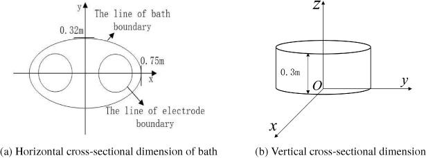
Bath cross-sectional dimension.

In Fig. 3, the bath is axially symmetric about the Z axis. So we only investigate a 1/2 section of the bath.

The boundary conditions of the bath domain are shown in Fig. 4.

Fig. 4.

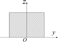
Boundary conditions of the bath domain.

The symmetrical boundary conditions of the bath domain (Fig. 4) are written as $\begin{eqnarray}\displaystyle \left\{\begin{array}{@{}l@{}}A_{y}=0,\quad \text{on }S_{1}\\[3.0pt] \displaystyle \frac{\partial A_{x}}{\partial x}=0,\quad \text{on }S_{1}\\[4.0pt] A_{z}=0,\quad \text{on }S_{1}\end{array}\right. & & \displaystyle\end{eqnarray}$ (6) where S ₁ is the surface of the yOz.

Far field boundary conditions are shown in Fig. 5.

Fig. 5.

Far field boundary conditions.

Far field boundary conditions are written as $\begin{eqnarray}\displaystyle S_{r}:A_{x}=A_{y}=A_{z}=0 & & \displaystyle\end{eqnarray}$ (7) In the 3-D Cartesian coordinate system, the weak integral form of Eq. (5) is $\begin{eqnarray}\displaystyle \left\{\begin{array}{@{}l@{}}\displaystyle \int _{{\Omega}}{\nabla}\boldsymbol{{\varphi}}_{i}\cdot {\nabla}\mathbf{A}dV-\displaystyle \int _{{\Omega}}{\mu}_{0}\boldsymbol{{\varphi}}_{i}\cdot \mathbf{J}dV=0\\[3.0pt] A_{y}=0,\quad \text{on }S_{1}\\[3.0pt] A_{z}=0,\quad \text{on }S_{1}\\[3.0pt] A_{x}=A_{y}=A_{z}=0,\quad \text{on }S_{r}\end{array}\right. & & \displaystyle\end{eqnarray}$ (8) where 𝜑 _i is the vector form of shape function, 𝛺 is the entire computational domain.

By Eq. (4), the Eq. (8) can be expressed as $\begin{eqnarray}\displaystyle \int _{{\Omega}}[{\nabla}(\mathbf{Q}_{i}(\mathbf{x})^{T}\mathbf{B}^{-1})]^{T}\cdot [{\nabla}(\mathbf{Q}_{i}(\mathbf{x})^{T}\mathbf{B}^{-1})]dV\mathbf{a}_{\mathbf{i}}-\int _{{\Omega}}{\mu}_{0}(\boldsymbol{Q}_{i}(\mathbf{x})^{T}\mathbf{B}^{-1})\cdot \mathbf{J}dV=0 & & \displaystyle \nonumber\end{eqnarray}$ Then, we get $\begin{eqnarray}\displaystyle \int _{{\Omega}}[{\nabla}(\mathbf{Q}_{i}(\mathbf{x})^{T}\mathbf{B}^{-1})]^{T}\cdot [{\nabla}(\mathbf{Q}_{i}(\mathbf{x})^{T}\mathbf{B}^{-1})]dV\mathbf{a}_{\mathbf{i}}=\int _{{\Omega}}{\mu}_{0}(\mathbf{Q}_{i}(\mathbf{x})^{T}\mathbf{B}^{-1})\cdot \mathbf{J}dV & & \displaystyle \nonumber\end{eqnarray}$ Constructing the linear system of equations $\begin{eqnarray}\displaystyle \mathbf{Da}_{i}=\mathbf{C} & & \displaystyle \nonumber\end{eqnarray}$ where D = ∫_𝛺[𝛻(Q _i(x)^T B ⁻¹)]^T ⋅ [𝛻(Q _i(x)^T B ⁻¹)]dV is the coefficient matrix, a _i is the solution vector, and C = 𝜇₀∫_𝛺(Q _i(x)^T B ⁻¹) ⋅J dV = 𝜇₀[∫_𝛺(𝜑_i1 J)dV …∫ _𝛺(𝜑_{iN
_i} J)dV ]^T.

The shape functions of the RBF-FEM satisfy the Kronecker delta property [15], hence the integral of RBF-FEM is restricted to every belonging sub-domain. Moreover, the integral of the shape function in the interface of two adjacent sub-domains is calculated.

First, the current density of the dual-electrode DC arc furnace is calculated by FEM (ANSYS software), which is shown in Fig. 6. Then Fig. 7 shows the current density distribution on the bottom of the cathode. Second, in accordance with the current density distribution on the bottom of the cathode, the entire computational domain is divided into twenty sub-domains. Figure 8 shows the domain decomposition diagram of RBF-FEM, each sub-domain is marked as different serial numbers and letters. In particular, the domain 5 is divided into eight small sub-domains by polygonal approximation method. The 11 × 11 × 11 interpolation nodes of the sub-domains (serial number 1–4) are set. The 11 × 5 × 11 interpolation nodes in each small sub-domains of serial number 5 are set. The sub-domains of serial number t (t ₁), u (u ₁), v (v ₁) and w (w ₁) are very small, and the 5 × 3 × 11 interpolation nodes are set. In order to obtain the accurate results, the interpolation nodes of the sub-domains obey uniform distribution.

Fig. 6.

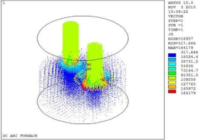
Current density distribution of the dual-electrode DC arc furnace (A∕m²).

Fig. 7.

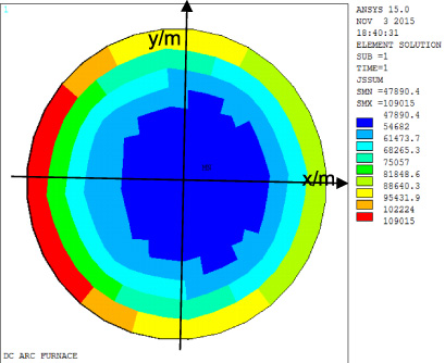
Current density distribution on the bottom of the cathode (A∕m²).

Fig. 8.

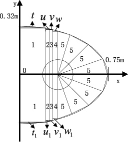
Sub-domain distribution of RBF-FEM.

The magnetic vector potential formulation of the bath is solved by RBF-FEM, which p is 0.0162. The contour plots of magnetic vector potential for the bath are shown in Fig. 9–Fig. 13 (Because the entire computational domain is axially symmetric about X-axis, the contour plots of magnetic vector potential in the sub-domains of serial number t, u, v and w are only shown.).

Fig. 9.

Contour plots of magnetic vector potential (the domain 1 and t (T ⋅ m)).

Fig. 10.

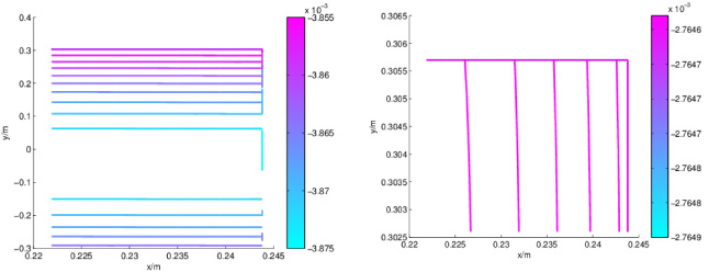
Contour plots of magnetic vector potential (the domain 2 and u (T ⋅ m)).

Fig. 11.

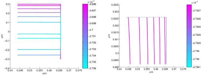
Contour plots of magnetic vector potential (the domain 3 and v (T ⋅ m)).

Fig. 12.

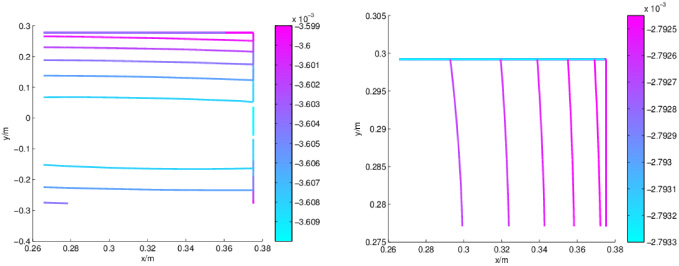
Contour plots of magnetic vector potential (the domain 4 and w (T ⋅ m)).

Fig. 13.

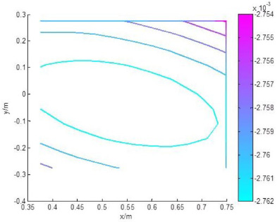
Contour plots of magnetic vector potential (the domain 5 (T ⋅ m)).

To demonstrate the accuracy of the result, the magnetic vector potential equation of the bath is solved by FEM (Reduced Standard Potential (RSP)). Taking the horizontal cross-section (z = 0.3 m) of the bath, the numerical results of FEM are shown in Fig. 14.

Fig. 14.

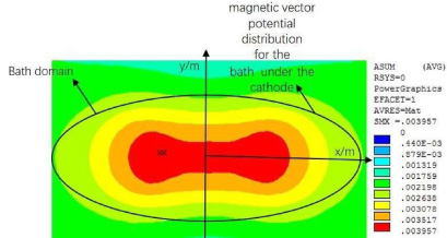
Contour plots of the magnetic vector potential for the bath (z = 0.3 m, T ⋅ m).

Meanwhile, we define the error as $\begin{eqnarray}\displaystyle \text{error}=|A_{R}-A_{F}| & & \displaystyle \nonumber\end{eqnarray}$ where A _R is the result by implementing RBF-FEM, and A _F is the result by FEM.

The numerical results (x = 0 m, z = 0.3 m) of RBF-FEM and FEM are compared, as shown in Fig. 15.

Fig. 15.

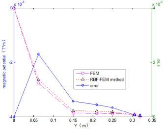
Solutions of magnetic vector potential using the RBF-FEM method compared with the FEM along the line x = 0 m, z = 0.3 m.

In accordance with the flow of current within the bath, the downward direction of magnetic vector potential is positive direction. Figure 9–Fig. 13 appear the negative values, and they indicate that the direction of the magnetic vector potential is opposite to positive direction.

The number 2 and number 3 sub-domains are very small, so the magnetic vector potential presents linear distribution. The sub-domains with serial number t, u, v and w appear the magnetic vector potential distributions whose directions are all approximately the X-axis direction. However, it can be seen that (the sub-domains of serial number t, u, v and w) the values of the magnetic vector potential almost are equal. The same scale in the contour plots are represented with the same colors by FEM [16]. Meanwhile, the contour plots of four small sub-domains (the sub-domains of serial number t, u, v and w) can be represented with the same color. The results of RBF-FEM (Fig. 9–Fig. 13) and FEM (Fig. 14) are compared at the Y-axis of the bath (z = 0.3 m). Figure 15 shows that the results of RBF-FEM agree well with the calculations of FEM.

To prove the efficiency of RBF-FEM, Intel Visual FORTRAN 2011 is used to implement the code and all computations were carried out on a Windows 8 system with Intel-core i5 CPU and 8.00 GB RAM. The computational cost and CPU time comparison (numerical example) between FEM and RBF-FEM is shown in Table 2.

Table 2

Computational cost and CPU time comparison between FEM and RBF-FEM

Method	FEM	RBF-FEM
Elements (Sub-domains)	14219	20
Nodes	16225	11484
CPU Time (s)	80.134	63.065
Memory Space (MB)	177.651	83.267

Considering the validation results, the RBF-FEM is extended to solving the 3-D electromagnetic problem. In case of 3-D problem, the solution process requires high memory and is the most consuming time. From the results of Table 2, RBF-FEM is easier meshing than traditional FEM. Because the shape function constructed by RBF is non-linear approximation and will be closer to the actual solution of sub-domain. Further, as the RBF shows improving convergence performance, the RBF-FEM requires less node.

4. Conclusion

In this paper, the RBF-FEM hybrid method has been implemented in the 3-D electromagnetic problem. To illustrate the efficiency of RBF-FEM, the magnetic vector potential formulation is used to solve a 3-D static problem of a dual-electrode DC arc furnace. By analyzing the validation results, RBF-FEM requires less meshing, fewer nodes, and lower computational complexity compared with traditional FEM. In addition, the sub-domains of RBF-FEM are considered as elements of Galerkin FEM, so it is easy to handle the interface condition of two different homogeneous medium as FEM. In the future work, one may consider solving three dimensional electromagnetic field problems by RBF-FEM.

Footnotes

Acknowledgements

This work was supported by National Natural Science Foundation of China (Grant No. 51604059), and the Fundamental Research Funds for the Central Universities (Grant No. DUT16QY35, and No. 2342017DUT17RC (4)04).

References

Zhang

Shao

K.R.

and Guo

, Multiquadrics collocation method for transient eddy current problems, IEEE Transactions on Magnetics 42 (2006), 3183–3185, doi:10.1109/TMAG.2006.8800-88.

Chen

Zhang

and Ding

, Field analysis of a sinusoidal-edged Halbach magnet array using the differential quadrature finite element method, International Journal of Applied Electromagnetics and Mechanics 50 (2016), 63–80, doi:10.3233/JAE-150069.

Kawaguchi

Satoh

and Timoshkin

I.V.

, Boundary element analysis of stress forces in pulsed electric field treatment of microorganism, International Journal of Applied Electromagnetics and Mechanics 53 (2017), 315–325, doi:10.3233/JAE-160047.

Liu

Xie

Pei

and Chen

, Numerical simulation method for IR thermography NDE of delamination defect in multilayered plate, International Journal of Applied Electromagnetics and Mechanics 52 (2016), 381–389, doi:10.3233/JAE-162121.

Parreira

G.F.

Silva

E.J.

and Fonseca

A.R.

, The element-free Galerkin method in three-dimensional electromagnetic problems, IEEE Transactions on Magnetics 42 (2006), 711–714, doi:10.1109/TMAG.2006.872014.

Viana

S.A.

Rodger

and Lai

H.C.

, Application of the local radial point interpolation method to solve eddy current problems, IEEE Transactions on Magnetics 42 (2006), 591–594, doi:10.1109/TMAG.2006.871966.

Lai

S.J.

Wang

B.Z.

and Duan

, Meshless radial basis function method for transient electromagnetic computations, IEEE Transactions on Magnetics 44 (2008), 2288–2295, doi:10.1109/TMAG.2008.2001796.

Yang

Chen

and Lei

, Domain decomposition combined radial basis function collocation method to solve transient eddy current magnetic problems with moving conductors, IEEE Transactions on Magnetics 47 (2011), 2939–2942, doi:10.1109/TMAG.2011.2146240.

S.L.

Yang

Wong

H.C.

and Ni

, A meshless collocation method based on radial basis functions and wavelets, IEEE Transactions on Magnetics 40 (2004), 1021–1024, doi:10.1109/TMAG.2004.824778.

10.

Chen

Lei

and Yang

, Using improved domain decomposition method and radial basis functions to determine electromagnetic fields near material interfaces, IEEE Transactions on Magnetics 48 (2012), 199–202, doi:10.1109/TMAG.2011.2173750.

11.

Zou

Lei

and Shao

K.R.

, Hybrid approach of radial basis function and finite element method for electromagnetic problems, IEEE Transactions on Magnetics 51 (2015), 1–4, doi:10.1109/TMAG.2014.2354371.

12.

Jin

, The Finite Element Method in Electromagnetics, Wiley, New York, America, 1993.

13.

Reynolds

Q.G.

, The dual-electrode DC arc furnace-modelling insights, Journal of the Southern African Institute of Mining and Metallurgy 111 (2011), 697–704.

14.

Wang

N.H.

and Li

, Computational analysis of a twin-electrode DC submerged arc furnace for MgO crystal production, Journal of Materials Processing Technology 211 (2011), 388–395.

15.

Zhang

and Liu

, Meshless Method, Tsinghua University Press, Beijing, China, 2009.

16.

Ling

L.G.

, ANSYS14.0 Thermodynamic Analysis from Entry to the Master, Tsinghua University Press, China, 2013, pp. 102–110.