A novel eight-pole heteropolar radial-axial hybrid magnetic bearing

Abstract

This paper proposes a novel eight-pole heteropolar radial-axial hybrid magnetic bearing (HMB) to reduce the power consumption and to improve the space utilization of the entire system. The mathematical model of HMB is obtained by applying the equivalent magnetic circuit method. And its bearing capacity in both the radial and axial directions is analyzed. Also, to maximize the bearing capacity, the structural parameters of HMB are designed. The magnetic field distribution and the magnetic induction intensity across the air gap are studied by the 3D Finite Element (FE) simulation. And the force/current and force/displacement characteristics are then attained. Experiments on the investigated HMB are carried out to validate the modelling results. It has been shown that the maximum bearing capacity of the HMB is 190 N and 170 N in the radial and axial directions respectively, which are the 82.6% and 81% of theoretical value.

Keywords

Hybrid magnetic bearing permanent-magnet-biased bearings capacity equivalent magnetic circuit combined radial-axial structure

1. Introduction

Magnetic bearings possess many advantages over traditional mechanical bearings, such as contactless, free of lubrication, high operational speed, and adjustable stiffness damping [1–5]. In recent decades, a new type of magnetic bearings, i.e. hybrid magnetic bearings (HMB), has been developed and been increasingly utilized in various industrial sectors, such as in aerospace applications, the energy storage flywheel systems, the wind power generation, artificial heart blood pumps, and the high blower and compressor [6–11], due to their reduced power consumption, smaller the coil number of electromagnet turns, the compact system configuration, as well as the increased bearing capability. Figure 1(a) schematically shows the configuration of a typical HMB, which consists of the stator, the rotor, permanent magnets, control coils, displacement sensors, the controller, and the power amplifier. The HMBs can be categorized into the axial HMB, the radial HMB, and the combined radial-axial HMB [12] according to their functions. Based on the polarity of the bias magnetic field, they can be characterized as the heteropolar and the homopolar HMB [13]. In the heteropolar configuration, the local magnetic flux density on the rotating shaft can vary between +B ₀ and −B ₀ during one cycle, whereas the induction range of the homopolar bearing is always between 0 and +B ₀. There are many structures among the homopolar HMB. And the most common one is shown in Fig. 1(b) [14]. The Bias flux generated by the ring-shaped permanent magnet is depicted by the solid line. And the control flux generated by the control winding is shown by the dashed line. The main advantages of homopolar HMBs over heteropolar HMBs in general are lower eddy-current losses and less degradation of the load capacity with speed due to the eddy-currents induced in the rotor, so that they have been widely used in the industry. However, such magnetic bearings will have increased axial length to create a closed loop for bias flux, which in turn restricts the improvement of the critical speed of the rotor system. Moreover, the existing flux leakage coefficient of an axial crossing of this type of HMB is much larger than traditional eight-pole active magnetic bearings (AMBs) [15].

Fig. 1.

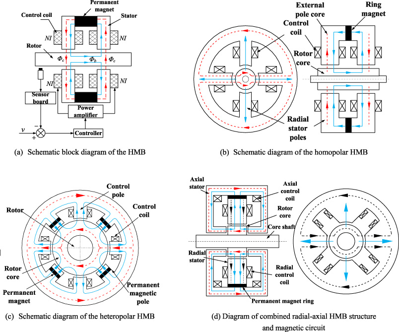
Schematic diagram of HMB.

Figure 1(c) shows the structure of a typical heteropolar HMB [16], where the bias magnetic circuit is indicated by the solid line and the control magnetic circuit is marked by the dashed line. The structure of the heteropolar HMB is similar to that of the AMB, but it can significantly reduce the magnetic flux leakage and the power loss compared to the AMB. Also, for a given load capacity, the axial dimension of this magnetic bearing is probably longer than that of most magnetic bearing. The length of the rotor affects rotordynamic margins and machine performance [17,18].

Yohji Okada proposed a kind of eight-pole heteropolar radial HMB [16,19], which has been subsequently studied by many researchers [20–23]. Compared to other heteropolar HMBs, the proposed one has simple mechanical construction and is relatively easy to control. Silicon steel sheets are used to fabricate the radial stators, leading to significantly reduction of the hysteresis and eddy current loss. The four radially controlled magnetic poles are separated by 90 degrees and the windings on the opposite poles are connected in series to produce a control flux (shown by the dashed line in Fig. 1(c)). The four radial permanent magnet poles that 45 degrees apart from the control poles are embedded with permanent magnets. The sheet permanent magnets produce biased magnetic fluxes (shown in solid lines in Fig. 1(c)). Lee established the mathematical model of the same polarity and heteropolar permanent magnetically biased magnetic bearing. And he also deduced the performance index formula of the same polarity permanent magnet offset magnetic bearing [24,25].

The combined radial-axial HMBs characterized in compact structure, small volume, short system length. And normally they have more complicated structure compared with radial HMBs and so on. Figure 1(d) shows a classical configuration of such HMB with a compact structure and high space utilization, Hawkins.L applied this technique for the suspension of the five-degree-of-freedom energy storage flywheel [26]. McMullen [27] also incorporated such structure into the energy storage flywheel for uninterruptible power supply and power conditioning applications. Huang et al. [28] analyzed the distribution of the magnetic flux leakage path and the air gap flux in this structure to deduce its accurate mathematical model. Mei et al. [29] proposed a parameter design method of this structure based on magnetic flux calculation. Palazzolo’s team [30,31] and Calnetix [32] have recently developed a radial-axial homopolar MB for flywheel application.

In this paper, a novel eight-pole heteropolar radial-axial hybrid magnetic bearing was proposed. The section of radial magnetic bearing in integrated radial-axial integrated structure (proposed by McMullen) is replaced by eight-pole polarized permanent magnet bias radial magnetic bearing (originally proposed by Okada Y). Such new design combines the advantages of these two structures and optimizes the configuration of the axial stator so that it can offer simpler configuration, easier control method, and relatively small magnetic leakage as well as smaller axial size.

The remainder of this paper is organized as follows. Section 2 describes the structure of the proposed eight-pole heteropolar radial-axial HMB. The equivalent magnetic circuit analysis and mathematical model of the novel HMB are then demonstrated in Section 3. Section 4 presents its partial parameter design and Section 5 presents the simulation results of such HMB. Experiments are carried out in Section 6 to validate the modelling results. Conclusions are drawn in Section 7.

2. Structure and working principle

2.1. Structure

The basic structure with the magnetic circuit of the eight-pole heteropolar radial-axial HMB are schematically shown in Fig. 2. The radial stator consists of eight magnetic poles that are equispaced around its circumference. And the radial control coils are wound around the four control poles. Coils 1 and 2 are connected in series to produce a control flux in the vertical direction, while coils 3 and 4 are connected in series to produce a horizontal control flux. The four sheet-like permanent magnets are embedded in the permanent magnetic poles and located between the control poles for generating radial and axial biasing fluxes. The axial stator is wound around the control coil. And the coils 5 and 6 are connected in series to produce axial control flux. The opposed coils are connected in series. Both the radial stator and the rotor core are made of silicon steel sheets to reduce hysteresis effects and eddy current losses. The axial stator and silicon steel plate are made of electrician pure iron, which can reduce the coupling effect between the radial direction and the axial direction in such structure.

Fig. 2.

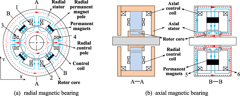
Diagram of the eight-pole heteropolar radial-axial HMB structure and magnetic circuit.

2.2. Working principle

As can be seen from Fig. 2, the bias magnetic flux (shown by the solid line, generated by the sheet-like permanent magnet) is divided into two parts upon passing through the permanent magnetic pole: one part passes through the rotor core, the radial air gap, and the radial control pole to form the closed loop, while the other part goes through the rotor core, axial air gap, and axial stator to contribute to another closed loop. The radial control coils 3, 4 produce the closed loop of the radial horizontal control flux that goes through the radial control of the magnetic pole, radial air gap, and the rotor core (shown by dotted line in Fig. 2(a)). The series connected axial control coils 5, 6 generate the closed loop of the axial control flux that travels through the axial stator, axial air gap, and the rotor core plate (shown by the dashed line in Fig. 2(b)). The net force is obtained by changing the net magnetic field, which is the sum of the permanent magnet field and the field generated by the coils. This could be achieved only by changing the current direction to modify the net generated field and the resulting force direction.

As shown in Fig. 2(a), when the rotor core is located at the center of the magnetic bearing, the size of each air gap is constant and the bias flux in the air gap is also constant, so that the resultant force that acting on rotor is zero. For instance, the rotor moves to the right when the rotor is subjected to the rightward disturbance in the horizontal direction. The right air gap decreases (the bias flux increases) while the left air gap increases (the bias flux decreases). Thus the resultant force enables the rotor move further to the right. The control coils 3 and 4 with the rated current would produce the horizontal leftward control flux, which can cancel the bias flux in the right air gap and meanwhile enhance the bias flux in the left air gap. This will lead to a larger magnetic flux in the left air gap than that in the right air gap. So the rotor will gradually return to the equilibrium position due to the horizontally leftward suction. Likewise, the rotor can always be pulled back to the equilibrium position based on the demonstrated control approach, no matter what disturbance acts on the rotor. The implemented control flux strategy results cross coupling between the horizontal and the vertical direction, which affect the operation of this bearing in the radial direction.

The working principle of the HMB in the axial direction is also given. As shown in Fig. 2(b), if the rotor core moves to the right by an axially rightward disturbing force, the right air gap will decrease (the bias flux will increase) and the left air gap will increase (the bias flux will decrease). The resultant force acting on the rotor enables its further movement to the right. The control coils 5 and 6 with rated current thus generate an axially leftward control flux that can cancel the bias flux in the right air gap and enhance the bias flux in the left air gap. The rotor will then gradually return to the equilibrium position by the axially leftward suction force as the consequence of larger magnetic flux in the left air gap. Similarly, the control principle is also applicable to the case under the left disturbance force in the axial direction.

3. Equivalent magnetic circuit analysis

The HMB structure is designed to achieve the maximum bearing capacity, so the formula of bearing capacity is required to provide a guideline for its structural design The formulas of radial and axial bearing capacity are obtained based on the analysis of the bias flux and control flux in the air gap. In this section, the equivalent magnetic circuit method is used to analyze the eight-pole heteropolar radial-axial HMB.

3.1. Equivalent magnetic circuit

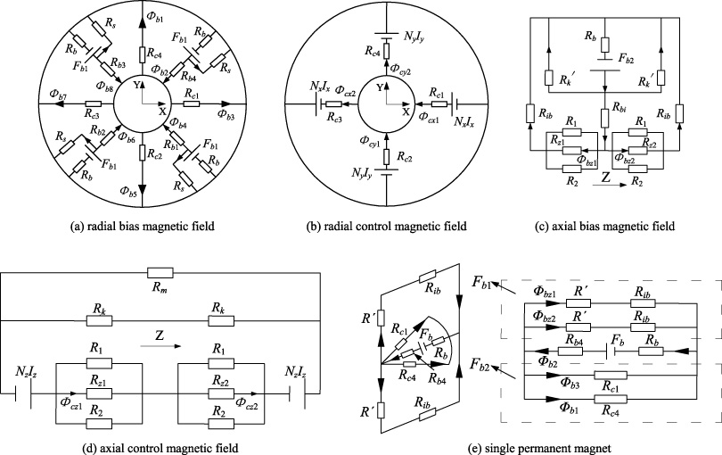
Considering the influence of magnetic flux leakage and soft magnetic reluctance, the exact equivalent magnetic circuits of both the radial and axial magnetic bearings was established, as illustrated in Fig. 3. Figure 3(a,b) shows the equivalent magnetic circuit of the radial magnetic bearing, where N _x I _x, N _y I _y denote the ampere-turns of radial control coil; R _c1 ∼ R _c4 are the air-gap reluctance of control pole; 𝜑_cxi, 𝜑_cyi are the control flux, F _b1 is the magnetomotive force of permanent magnet in the radial bias magnetic circuit equation; R _b1 ∼ R _b4 indicate the air gap reluctance of the permanent magnet magnetic pole; R _b, R _s represent the permanent magnet reluctance and reluctance of magnetic flux leakage respectively; and 𝜑_b1 ∼𝜑_b8 are bias flux. The magnetic permeability of Nd–Fe–B is close to that of the air (4π × 10 −7). The thickness of the permanent magnet (4 mm) is 8 times of the air gap (0.5 mm) of the magnetic bearing, so the reluctance of the permanent magnet is 8 times of that of the air gap correspondingly. And magnetic saturation is relatively serious near the lateral wall of permanent magnet. Therefore the control flux did not pass the pole of permanent magnet, the radial control flus circuit does not consider the PMs’ reluctance. The equivalent magnetic circuit of the axial magnetic bearing is demonstrated in Fig. 3(c,d). Hereby, N _z I _z is the ampere-turns of the axial control coils; R _z1, R _z2 are the axial air-gap reluctance; R _bi denotes the air-gap reluctance of the radial permanent magnet magnetic pole; R ₁, R ₂, R _k, R _{k
^′} are the reluctance of the magnetic flux leakage; R _m, R _ib are the reluctance of the iron core; F _b2 is the magnetomotive force of the permanent magnet in the axial bias magnetic circuit equation, 𝜑_cz1, 𝜑_cz2 are the control flux; and 𝜑_bz1, 𝜑_bz2 are the bias flux.

Fig. 3.

Equivalent magnetic circuit diagram.

3.2. Mathematical model

Due to the fact that the radial magnetic circuit is relatively short, in order to simplify the calculation, the reluctance of iron core is ignored, and the magnetic flux leakage coefficient of permanent magnet end face was taken as ϵ_b, with air gap magnetic flux leakage being ϵ. Thus, the effective magnetomotive force of permanent magnet can be calculated as F _b1∕ϵ_b. According to the magnetic circuit diagram and using Kirchhoff’s law, the radial control magnetic field equation can be obtained as $\begin{eqnarray}\displaystyle \left\{\begin{array}{@{}l@{}}{\phi}_{cx1}+{\phi}_{cy1}={\phi}_{cx2}+{\phi}_{cy2}\\ {\phi}_{cx1}R_{c1}-{\phi}_{cy1}R_{c2}=N_{x}I_{x}-N_{y}I_{y}\\ {\phi}_{cy1}R_{c2}-{\phi}_{cx2}R_{c3}=N_{x}I_{x}+N_{y}I_{y}\\ {\phi}_{cx2}R_{c3}-{\phi}_{cy2}R_{c4}=N_{x}I_{x}-N_{y}I_{y}.\end{array}\right. & & \displaystyle\end{eqnarray}$ (1)

Similarly, the radial bias magnetic field equation can be derived as $\begin{eqnarray}\displaystyle \left\{\begin{array}{@{}l@{}}{\phi}_{b2}(R_{b1}+R_{b})+{\phi}_{b3}R_{c1}=F_{b1}\\ {\phi}_{b4}(R_{b2}+R_{b})+{\phi}_{b3}R_{c1}=F_{b1}\\ {\phi}_{b4}(R_{b2}+R_{b})+{\phi}_{b5}R_{c2}=F_{b1}\\ {\phi}_{b6}(R_{b3}+R_{b})+{\phi}_{b5}R_{c2}=F_{b1}\\ {\phi}_{b6}(R_{b3}+R_{b})+{\phi}_{b7}R_{c3}=F_{b1}\\ {\phi}_{b8}(R_{b4}+R_{b})+{\phi}_{b7}R_{c3}=F_{b1}\\ {\phi}_{b8}(R_{b4}+R_{b})+{\phi}_{b1}R_{c4}=F_{b1}\\ {\phi}_{b2}+{\phi}_{b4}+{\phi}_{b6}+{\phi}_{b8}={\phi}_{b1}+{\phi}_{b3}+{\phi}_{b5}+{\phi}_{b7}.\end{array}\right. & & \displaystyle\end{eqnarray}$ (2)

By solving Eqs (1) and (2), the control flux and the bias flux at the radial air gap can be obtained in Eqs (3) and (4), respectively $\begin{eqnarray}\displaystyle \left\{\begin{array}{@{}l@{}}{\phi}_{cx1}=\displaystyle \frac{(1/R_{c2}+2/R_{c3}+1/R_{c4})N_{x}I_{x}+(-1/R_{c2}+1/R_{c4})N_{y}I_{y}}{1+R_{c1}/R_{c2}+R_{c1}/R_{c3}+R_{c1}/R_{c4}}\\[15.60004pt] {\phi}_{cy1}=\displaystyle \frac{(-1/R_{c1}+1/R_{c3})N_{x}I_{x}+(1/R_{c1}+1/R_{c3}+2/R_{c4})N_{y}I_{y}}{R_{c2}/R_{c1}+1+R_{c2}/R_{c3}+R_{c2}/R_{c4}}\\[15.60004pt] {\phi}_{cx2}=\displaystyle \frac{(2/R_{c2}+1/R_{c2}+1/R_{c4})N_{x}I_{x}+(-1/R_{c4}+1/R_{c2})N_{y}I_{y}}{R_{c3}/R_{c1}+R_{c3}/R_{c2}+1+R_{c3}/R_{c4}}\\[15.60004pt] {\phi}_{cy2}=\displaystyle \frac{(-1/R_{c3}+1/R_{c1})N_{x}I_{x}+(1/R_{c1}+2/R_{c2}+1/R_{c3})N_{y}I_{y}}{R_{c4}/R_{c1}+R_{c4}/R_{c2}+R_{c4}/R_{c3}+1}\end{array}\right. & & \displaystyle\end{eqnarray}$ (3) $\begin{eqnarray}\displaystyle \left\{\begin{array}{@{}l@{}}{\phi}_{b1}=\displaystyle \frac{F_{b1}R_{b}^{\prime }}{{\varepsilon}_{b}(R_{b}^{\prime }+R_{c}^{\prime })R_{c4}},\quad {\phi}_{b3}=\frac{F_{b1}R_{b}^{\prime }}{{\varepsilon}_{b}(R_{b}^{\prime }+R_{c}^{\prime })R_{c1}}\\[12.0pt] {\phi}_{b5}=\displaystyle \frac{F_{b1}R_{b}^{\prime }}{{\varepsilon}_{b}(R_{b}^{\prime }+R_{c}^{\prime })R_{c2}},\quad {\phi}_{b7}=\frac{F_{b1}R_{b}^{\prime }}{{\varepsilon}_{b}(R_{b}^{\prime }+R_{c}^{\prime })R_{c3}}\\[12.0pt] {\phi}_{b2}=\displaystyle \frac{F_{b1}R_{b}^{\prime }}{{\varepsilon}_{b}(R_{b}^{\prime }+R_{c}^{\prime })(R_{b1}+R_{b})},\quad {\phi}_{b4}=\frac{F_{b1}R_{b}^{\prime }}{{\varepsilon}_{b}(R_{b}^{\prime }+R_{c}^{\prime })(R_{b2}+R_{b})}\\[12.0pt] {\phi}_{b6}=\displaystyle \frac{F_{b1}R_{b}^{\prime }}{{\varepsilon}_{b}(R_{b}^{\prime }+R_{c}^{\prime })(R_{b3}+R_{b})},\quad {\phi}_{b8}=\frac{F_{b1}R_{b}^{\prime }}{{\varepsilon}_{b}(R_{b}^{\prime }+R_{c}^{\prime })(R_{b4}+R_{b})}.\end{array}\right. & & \displaystyle\end{eqnarray}$ (4)

In Eq. (4), the following relation is defined $\begin{eqnarray}\displaystyle \begin{array}{@{}l@{}}R_{b}^{\prime }=\displaystyle \frac{1}{R_{b1}+R_{b}}+\frac{1}{R_{b2}+R_{b}}+\displaystyle \frac{1}{R_{b3}+R_{b}}+\frac{1}{R_{b4}+R_{b}},\\[14.39996pt] R_{c}^{\prime }=\displaystyle \frac{1}{R_{c1}}+\frac{1}{R_{c2}}+\frac{1}{R_{c3}}+\frac{1}{R_{c4}}.\end{array} & & \displaystyle\end{eqnarray}$ (5)

Due to longer axial magnetic circuit, the effect of iron core reluctance on magnetic field has to be considered. The reluctance of the axial air gap can be calculated as $\begin{eqnarray}\displaystyle R^{\prime }=\frac{R_{1}R_{2}R_{z1}}{R_{1}R_{2}+R_{1}R_{z1}+R_{2}R_{z1}}={\varepsilon}\cdot R_{z1}={\varepsilon}\cdot R_{z2}. & & \displaystyle\end{eqnarray}$ (6) Therefore, the total reluctance of axial control magnetic circuit R ₀ is $\begin{eqnarray}\displaystyle R_{0}=\frac{2R_{k}R_{m}}{2R_{k}+R_{m}}+2R^{\prime }. & & \displaystyle\end{eqnarray}$ (7) Also, the total flux of the axial magnetic circuit can be given as $\begin{eqnarray}\displaystyle {\phi}_{0}=\frac{2N_{z}I_{z}}{R_{0}}. & & \displaystyle\end{eqnarray}$ (8) Furthermore, the control flux of the axial air gap can be obtained $\begin{eqnarray}\displaystyle \left\{\begin{array}{@{}l@{}}{\phi}_{cz1}=\displaystyle \frac{{\phi}_{0}\cdot {\varepsilon}R_{z1}}{R_{z1}}=\frac{2N_{z}I_{z}}{{\varepsilon}\cdot \left(\frac{2R_{k}R_{m}}{2R_{k}+R_{m}}+{\varepsilon}R_{z1}+{\varepsilon}R_{z2}\right)}\\[24.0pt] {\phi}_{cz2}=\displaystyle \frac{{\phi}_{0}\cdot {\varepsilon}R_{z2}}{R_{z2}}=\frac{2N_{z}I_{z}}{{\varepsilon}\cdot \left(\frac{2R_{k}R_{m}}{2R_{k}+R_{m}}+{\varepsilon}R_{z1}+{\varepsilon}R_{z2}\right)}.\end{array}\right. & & \displaystyle\end{eqnarray}$ (9)

Revisiting Fig. 3(b,c), the total bias flux of the axial magnetic circuit can be obtained $\begin{eqnarray}\displaystyle {\phi}=\frac{F_{b2}/{\varepsilon}}{(R^{\prime }+4R_{ib})/8+R_{b}+R_{bi}}=\frac{8F_{b2}}{{\varepsilon}(R^{\prime }+4R_{ib}+8R_{b}+8R_{bi})}. & & \displaystyle\end{eqnarray}$ (10)

And the axial bias flux can be calculated as $\begin{eqnarray}\displaystyle {\phi}_{bz1}={\phi}_{bz2}=\frac{{\phi}R^{\prime }}{8R_{z1}} & = & \displaystyle \frac{F_{b2}R^{\prime }}{{\varepsilon}(R^{\prime }+4R_{ib}+8R_{b}+8R_{bi})R_{z1}}\nonumber\\ \displaystyle & = & \displaystyle \frac{F_{b2}R^{\prime }}{{\varepsilon}(R^{\prime }+4R_{ib}+8R_{b}+8R_{bi})R_{z2}}\nonumber\\ \displaystyle & = & \displaystyle \frac{F_{b2}{\varepsilon}}{{\varepsilon}_{b}({\varepsilon}R_{z1}+4R_{ib}+8R_{b}+8R_{bi})}\nonumber\\ \displaystyle & = & \displaystyle \displaystyle \frac{F_{b2}{\varepsilon}}{{\varepsilon}_{b}({\varepsilon}R_{z2}+4R_{ib}+8R_{b}+8R_{bi})}.\end{eqnarray}$ (11)

Assume that the tiny displacements of the rotor in the X, Y and Z positive directions are x, y, z, respectively. We can derive the air-gap reluctance at the working air gap as $\begin{eqnarray}\displaystyle R_{c1}=\frac{g_{0}-x}{{\mu}_{0}S_{xy}},\quad R_{c3}=\frac{g_{0}+x}{{\mu}_{0}S_{xy}},\quad R_{c2}=\frac{g_{0}+y}{{\mu}_{0}S_{xy}},\quad R_{c4}=\frac{g_{0}-y}{{\mu}_{0}S_{xy}}. & & \displaystyle\end{eqnarray}$ (12)

The air-gap reluctance of the permanent magnetic pole is $\begin{eqnarray}\displaystyle \left\{\begin{array}{@{}l@{}}R_{b1}=\displaystyle \frac{g_{0}-x\cos {\theta}+y\cos {\theta}}{{\mu}_{0}S_{xy}},\quad R_{b2}=\frac{g_{0}+x\cos {\theta}+y\cos {\theta}}{{\mu}_{0}S_{xy}}\\[13.20007pt] R_{b3}=\displaystyle \frac{g_{0}+x\cos {\theta}-y\cos {\theta}}{{\mu}_{0}S_{xy}},\quad R_{b4}=\frac{g_{0}-x\cos {\theta}-y\cos {\theta}}{{\mu}_{0}S_{xy}}.\end{array}\right. & & \displaystyle\end{eqnarray}$ (13)

The axial air-gap reluctance is $\begin{eqnarray}\displaystyle R_{z1}=\frac{g_{0}+z}{{\mu}_{0}S_{z}},\quad R_{z2}=\frac{g_{0}-z}{{\mu}_{0}S_{z}}. & & \displaystyle\end{eqnarray}$ (14)

In Eqs (12), (13), and (14), g ₀ is the air gap length, 𝜇₀ is the permeability of vacuum; S _xy and S _z are the control magnetic pole area and the permanent magnetic pole area respectively; θ represents the angle between the permanent magnetic pole and the center point.

3.3. Equivalent magnetomotive force

As shown in Fig. 3(e), the sheet-like permanent magnet serves as a magnetomotive force source, which provides the radial bias flux and the axial bias flux in the magnetic circuit. In order to simplify the calculation, the radial bias magnetic circuit equation and the axial bias magnetic circuit equation need to be analyzed separately. Therefore, it is necessary to know the equivalent magnetomotive force of the Eqs (4) and (11). Taking the single permanent magnet as an example, the magnetomotive force F _b1 and F _b2 in the radial and the axial bias magnetic circuit equation are obtained by following the principles of invariant flux in each parallel branch. The calculations of both the reluctance and magnetic flux are based on the single permanent magnet.

The total reluctance of the bias magnetic circuit is $\begin{eqnarray}\displaystyle R_{g} & = & \displaystyle R_{b}+R_{b4}+R_{c1}R_{c4}({\varepsilon}R_{z1}+R_{ib})({\varepsilon}R_{z2}+R_{ib})/\nonumber\\ \displaystyle \text{} & \text{} & \displaystyle \left(\begin{array}{@{}l@{}}R_{c1}R_{c4}({\varepsilon}R_{z1}+R_{ib})+R_{c1}R_{c4}({\varepsilon}R_{z2}+R_{ib})+\\ (R_{c1}+R_{c4})({\varepsilon}R_{z1}+R_{ib})({\varepsilon}R_{z2}+R_{ib})\end{array}\right).\end{eqnarray}$ (15)

The magnetomotive force of each branch is $\begin{eqnarray}\displaystyle F_{b}^{\prime }=F_{b}-\frac{F_{b}}{R_{g}}(R_{b4}+R_{b}). & & \displaystyle\end{eqnarray}$ (16)

The magnetic flux of the axial branch can be obtained $\begin{eqnarray}\displaystyle \text{} & \text{} & \displaystyle {\phi}_{bzi}=\frac{2F_{b}^{\prime }}{R^{\prime }+R_{ib}}\end{eqnarray}$ (17) $\begin{eqnarray}\displaystyle \text{} & \text{} & \displaystyle R_{1}^{\prime }=\frac{R^{\prime }+R_{ib}}{2}+R_{b}+R_{b4}\end{eqnarray}$ (18) where $R_{1}^{\prime }$ is the total reluctance of the axial bias magnetic circuit. Based on the principle of invariant flux in the parallel branch, the following equation can be given. $\begin{eqnarray}\displaystyle \frac{F_{b1}}{R_{1}^{\prime }}=\frac{2F_{b}^{\prime }}{R^{\prime }+R_{ib}}. & & \displaystyle\end{eqnarray}$ (19)

The magnetomotive force of the axial bias magnetic field is obtained. $\begin{eqnarray}\displaystyle F_{b1}=\left[\frac{(R_{b4}+R_{b})({\varepsilon}R_{z1}+{\varepsilon}R_{z2}+2R_{ib})}{({\varepsilon}R_{z1}+R_{ib})({\varepsilon}R_{z2}+R_{ib})}+1\right]F_{b}^{\prime }. & & \displaystyle\end{eqnarray}$ (20)

Similarly, the magnetic flux of the radial branch becomes $\begin{eqnarray}\displaystyle \text{} & \text{} & \displaystyle {\phi}_{bi}=\frac{F_{b}^{\prime }}{R_{c1}}+\frac{F_{b}^{\prime }}{R_{c4}}\end{eqnarray}$ (21) $\begin{eqnarray}\displaystyle \text{} & \text{} & \displaystyle R_{2}^{\prime }=\frac{R_{c1}R_{c4}}{R_{c1}+R_{c4}}+R_{b}+R_{b4}\end{eqnarray}$ (22) where $R_{2}^{\prime }$ is the total reluctance of radial bias magnetic circuit. According to the principle of invariant flux, the following relation can be given. $\begin{eqnarray}\displaystyle \frac{F_{b2}}{R_{2}^{\prime }}=\frac{F_{b}^{\prime }}{R_{c1}}+\frac{F_{b}^{\prime }}{R_{c4}}. & & \displaystyle\end{eqnarray}$ (23)

Similarly, the magnetomotive force of the radial bias magnetic field is obtained. $\begin{eqnarray}\displaystyle F_{b2}=\left[\frac{(R_{b4}+R_{b})(R_{c1}+R_{c4})}{R_{c1}R_{c4}}+1\right]F_{b}^{\prime }. & & \displaystyle\end{eqnarray}$ (24)

The control flux and bias flux at the working air gap are obtained in Section 2.1. Superimposing the magnetic flux at the air gap, the positive direction of the force is the same as the positive direction of the coordinate axis. And the positive direction of the current is also in accordance with the positive direction of coordinate axis. The bearing capacity equations can be built as $\begin{eqnarray}\displaystyle \text{} & \text{} & \displaystyle F_{x}=\frac{S_{pxy}}{2{\mu}_{0}S_{xy}^{2}}[({\phi}_{b3}+{\phi}_{cx1})^{2}-({\phi}_{b7}+{\phi}_{cx2})^{2}]\end{eqnarray}$ (25) $\begin{eqnarray}\displaystyle \text{} & \text{} & \displaystyle F_{y}=\frac{S_{pxy}}{2{\mu}_{0}S_{xy}^{2}}[({\phi}_{b1}+{\phi}_{cy2})^{2}-({\phi}_{b5}-{\phi}_{cy1})^{2}]\end{eqnarray}$ (26) $\begin{eqnarray}\displaystyle \text{} & \text{} & \displaystyle F_{z}=\frac{1}{2{\mu}_{0}S_{z}}[(4{\phi}_{bz2}+{\phi}_{cz2})^{2}-(4{\phi}_{bz1}-{\phi}_{cz1})^{2}]\end{eqnarray}$ (27) where F _x, F _y is radial bearing capacity, F _z is axial bearing capacity; S _xy is the radial magnetic pole area; S _pxy is the radial magnetic pole projected area; and S _z is the axial magnetic pole area. Also, S _pxy and S _xy can be described by the following relation $\begin{eqnarray}\displaystyle \text{} & \text{} & \displaystyle S_{xy}=\frac{{\alpha}}{2\sin \frac{{\alpha}}{2}}S_{pxy}\end{eqnarray}$ (28) $\begin{eqnarray}\displaystyle \text{} & \text{} & \displaystyle {\alpha}=\frac{2{\pi}f_{i}}{n_{p}}\end{eqnarray}$ (29) where 𝛼 is the poles inclination angle, f _i is the duty ratio of the radial stator, n _p is the number of magnetic poles.

Assume that the rotor deviates from the equilibrium position for a tiny displacement, by linearizing the F _x, F _y, F _z and ignoring the infinitely small quantities above second orders. The rotor is short, and the movement range is relative small. The displacement stiffness results from the tilt movement of the rotor are not considered in this paper. The following equation can be obtained. $\begin{eqnarray}\displaystyle F_{x}=\left.\frac{\partial F}{\partial i_{x}}\right|_{i_{x}=0\atop x=0}\cdot i_{x}+\left.\frac{\partial F}{\partial x}\right|_{i_{x}=0\atop x=0}\cdot x. & & \displaystyle\end{eqnarray}$ (30)

Also, the current stiffness K _ix and displacement stiffness K _x in horizontal direction can be obtained. $\begin{eqnarray}\displaystyle \begin{array}{@{}l@{}}\displaystyle \left.\frac{\partial F}{\partial i_{x}}\right|_{i_{x}=0\atop x=0}=\frac{S_{pxy}}{2{\mu}_{0}S_{xy}^{2}}\cdot 2\left[\left.{\phi}_{x1}\right|_{i_{x}=0\atop x=0}\cdot \left.\frac{\partial {\phi}_{x1}}{\partial i_{x}}\right|_{i_{x}=0\atop x=0}-\left.{\phi}_{x2}\right|_{i_{x}=0\atop x=0}\cdot \left.\frac{\partial {\phi}_{x2}}{\partial i_{x}}\right|_{i_{x}=0\atop x=0}\right]\\[24.0pt] K_{ix}=\displaystyle \frac{2N_{x}{\mu}_{0}S_{pxy}}{{\varepsilon}_{b}g_{0}}\cdot \frac{F_{b1}}{2g_{0}+R_{b}{\mu}_{0}S_{xy}}\end{array} & & \displaystyle\end{eqnarray}$ (31) $\begin{eqnarray}\displaystyle \begin{array}{@{}l@{}}\displaystyle \left.\frac{\partial F}{\partial x}\right|_{i_{x}=0\atop x=0}=\frac{S_{pxy}}{2{\mu}_{0}S_{xy}^{2}}\cdot 2\left[\left.{\phi}_{x1}\right|_{i_{x}=0\atop x=0}\cdot \left.\frac{\partial {\phi}_{x1}}{\partial x}\right|_{i_{x}=0\atop x=0}-\left.{\phi}_{x2}\right|_{i_{x}=0\atop x=0}\cdot \left.\frac{\partial {\phi}_{x2}}{\partial x}\right|_{i_{x}=0\atop x=0}\right]\\[24.0pt] K_{x}=\displaystyle \frac{2{\mu}_{0}S_{pxy}}{g_{0}}\cdot \frac{F_{b1}^{2}}{{\varepsilon}_{b}^{2}(2g_{0}+R_{b}{\mu}_{0}S_{xy})^{2}}.\end{array} & & \displaystyle\end{eqnarray}$ (32)

Since the bearing capacity equation in the vertical direction is similar to the bearing equation in the horizontal direction, the current stiffness K _iy and displacement stiffness K _y can be obtained.

Similarly, current stiffness and displacement stiffness in axial direction can be deduced. $\begin{eqnarray}\displaystyle \begin{array}{@{}l@{}}\displaystyle \left.\frac{\partial F}{\partial i_{z}}\right|_{i_{z}=0\atop z=0}=\frac{1}{2{\mu}_{0}S_{z}^{2}}\cdot 2\left[\left.{\phi}_{z2}\right|_{i_{z}=0\atop z=0}\cdot \left.\frac{\partial {\phi}_{z2}}{\partial i_{z}}\right|_{i_{z}=0\atop z=0}-\left.{\phi}_{z1}\right|_{i_{z}=0\atop z=0}\cdot \left.\frac{\partial {\phi}_{z1}}{\partial i_{z}}\right|_{i_{z}=0\atop z=0}\right]\\[24.0pt] K_{iz}=\displaystyle \frac{16{\varepsilon}^{2}N_{z}F_{b2}}{{\mu}_{0}S_{z}{\varepsilon}_{b}\left(\frac{2R_{k}R_{m}}{2R_{k}+R_{m}}+\frac{2{\varepsilon}g_{0}}{{\mu}_{0}S_{z}}\right)\left(\frac{{\varepsilon}g_{0}}{{\mu}_{0}S_{z}}+4R_{ib}+8R_{b}+8R_{bi}\right)}\end{array} & & \displaystyle\end{eqnarray}$ (33) $\begin{eqnarray}\displaystyle \begin{array}{@{}l@{}}\displaystyle \left.\frac{\partial F}{\partial z}\right|_{i_{z}=0\atop z=0}=\frac{1}{2{\mu}_{0}S_{z}^{2}}\cdot 2\left[\left.{\phi}_{z2}\right|_{i_{z}=0\atop z=0}\cdot \left.\frac{\partial {\phi}_{z2}}{\partial z}\right|_{i_{z}=0\atop z=0}-\left.{\phi}_{z1}\right|_{i_{z}=0\atop z=0}\cdot \left.\frac{\partial {\phi}_{z1}}{\partial z}\right|_{i_{z}=0\atop z=0}\right]\\[21.60004pt] K_{z}=\displaystyle \frac{32{\varepsilon}F_{b2}^{2}}{\left(\frac{g_{0}}{{\mu}_{0}S_{z}}+\frac{4R_{ib}+8R_{b}+8R_{bi}}{{\varepsilon}}\right){\varepsilon}_{b}{\mu}_{0}^{2}S_{z}^{2}\left(\frac{2{\varepsilon}g_{0}}{{\mu}_{0}S_{z}}+4R_{ib}+8R_{b}+8R_{bi}\right)}.\end{array} & & \displaystyle\end{eqnarray}$ (34)

The greater the displacement stiffness coefficient indicates that the rotor receives greater the magnetic pull force when the rotor deviates from the equilibrium position at the same distance. When the rotor is subjected to the same external load, with greater current stiffness factor, the control current required is smaller. Since the eight-polar axial permanent magnet biased magnetic bearings have no bias coils, the values of the force/displacement coefficient and the force/current coefficient depend only on equivalent excitation current of the permanent magnet. Thus, the size of the permanent magnet determines the value of force/displacement coefficient and the force/current coefficient.

In the bearing capacity equation, only the value of the magnetic suspension force generated by the control pole is accounted for the bearing capacity. Since the permanent magnet is unstable, when the rotor is eccentric, there is no active control on the permanent magnet pole. The resultant force of the rotor is not zero. And the direction of the passive magnetic tension generated is the same as the direction of the offset. The problem has been studied in detail in Ref. [16], which claims that the passive magnetic tension can be controlled by the control magnetic field. But it also will cause that the fluctuation of control current is relatively large and so on. In the design of the magnetic bearing structure, it is necessary to ensure that the permanent magnetic pole and the control pole area are equal, which can reduce the influence of the passive magnetic tension.

4. Parameter design

In this paper, the structure is designed for the maximum bearing capacity. To guarantee the linear operation, the sum of the bias flux density B ₀ and the maximum control flux density B _c should be less than the saturation induction B _max $\begin{eqnarray}\displaystyle B_{0}+B_{c}\lt B_{max}. & & \displaystyle\end{eqnarray}$ (35)

The difference between the bias flux dengsity B ₀ and the maximum control flux density B _c should be greater than zero $\begin{eqnarray}\displaystyle B_{0}-B_{c}>0. & & \displaystyle\end{eqnarray}$ (36)

These two conditions limit the bias and control flux density in the air gap. In order to produce the maximum suspension force when the displacement is zero, the following relation can be given by combing Eqs (35) and (36). $\begin{eqnarray}\displaystyle B_{0}=B_{c}=0.5B_{max}. & & \displaystyle\end{eqnarray}$ (37)

4.1. Selection of magnetic flux density of radial air gap

The DT4A electrician pure iron and 0.35 mm silicon steel sheet were chosen as the permeability magnetic material. Taking into account the magnetic saturation of the material, the value of B _max is about 1.5 T, and B ₀ is designed to be 0.75 T. Considering the novel structure of the permanent magnet that provide both radial and axial magnetic fluxes, the magnetic flux density at the permanent magnetic pole air gap is increased, in order to make the magnetic flux intensity at the working air gap close to 0.75 T. The bias magnetic flux density at the air gap of the radial permanet magnetic pole is set as 0.8 T. The bias flux density B _b of the radial control pole air gap and the axial magnetic pole air gap (working air gap) is 0.55 T. The radial and axial control flux density B _c is 0.55 T. Radial maximum bearing capacity F _x, F _y is 230 N. Axial maximum bearing capacity F _z is 210 N.

4.2. Selection of radial, axial stator pole area

Combining Eqs (17), (21), (25), (26) and (27), the formula of the radial and axial bearing capacity can be obtained $\begin{eqnarray}\displaystyle \left\{\begin{array}{@{}l@{}}F_{x}=F_{y}=\displaystyle \frac{2B_{b}B_{c}S_{pxy}}{{\mu}_{0}}\\[10.0pt] F_{z}=\displaystyle \frac{2B_{b}B_{c}S_{z}}{{\mu}_{0}}.\end{array}\right. & & \displaystyle\end{eqnarray}$ (38)

The radial magnetic pole area S _xy and the axial magnetic pole area S _z are obtained from the given bearing capacity and the magnetic flux density of the working air gap.

4.3. Parameters design of radial and axial control coils

The obtained area of magnetic pole S _xy and S _z are substituted into the Eq. (39) to obtain the control flux of the radial air gap and the axial air gap. $\begin{eqnarray}\displaystyle \left\{\begin{array}{@{}l@{}}{\phi}_{cxi}={\phi}_{cyi}={\varepsilon}\cdot B_{c}\cdot S_{xy}\\ {\phi}_{czi}={\varepsilon}\cdot B_{c}\cdot S_{z}.\end{array}\right. & & \displaystyle\end{eqnarray}$ (39)

Calculate the ampere-turns $\begin{eqnarray}\displaystyle \left\{\begin{array}{@{}l@{}}N_{x}I_{x}=N_{y}I_{y}=B_{c}\cdot \displaystyle \frac{g_{0}}{{\mu}_{0}}\cdot {\varepsilon}\cdot f_{xy}\\ N_{z}I_{z}=B_{c}\cdot \displaystyle \frac{g_{0}}{{\mu}_{0}}\cdot {\varepsilon}\cdot f_{z}\end{array}\right. & & \displaystyle\end{eqnarray}$ (40) where f _xy, f _z is the reluctance coefficient of control magnetic circuit, which generally takes 1.05 in the literature [33]. Normally, the relative permeability of soft magnetic material is 10³ orders of magnitude and the reluctance can be ignored. Whereas the control magnetic circuit of permanent magnet biased magnetic bearing is long in the present case. And the influence of resistance of soft magnetic material on magnetic flux cannot be ignored. The iron core reluctance includes axial stator reluctance and rotor core reluctance.

Air-gap length g ₀ is 0.4 mm. Therefore the ampere-turns N _i I _i can be obtained. Wire material is the enameled copper wire. The current density is 4 A/mm². The sectional area S _w of the control coils can be obtained by determining the diameter of the enameled wire. $\begin{eqnarray}\displaystyle S_{w}=N_{i}\cdot {\pi}\cdot d_{m}^{2}/4. & & \displaystyle\end{eqnarray}$ (41)

Inductance L _x, L _y, L _z of radial and axial control coils can be obtained: $\begin{eqnarray}\displaystyle \left\{\begin{array}{@{}l@{}}L_{x}=N_{x}\cdot {\phi}_{cxi}/i_{x}\\ L_{y}=N_{y}\cdot {\phi}_{cyi}/i_{y}\\ L_{z}=N_{z}\cdot {\phi}_{czi}/i_{z}.\end{array}\right. & & \displaystyle\end{eqnarray}$ (42)

4.4. Parameters design of permanent magnet

The key issues in parameters design of the sheet permanent magnet are the selection of radial magnetizing thickness T _p and the width L _p. When designing the permanent magnet, in order to be able to make full use of the permanent magnet energy, the operating point of the permanent magnet is set in the vicinity of the maximum magnetic energy point. Since the permanent magnet is relatively brittle, it may be difficult to render the magnet very thin. In this paper, the permanent magnet design is carried out with the radial magnetizing thickness T _p as the determined value. The permanent magnet operates at the maximum magnetic energy point by changing the width L _p.

Taking a single permanent magnet as an example, the magnetomotive force is related to inherent performance and size of the permanent magnet. Referring to Fig. 3(e), the magnetomotive force F _b provided by the two ends of the permanent magnet to the external magnetic circuit can be calculated. $\begin{eqnarray}\displaystyle H_{m}=\frac{B_{r}}{{\mu}_{b}}-\frac{B_{m}}{{\mu}_{b}}. & & \displaystyle\end{eqnarray}$ (43)

The magnetomotive force provided by permanent magnets is equal to the difference between the permanent magnet magnetomotive force and its magnetomotive fore drop is $\begin{eqnarray}\displaystyle F_{b} & = & \displaystyle \frac{B_{r}}{{\mu}_{b}}\cdot T_{p}-\frac{B_{m}}{{\mu}_{b}}\cdot T_{p}=H_{m}\cdot T_{p}\nonumber\\ \displaystyle & = & \displaystyle ({\phi}_{b3}R_{c1}+{\phi}_{b2}R_{b4}+{\phi}_{b2}R_{b})\cdot {\varepsilon}_{b}\end{eqnarray}$ (44) where H _m can be calculated from the equation (44). B _m can be obtained from the equation (43). Therefore neutral surface area S _p of permanent magnet can be obtained. $\begin{eqnarray}\displaystyle S_{p}=\frac{{\phi}_{bi}}{B_{m}}. & & \displaystyle\end{eqnarray}$ (45)

The width of the sheet-like permanent magnet is $\begin{eqnarray}\displaystyle L_{p}=\frac{S_{p}}{l}. & & \displaystyle\end{eqnarray}$ (46)

4.5. Structural parameters design of stator and rotor

Table 1 includes the design goal of air gap length, magnetic flux leakage coefficient, radial and axial bearing capacity and other known parameters. Combined with the series of formulas above, all the parameters of the HMB can be obtained.

Table 1
The requirements of HMB design

Name Symbol Value

Radial bearing capacity/N F _x , F _y 230

Axial bearing capacity/N F _z 210

Air gap length/mm g ₀ 0.4

Air gap leakage coefficient ϵ 1.05

Permanent magnet remanence/T B _r 1.2

Permanent magnet magnetizing thickness/mm T _p 4

Permanent magnet leakage coefficient ϵ_b 1.05

Stator duty ratio f _i 0.7

Number of radial stator pole n _p 8

Enameled wire diameter/mm d _m 0.67

Maximum control current/A i _max 2

Rotor core inner diameter/mm r _i 28

Name	Symbol	Value
Radial bearing capacity/N	F _x , F _y	230
Axial bearing capacity/N	F _z	210
Air gap length/mm	g ₀	0.4
Air gap leakage coefficient	ϵ	1.05
Permanent magnet remanence/T	B _r	1.2
Permanent magnet magnetizing thickness/mm	T _p	4
Permanent magnet leakage coefficient	ϵ_b	1.05
Stator duty ratio	f _i	0.7
Number of radial stator pole	n _p	8
Enameled wire diameter/mm	d _m	0.67
Maximum control current/A	i _max	2
Rotor core inner diameter/mm	r _i	28

Table 2

The design results of HMB

Name	Symbol	Value
Radial magnetic pole area/mm²	S _xy	485
Axial magnetic pole area/mm²	S _z	438
Rotor core outer diameter/mm	r _j	50
Radial stator axial length/mm	_l	40
Radial stator pole width/mm	b _p	15
Radial stator outer diameter/mm	D _j	104
Radial stator inner diameter/mm	D _i	50.8
Radial winding turns	N _x , N _y	100
Axial winding turns	N _z	100
Axial stator outer diameter/mm	d _j	118
Axial stator inner diameter/mm	d _i	37.2
Outer magnetizer length/mm	L _s	56.8
Permanent magnet width/mm	L _p	13
Total outer diameter of magnetic bearing/mm	D _r	118

According to the parameters in Table 1 and combine the equation (35) to Eq. (43), the design results are shown in Table 2.

5. Simulation results

5.1. Modeling

The structural parameters in Table 2 were used to build a three-dimensional model in Maxwell 3D. Figure 4 are the eight-pole heteropolar radial-axial HMB model and the mesh splitting diagram.

Fig. 4.

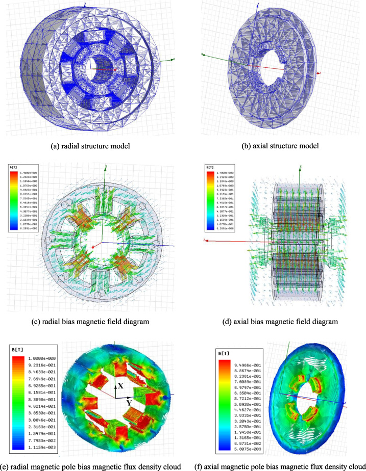
Diagram of simulation model and result.

Figure 4(c,d) show the magnetic line of force only in the bias magnetic field. It can be seen from the figure that the permanent magnet provides the bias magnetic field as the magnetomotive force source. Magnetic lines of force go through the air gap from the permanent magnet pole to the rotor core and then split into two paths. One part of magnetic line of force goes through the control pole and the radial stator to form a radial closed magnetic circuit. The other part goes through the axial stator pole and the outer magnetizer to form the axial closed magnetic circuit, which is consistent with the theoretical analysis. Figure 4(c–f) show the magnetic flux density of the radial and axial magnetic poles when the rotor is in the center and only the bias magnetic field is present. The magnetic flux density of the four permanent magnetic poles is equal, and also the magneticflux density of the four control poles, which are smaller than magnetic flux density at permanent magnetic pole. The magneticflux density at the magnetic poles on both sides of the axial direction is also equal.

5.2. Force/current curve and force/displacement curve

In order to verify the bearing capacity of the permanent magnet biased magnetic bearing in the whole displacement range and the current range, the performance curve of magnetic suspension force is obtained by using the magnetic circuit analysis and Ansoft. Figure 5(a,b) shows the force/current curve of the equilibrium position. The solid line is the calculation results and the dashed line is the FEA results. The calculation result of radial force/current coefficient and axial force/current coefficient is 110.86 N/A, 102.85 N/A, respectively. It can be seen that the linearity of the force/current curve is very good near the equilibrium position. When the current is less than 1.0 A, the results of FEA are very close to the calculation results. The variation between the calculation result and the FEA result is increased with the increasing current. In the simulations, considering the magnetic flux leakage and core reluctance, the mean errors were 5.07% and 4.11%, respectively.

Fig. 5.

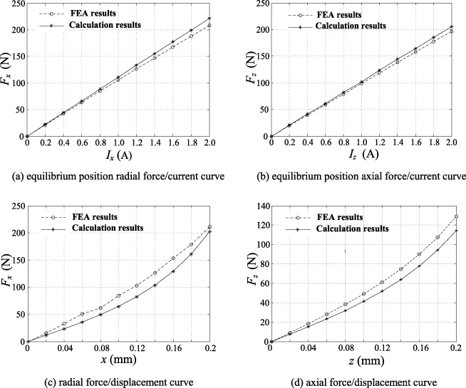
Equilibrium position force/current curve and force/displacement curve.

Figure 5(c,d) is the force/displacement curve. The dashed line is the FEA results and the solid line is the calculation results. It can be seen that the trend of calculations were consistent to analytical aligns with the finite element calculations. Although the force/displacement relationship is nonlinear in the whole range, the linear relationship is shown near the equilibrium position and the finite element calculations are close to that of the calculations as analytical. When the offset displacement is large, the calculation results are smaller than the FEA results and the average error is about 25.78% and 17.65% respectively. The reason for the relatively large error is that the passive bearing capacity is not taken into account in the calculation as analytical. When the rotor deviates from the equilibrium position, the suction force of four permanent magnetic poles on the rotor is not exactly the same. The suction force of the permanentic pole on the side of rotor increases, while the suction force of the permanent magnetic pole on the opposite side of rotor decreases, so that the simulated value is larger than the theoretical result.

In order to observe the distribution of magnetic flux density in each air gap more intuitively, the simulation results obtained in Ansoft include air gap magnetic flux density curve, which go along the air gap one circle. The abscissa d represents the length of the air gap simulation curve, and the ordinate B is the air gap magnetic flux density at the corresponding position. Figure 6(a) is the schematic diagram of the positon of the radial air gap simulation curve. Figure 6(b) is the magnetic flux density curve of the radial air gap. There are three curves in Fig. 6(b), and the blue curve is the air gap magnetic flux density curve with only the bias magnetic field. It can be seen that the magnetic flux density at the air gap of the four permanent magnetic poles is 0.84 T, and the magnetic flux density at the air gap of the foure control poles is 0.52 T. The red curve is the curve of air gap magnetic flux density, which exists in the bias magnetic field. And the excitation magnetic motive force with 100 A-turns is added to the +X direction. Air-gap magnetic flux density on +X direction has superimposed to 0.7 T, and air-gap magnetic flux density on −X direction has reduced to 0.38 T. The black curve is the curve of air gap magnetic flux density which exists in the bias magnetic field. And with the excitation magnetic motive force with 200 A-turns, the radial bearing capacity reaches the maximum. Air-gap magnetic flux density on +X direction has increased to the maximum 1.1 T and air-gap magnetic flux density on −X direction has reduced to zero. It can be seen from the figure, with the increasing excitation current on X direction, the magnetic flux density at air gap of Y direction stays unchanged. In this case, the radial bearing capacity of the rotor reaches the maximum of 215.91 N, which is slightly smaller than the design target value. The error is 6.13%. The reason is that the finite element simulation considered the magnetic flux leakage and core reluctance, etc.

Fig. 6.

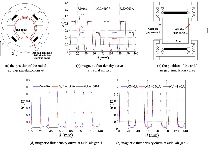
Radial and axial air gap simulation.

Figure 6(c) is a schematic diagram of the position of axial air gap simulation curve. Curves 1 and 2 are two circular curves located in the middle of the axial air gap. Figure 6(d) is the magnetic flux density curve of the axial air gap 1, and Fig. 6(e) is the magnetic flux density curve of the axial air gap 2. The blue curve is the air gap magnetic flux density curve with only the bias magnetic field. The magnetic flux density at air gap 1,2 are both 0.52 T. The red curve is the curve of the air gap magnetic flux density, which exists in the bias magnetic field and the excitation magnetic motive force with 100 A-turns is added to the +Z direction. The magnetic flux density at air gap 1 is reduced to 0.24 T, and the magnetic flux density at air gap 2 is increased to 0.8 T. The black curve is the air gap magnetic flux density curve, which exists in the bias magnetic field and the excitation magnetic motive force with 190 A-turns is added to the +Z direction. In this case, the axial bearing capacity reaches the maximum, and the magnetic flux density distribution of air gap 1 is simulated. Magnetic flux density at air gap 1 has reduced to zero, and magnetic flux density at air gap 2 has increased to 1.03 T. It can be seen from the analysis of Section 3.3 that the axial bearing capacity of the rotor reaches the maximum value of 196.35 N, which is smaller than the design target value. The error is 6.5%, and the cause of this error is the same as that of the radial error.

6. Experiment results

6.1. Test rig

In this paper, the schematic block diagram of test rig shown in Fig. 7(a) mainly consists of mechanical devices and control systems. The mechanism includes a rotor, a stator of HMB, a backup bearing and a self-aligning ball bearing, which can compensate for shaft and bearing dislocation and shaft deflection error. The control system includes sensors, controllers and amplifiers.

Fig. 7.

Schematic block diagram and photo of three-degree-of-freedom HMB.

Figure 7(b) shows experimental system, which includes mechinery, sensor board, PID controller, PC, power amplifier, switching power supply and so on.

6.2. Measurement of bearing capacity

When designing a permanent magnet bias magnetic bearing, the bias flux density is half of the saturated magnetic flux of the magnetic material, which can make full use of permanent magnets. When the maximum current flows into the control coils, the control flux density is just half of the saturated magnetic flux. The control magnetic field and the bias magnetic field offset to zero, meanwhile the superposition of control magnetic flux and bias magnetic flux achieves saturated magnetic flux. And the HMB bearing capacity reaches the maximum at this time. In this paper, the bearing capacity reaches the theoretical maximum bearing capacity when 2 A current flows into the control coils, and the bearing capacity test is required to verify the theory. The main principle of the test is as follows. In the radial or axial direction of the rotor, a spring dynamometer is used to measure the value of the bearing capacity. And then slowly add the load until the current reaches 2 A or instability. The reading obtained from spring dynamometer indicates the actual maximum bearing capacity at this time.

The force measuring device is shown in Fig. 8. During the test, the loaded (radial and axial bearing capacity should be measured separately) gradually added to the rotor. During loading process, the variation of current are observed to prevent the sudden unstable of the rotor, which will result in inaccurate measurement. When the rotor is unstable or the control current reaches the maximum design value, the value of spring dynamometer was record, which is the actual maximum capacity of the magnetic bearing. After measuring the value for 5 times, the average is calculated to reduce the measurements error and other random noise interference.

Fig. 8.

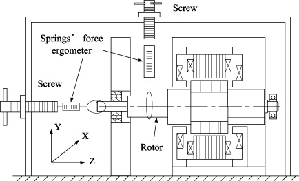
Schematic diagram of the force measuring device.

Table 3 shows the maximum bearing capacity of HMB. It can be seen from the table that the finite element simulation values and theoretical calculations are larger than the experimental values. This is because that rotor is already unstable when the radial and axial currents in the test have not reached the maximum current 2 A in the test. The maximum bearing capacity is the value of the spring dynamometer at the time of instability. When the rotor is instable, the difference between the finite element simulation values and test values of bearing capacity is relatively large. The error of radial maximum bearing capacity is 6.96% and the error of axial maximum bearing capacity is 8.37%.

Table 3

Permanent magnet biased magnetic bearing maximum load capacity measurement table

Name	Radial bearing capacity/N	Axial bearing capacity/N
Design goals	230	210
Theoretical calculated value	221.7	205.7
Finite element simulation value (instability)	204.2	185.5
Test value	190	170
Relative error rate of finite element simulation value and test value	6.96%	8.37%

7. Conclusions

(1) A novel radial-axial HMB structure is proposed. The equivalent magnetic circuit diagram of the novel HMB is established, considering the influence of magnetic flux leakage and core reluctance on magnetic flux. Based on Kirchhoff’s law, the mathematic model is built, and the formula of bearing capacity is obtained.

(2) The HMB is designed to achieve the maximum bearing capacity. The function between current and displacement of magnetic suspension force is obtained by calculating magnetic reluctance of various parts of the investigated HMB.

(3) The magnetic field of the HMB is simulated and analyzed. And the theoretical analysis and parameter design has been verified by analyzing the magnetic flux density curve at the air gap.

(4) The bearing capacity measurement results show that the experimental values of radial and axial maximum bearing capacity are basically consistent with the theoretical predictions.

Footnotes

Acknowledgements

The authors gratefully acknowledge the support from the Natural Science Foundation of Jiangsu province, China (BK20161486), and from the Fundamental Research Funds for the Central Universities (NS2016053) as well as the Open Project Program of Jiangsu Key Laboratory of Large Engineering Equipment Detection and Control (JSKLEDC201502).

References

Schweitzerand

and Maslen

, Magnetic Bearings: Theory, Design, and Application to Rotating Machinery, Springer-Verlag, Berlin, Heidelberg, 2009.

Anantachaisilp

and Lin

Z.L.

, Fractional order PID control of rotor suspension by active magnetic bearings, Actuators 6(1) (2017), 4, Multidisciplinary Digital Publishing Institute.

Wang

X.G.

Zhao

and Hou

L.L.

, Structural design and performance analysis of a new type of axial magnetic bearings with multi-ring redundant structure in circular direction, International Journal of Applied Electromagnetics and Mechanics 55 (2017), 373–390.

Cheng

Chen

Zeng

H.Y.

Wang

X.G.

and Zhou

R.G.

, Reconfiguration rules for loosely-coupled redundant supporting structure in radial magnetic bearings, International Journal of Applied Electromagnetics and Mechanics (2016), 91–106.

Bouaziz

Hentati

Cholley

J.Y.

and Haddar

, Vibrations monitoring of high speed spindle with active magnetic bearings in presence of defects, International Journal of Applied Electromagnetics & Mechanics 49(2) (2015), 207–221.

Fang

J.C.

Sun

J.J.

Liu

and Tang

J.Q.

, A novel 3-DOF axial hybrid magnetic bearing, IEEE Transactions on Magnetics 46(12) (2010), 4034–4045.

Peng

and Fang

J.C.

, High-precision control for double-gimbal magnetically suspended control moment gyro via composite anti-disturbance control, Proceedings of the Institution of Mechanical Engineers, Part G: Journal of Aerospace Engineering 229(7) (2015), 1183–1193.

Prince

O.A.

Y.F.

and Wu

H.C.

, Design and analysis of a flywheel supported by hybrid magnetic bearing, Research Journal of Applied Sciences, Engineering and Technology 12(1) (2016), 1–8.

J.T.

Zhu

H.Q.

and Zhao

C.Y.

, Radial force-current characteristic analysis of three-pole radial-axial HMB, in: Vehicle Power and Propulsion Conference (VPPC), 2016 IEEE, IEEE, 2016, pp. 1–6.

10.

Cheng

S.B.

Olles

M.W.

Burger

A.F.

and Day

S.W.

, Optimization of a hybrid magnetic bearing for a magnetically levitated blood pump via 3-D FEA, Mechatronics 21(7) (2011), 1163–1169.

11.

Hou

E.Y.

and Liu

, Investigation of axial carrying capacity of radial hybrid magnetic bearing, IEEE Trans. Magn. 48(1) (2012), 38–46.

12.

Imoberdorf

Zwyssig

Round

S.D.

and Kolar

J.W.

, Combined radial-axial magnetic bearing for a 1 kW, 500,000 rpm permanent magnet machine, in: Twenty Second IEEE Applied Power Electronics Conference, USA, IEEE, 2007, pp. 1434–1440.

13.

Mei

, Fundamental Research on Hybrid Magnetic Bearings, Ph.D. Dissertation, Nanjing: Nanjng University of Aeronautics and Astronautics, 2008.

14.

Sortore

C.K.

Allaire

P.E.

Maslen

E.H.

Permanent magnet biased magnetic bearings-design, construction and testing, in: 2nd International Symposium on Magnetic Bearings, Japan, 1990, pp. 175–182.

15.

and Jin

, Research on a low power consumption six-pole heteropolar hybrid magnetic bearing, IEEE Transactions on Magnetics 49(8) (2013), 4918–4926.

16.

Okada

Kovanayi

and Kakihara

, New concept of miracle magnetic bearings, in: 9th International Symposium on Magnetic Bearings, Lexington, Kentucky, 2004, pp. 89–95.

17.

Filatov

and Hawkins

, Comparative study of axial/radial magnetic bearing arrangements for turbocompressor applications, Proceedings of the Institution of Mechanical Engineers, Part I: Journal of Systems and Control Engineering 230(4) (2016), 300–310.

18.

Zhao

X.S.

, Research on Permanent Magnet Biased Magnetic Bearing, Ph.D. Dissertation, Nanjing: Nanjing University of Aeronautics and Astronautics, 2011.

19.

Okada

Sagawa

Suzuki

and Kondo

, Development and application of parallel PM type hybrid magnetic bearings, in: 11th International Symposium on Magnetic Bearings, Nara, Japan, 2008, pp. 18–24.

20.

Zhao

Deng

and Wang

, Parameter design realization of permanent magnet biased heterploar radial magnetic bearing, Transactions of China Electrotechnical Society 7 (2012), 131–159.

21.

Fang

and Sun

, New permanent magnet biased radial magnetic bearing in magnetic suspending flywheel application, Journal of Beijing University of Aeronautics and Astronautics 32(11) (2006), 1304–1307.

22.

Huang

Zhu

Xie

and Chen

, Parameter design analysis for two-degrees of freedom radial hybrid magnetic bearings, China Mech. Eng. 18(10) (2007), 1143–1146.

23.

Kenny

and Palazzolo

A.B.

, Single plane radial, magnetic bearings biased with poles containing permanent magnets, ASME J. Mech. Des. 125(1) (2003), 178–185.

24.

Lee

A.C.

Hsiao

F.Z.

and Ko

, Analysis and testing of magnetic bearing with permanent magnets for bias, JSME International Journal 37(4) (1994), 774–782.

25.

Lee

A.C.

Hsiao

F.Z.

and Ko

, Performance limits of permanent-magnet-biased magnetic bearings, JSME International Journal 37(4) (1994), 783–794.

26.

Hawkins

and McMullen

, An AMB energy storage flywheel for industrial applications, J. Japan Soc. Appl. Electromagn. 16(4) (2008), 287–293.

27.

McMullen

P.T.

Hawkins

L.A.

Huynh

C.S.

and Dang

D.R.

, Design and development of a 100 kW energy storage flywheel for UPS and power conditioning applications, in: The 24th International PCIM Conference, Nuremberg, Germany, 2003.

28.

Huang

Zhao

G.Z.

Nian

and He

Y.K.

, Modeling and design of permanent magnet biased radial-axial magnetic bearing by extended circuit theory, in: Proceeding of International Conference on Electrical Machines and Systems, Seoul, 2007, pp. 1502–1507.

29.

Mei

Deng

Z.Q.

and Zhao

X.S.

, Parameter design of hybrid axial-radial magnetic bearing based on magnetic flux calculation, Transactions of China Electrotechnical Society 29(24) (2009), 115–121.

30.

X.J.

Palazzolo

Tingey

Han

McMullen

and Wang

Z.Y.

, Shaft-less energy storage flywheel, in: ASME 2015 9th International Conference on Energy Sustainability, California, 2015, ES2015-49079.

31.

X.J.

Anvari

Palazzolo

Wang

Z.Y.

and Toliyat

, A utility-scale flywheel energy storage system with a shaftless, hubless, high-strength steel rotor, IEEE Transactions on Industrial Electronics 65(8) (2018), 6667–6675.

32.

Calnetix’s Powerflux^TM Active Magnetic Bearings, Availabe from: www.calnetix.com.

33.

McMullen

P.T.

Huynh

C.S.

and Hayes

R.J.

, Combination radial-axial magnetic bearing, in: The 7th International Symposium on Magnetic Bearings, ETH Zurich, Switzerland, 2000, pp. 287–293.