
Abstract
In this paper we present a-priori model reduction technique that enables to take full advantage of the periodicity existing in the stator and rotor geometrical structures of electrical machines in order to reduce the computational time. Firstly, a change of basis is performed by applying two distinct discrete Fourier transformations on the stator and rotor periodic structures independently. Secondly, the Schur complement is introduced in the new spectral basis, to allow a parallel solving of the resulting block-diagonal matrix systems. Moreover, the using of a matrix-free Krylov method based on the conjugate gradient solver has verified an efficient solving of the equation system associated to the stator-rotor interface. Furthermore, in the peculiar case of balanced supply conditions, a model order reduction can be carried out by considering only the dominant discrete Fourier transform components. This model reduction approach is applied on a buried permanent magnet machine and has successfully shown its efficiency under balanced and unbalanced conditions.
Keywords
Introduction
The main challenge in numerical modeling is to search for a compromise between a good accuracy and a reduction in memory storage and computing time requirements. To advance towards this objective, the model reduction techniques become increasingly used, and this especially in electromagnetic fields computation. These can be a-posteriori model reduction techniques like proper orthogonal decomposition [1] and perturbation zooming methods [2] or a-priori reduction techniques like the ones dealing with the magnetic symmetry or further geometrical periodicity exhibited in most rotating electrical machines [3–5].
The difficulties encountered in the a-posteriori techniques remain the determination of a well-conditioned reduced basis as in the case of the model order reduction methods [6] and the association of equitable boundary conditions as in the case of most subdomain reduction methods [7]. In the a-priori techniques, we can list likewise several limitations. In fact, the reduction technique using magnetic symmetries takes advantage of the symmetrical magnetic flux lines distribution. Let’s take the example of a permanent magnet machine with N s stator teeth and 2p rotor permanent magnets. In case of a kind of consistent distribution of the 2p permanent magnets with respect to the N s stator teeth, which means a greatest common divisor (GCD) of N s and 2p greater than 1, the modeling of a single 1∕GCD (N s , 2p) section is enough to determine effectively the full model solution by simple periodic or anti-periodic relationships [8]. Nevertheless, such magnetic symmetry can be exploited only in case of balanced supply conditions. The geometrical periodicity on the other hand, considers only the materials permeability regardless the sources distribution and the supply regime whether it is under balanced or unbalanced conditions. In the case of a buried permanent magnet machine (BPMM) for example with N s and N r stator and rotor teeth respectively, one can model only 1∕GCD (N s , N r ) machine section [9]. The modeling of this single elementary section which can regenerate the full geometrical model by simple rotation transformations, is enough to determine the full model solution if one uses the group representation theory [3,4]. However, such classical exploitation of the geometrical periodicity does not allow to take advantage of the total geometrical periodicity existing separately in the stator and rotor domains.
To tackle this issue, we investigate in this paper a-priori model reduction technique that takes full advantage of the geometrical periodicities existing in the stator and rotor structures, and goes further than the classical approach by allowing to only model a single 1∕N s elementary section of the stator with a single 1∕N r elementary section of the rotor. When it deals with the symmetrical properties of the block circulant matrices, this reduction technique is akin to the group representation theory [10,11] and can be applied regardless of the sources distribution. In a first step, this reduction technique is implemented by means of two distinct discrete Fourier transforms (DFT) applied to the two distinct periodic structures of the stator and rotor domains. In a second step when the rotor motion is taken into account, the Schur complement is used to solve the matrix system obtained from the coupling of both stator and rotor problems [12,13]. We should denote that the continuous rotor motion is performed using the spatial Fourier interpolation method (SFIM) [14,15] which is an extension of the locked step method [16]. We should also point out that the presented approach in this paper is applied to reduce the computational time in the case of linear finite element analysis. In fact, the homogeneous magnetic property of the materials with a linear behavior retains effectively the geometrical model periodicity. Nevertheless, such geometrical periodicity is broken in the case of a non-linear analysis. In the non-linear case, some techniques have been proposed to keep the block circulant property by using iterative algorithms based on the fixed-point technique or the transmission-line method. Such techniques allow not only to apply the DFT but also to account for the non-linearity by introducing an additional fictitious source term on the righthand side of the equation system [5,17].
The proposed model reduction technique is applied to study a 9 teeth/8 poles BPMM. In fact, this particular machine does not present neither any magnetic symmetry nor any consistent geometrical periodicity between the stator and rotor structures, and thus requires a full modeling with the classical approach.
Classical exploitation of geometrical periodicity in the finite element (FE) modeling
Linear magnetostatic FE modeling
Let us consider a domain 𝛺 of boundary 𝛤 (𝛤 = Γ1 ∪ Γ2 and
To solve the previous problem, the magnetic potential A (B = curl A) is introduced. The unicity of A is imposed with the addition of a gauge condition; this can be a Coulomb gauge which is implicitly verified in our case of 2D modeling. Adding now the magnetic potential to (1) and (2), the new resulting equation to solve will be:
Let us generalize and consider the case of an electromagnetic device made up of N periodic sections (Fig. 1). We suppose that the periodicity holds only on the permeability but not on the source produced by the currents or the residual magnetic flux density.
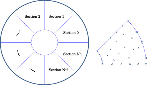
Full model (left), modeling of one elementary section: the crossed points represent the inner nodes, the round points represent the ones common with the previous section and the squared points represent the ones subjected to Dirichlet conditions (right).
Since the partial differential equation (4) cannot be determined analytically, solving technique by FE discretization is used. Therefore, to take into account the geometrical periodicity we have to fulfill a numerical periodicity homologous to the geometrical one. To do so, we impose that all the sections are discretized by the same mesh and have thus the same number and distribution of nodes. To achieve this, it is sufficient to discretize only the elementary periodic section, as the one presented in Fig. 1, in such a way that the full model can be deduced by a simple concatenation of the elementary model. n is supposed to be the number of the degrees of freedom in each section. It represents the total number of inner nodes excepting in the one hand, the nodes located on the boundary where a Dirichlet condition is imposed and in the other hand, the ones located on the common side with the previous section (Fig. 1).
Now, the geometrical periodicity on the material characteristics of the N sections is in agreement with the numerical discretization periodicity. Taking into account the latter, and applying a 2D FE formulation of the linear magnetostatic problem described by the equation (4), a linear system of matrix equations is obtained:
In this section, we will spell out the incidence of the geometrical periodicity on the model reduction. In fact, since [S
c
] in (6) is a block circulant matrix, it can be decomposed, by using a DFT, under the following form [18,19]:
Finally, in the spectral basis the new system to solve can be deduced combining (6) and (7):
Moreover, solving these N independent subsystems can be done using a parallelization process. Accordingly, it will lead to a considerable reduction of the computational time. Finally, we can deduct from (12) the scattered full model solution on the N different sections; it is given by [A] = [W][Z].
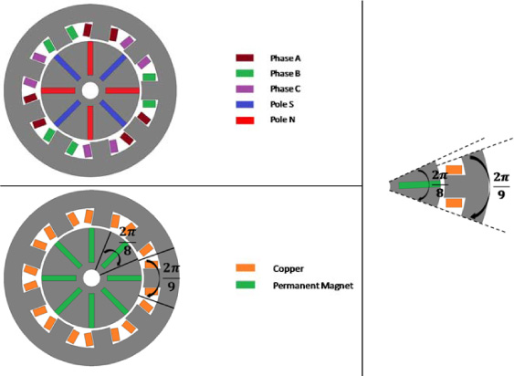
The 9/8 BPMM: highlighting the different sources (top left), considering the permeability of materials regardless of sources (bottom left), the two elementary cells of the stator and rotor domains (right).
Now, let’s apply the previously described method exploiting the geometrical periodicity on the modeling of an electrical machine example. We take therefore a BPMM consisting of N s = 9 stator teeth wound by a three phase winding, and 2p = 8 rotor poles (Fig. 2). From the point of view of the distribution of the magnetic field lines, even when the stator windings are fed with a balanced supply conditions, we can expect that this machine will not present any magnetic symmetry since the GCD between N s and 2p is equal to 1 (GCD (N s = 9, 2p = 8) = 1) [8,9]. Therefore, we can denote that, for reasons of simplifications, the stator windings can be left unloaded. On the other side considering now the materials permeability point of view regardless the excitation sources distribution, no global consistent stator-rotor geometrical periodicity is exhibited since the rotor salient structure represents N r = 8 rotor teeth -due to the presence of 8 buried permanent magnets- which means in fact that GCD (N s = 9, N r = 8) = 1 [9]. Based on the forgoing, there is neither a magnetic symmetry nor a classical consistent geometrical periodicity as the one described in Fig. 1 and therefore the full machine should be considered for a magnetostatic finite element modeling. However, we can distinguish two independent geometrical periodicities in the stator and rotor structures regardless of the sources distribution (current sources and residual magnetic flux densities). (Fig. 2). Consequently, we find 9 identical periodic cells in the stator involving each a single stator tooth and 8 identical periodic cells in the rotor representing each one rotor pole. These two elementary cells are represented in Fig. 2. In the next section 3, we will show how we can totally exploit such independent periodicities existing in the most stator and rotor domains of rotating electrical machines. This will be applied to study the 9/8 BPMM considered example, later in Section 4.
Methodology
We suppose now the case of a rotating electromagnetic device, consisting of a fixed stator and a movable rotor, and disposing – as it is in the general case – of a distinct periodicity in the stator and the rotor geometrical structures.
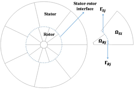
Full model of a rotating electromagnetic device: The marked fictive interface separates the fixed part (stator) from the rotating part (rotor) (left), modeling of one elementary section (right).
We assume to perform the rotor motion using the SFIM [14,15] which is an extension of the locked step method [16]. To do so, the presence of a fictive interface between the stator and the rotor is assigned (Fig. 3). Since the full model of the device represents N s identical periodic sections in the stator and N R identical periodic sections in the rotor, the geometrical periodicity, as it has been developed before, is now exploited in the stator and rotor domains separately; the elementary model is consisting of one 1∕N s elementary section of the stator and another 1∕N r elementary section of the rotor (Fig. 3).
In Fig. 3, we can notice that in each elementary section of the electromagnetic device we can distinguish the elementary stator domain 𝛺
si
(0 ≤ i ≤ N
s
− 1) whose number of degrees of freedom is n
s
from the one of the rotor domain 𝛺
rj
(0 ≤ i ≤ N
r
− 1) whose number of degrees of freedom is n
r
. The stator-rotor interface, where the motion is considered is duplicated to create dual Γ
si
and Γ
rj
separation interfaces which belong respectively to 𝛺
si
and 𝛺
ri
. The relationship between the discretization nodes of the different interfaces Γ
si
and Γ
rj
allows, according to the locked steps method [16] or the SFIM [15], to consider the rotor motion. Based on the foregoing, we can summarize that there are N
s
periodic sections in the stator, the degree of freedom of each is n
s
and N
R
periodic sections in the rotor, and the degree of freedom of each is n
r
. The use of the geometrical periodicity which makes it possible to construct the stator and the rotor full models of the electromagnetic device independently by concatenation of the stator and rotor elementary models leads to obtain, according to the equations (5) and (6), the following redundant overdetermined system to solve:
Since the problem is treated independently within the stator and the rotor subdomains, the matrix system (14) is overdetermined thanks to the duplicated nodes of the stator-rotor interface; the equations relating to these nodes are written twice: the first for their relation with the inner nodes of the stator and the second for their relation with the inner nodes of the rotor. [S
cs
] and [S
cr
] are two block circulant matrices linked to stator and rotor geometrical subdomains respectively. [A
s
] and [A
r
] which are respectively of size ([N
s
× n
s
] × 1) and ([N
s
× n
r
] × 1), represent the set of nodal magnetic potential unknowns in the stator and the rotor, and [F
s
] and [F
r
] are the source terms. The vectors [A
s
], [A
r
], [F
s
] and [F
r
] are given with their following explicit forms:
According to (7), the block circulant matrices [S
cs
] and [S
cr
] can be decomposed, using two distinct DFT, under the following forms:
Combining now the matrix system (14) with the equations in (16), we obtain in the spectral basis the new system to solve:
Since [S
Δs
] is a block diagonal matrix, we have therefore N
s
independent sub-systems of size n
s
each and since [S
Δr
] is a block diagonal matrix, we have likewise N
r
independent subsystems of size n
r
each:
To properly solve the overall problem consisting of these different independent subsystems in the stator and the rotor domains, they must be coupled together at the stator-rotor interface. To do so, we have to express the different [(Z
Γ
r
)
j
] as functions of the different [(Z
Γ
s
)
i
]. In other words, where [Z
Γ
s
] and [Z
Γ
r
] are respectively the set of [(Z
Γ
s
)
i
] and [(Z
Γ
r
)
j
] we must express [Z
Γ
r
] in terms of [Z
Γ
s
]. This can be done by performing the rotor motion using the SFIM. It allows considering any rotation angle θ of the rotor and not only the discrete few angle steps given by θ
m
= mΔθ, where
Unlike the locked step method which takes into account discrete rotation steps [16], the SFIM allows therefore to take into account the continuous rotor motion. Assuming that [A
Γ
S
] = [(A
Γ
s
)0≤i≤N
s
−1] and [A
Γ
r
] = [(A
Γ
r
)0≤j≤N
r
−1] are the vectors of total magnetic potential unknowns on the stator-rotor interface in the stator and rotor side respectively, the SFIM consists in expressing the DFT of both vectors [A
Γ
S
] and [A
Γ
r
] under the following equation [15]:
Now, given that [W
F
] of size (m
D
× m
D
) is the transformation matrix corresponding to the DFT based on the local discretization of the stator-rotor interface, the vectors [Z
F
Γ
s
] and [Z
F
Γ
r
] are given by the following equations:
We should denote furthermore that the vectors [A
Γ
s
] and [A
Γ
r
] can be expressed in function of their DFT vectors [Z
Γ
s
] and [Z
Γ
r
] by the following expressions respectively:
Combining now the equations (24), (26), (27), (28) and (29) leads to the following expression:
In the spectral basis, [Q (θ)] is the matrix linking the interface variables of the stator to those of the rotor at the rotor position θ and then defining the continuous rotor motion. The matrix [D (θ)] being diagonal, therefore the matrix [W F ][D (θ)][W F ]−1 is circulant. However, in our case of a non-consistent periodicity in the stator and the rotor, [W Γ s ] ≠ [W Γ r ], and therefore the matrix [Q (θ)] = [W Γ r ]−1[W F ][D (θ)][W F ]−1[W Γ s ] is not a block diagonal matrix. In the following and for reasons of simplification we will replace [Q (θ)] by [Q].
The matrix [Q] being not a block diagonal matrix, each sub-vector [(Z Γ r ) j ] must be expressed as a function of all the vectors [(Z Γ s ) i ]. This will not have any advantage if one wants to have independent subproblems resulting from the stator-rotor coupling. For this reason, we will proceed to tackle this issue by the use of the Schur complement method.
The application of the Schur complement actually requires a particular form of the matrix to be solved. This indeed requires a reordering of the variables in the vectors [Z
s
] and [Z
r
]. After such reordering of the variables, these two vectors will be written henceforth by the following expressions:
Using the expressions of the vectors [Z
s
] and [Z
r
] in (33) by separating the variables associated within the inner domain from those located on the interface, the matrix system in the equation (19) can be now written in the following form:
Using now the equation (35) in (34), and multiplying by the transposed matrix of [P] in order to add the contribution from both sides of the stator-rotor interface, the new matrix equation system that yields will be therefore:
This particular type of matrix system equation can be solved using the Schur complement [12,13]. This can be done by using a simple substitution method. Let’s rewrite therefore the first and the second equation in (36) by determining the expressions of [Z
ss
] and [Z
rr
] in terms of [Z
Γ
s
] as the following:
Now replacing [Z
ss
] and [Z
rr
] by their values given by the equations in (37), in the third equation of the full system (36), we will obtain therefore the following system to solve whose size is equal to the number of nodes on the interface, and which is very small in comparison with the initial full problem.:
At the end, the Schur complement will lead us to the following system that can be solved in the opposite direction now with a back substitution method:
The determination of [Z
Γ
s
] by solving the system (38) in a first step allows us to calculate [Z
Γ
r
] using the equation (32) and to determine [Z
ss
] and [Z
rr
] in a second step and this by solving respectively the two following matrix equations:
We should denote that, to solve (38), we can avoid the implicit calculation of the matrix [S sr ]. This can be done using a matrix-free Krylov method based on the conjugate gradient solver [21]. It is an iterative method that does not deal with the direct solving of the system (38) but with an iteration process of matrix-vector multiplications. At each iteration, the matrix [S sr ] is multiplied by the kth iteration vector denoted [y k ].
Since [S Δss ] and [S Δrr ] are block-diagonal matrices with N s and N r matrix blocks respectively; the system (40) will lead to (N s + N r ) independent subsystems that can be solved effectively in a parallel computation process. Moreover, this parallel computation can be used also to solve for [S Δss ]−1[C ss ] and [S Δrr ]−1[C rr ] within the calculation of [C sr ] and to solve for [S Δss ]−1[S ΔΓ s s ][y k ] and [S Δrr ]−1[S ΔΓ r r ][Q][y k ] within each conjugate gradient solver for the solution [Z Γ s ] of the system (38). Henceforth, the solving of the matrix system (39) using a back substitution method combined with a parallelization process can lead to an effective acceleration in the computational time which will be verified in the following example.
To prevent a repetitive direct solving technique, we recommend the use of an implicit LU decomposition. The LU decomposition uses a backward and forward solving i.e. triangular solving and has verified therefore a more efficient calculation time. If we consider that (S Δss ) i and (S Δrr ) j are the ith (0 ≤ i ≤ N s − 1) and the jth (0 ≤ j ≤ N r −1) matrix blocks of the block diagonal matrices [S Δss ] and [S Δrr ] respectively, we can write: (S Δss ) i = (L ss ) i × (U ss ) i and (S Δrr ) j = (L rr ) j × (U rr ) j . These LU decomposition matrices are calculated one time and are stored; this avoids a significant waste of the computational time in the repetitive direct solving technique that will be requested for example in the conjugate gradient iterations in (38). All these steps to solve the system (39) can be summarized in the following diagram in Fig. 4. We should denote that the boxes with dashed borders represent the ith and the jth systems of the N s and N r systems respectively, that could be solved in a parallel process. Furthermore, and for reasons of simplification, the conjugate gradient solver box is represented only by the matrix- vector multiplication of the matrix [S sr ] with the iterative vector [y k ] at the kth iteration.
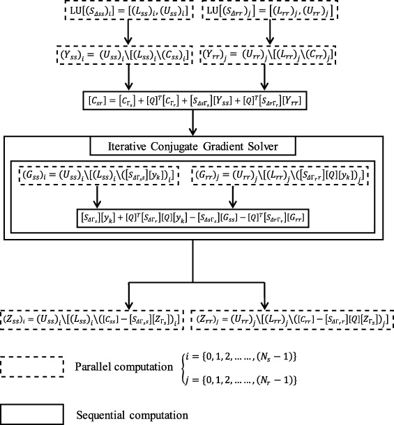
Diagram showing the different solving steps and highlighting the parallel computational processes presented by the boxes with dashed borders.
The application example is a 9/8 BPMM (Fig. 5). It consists of 9 stator teeth and 8 rotor permanent magnets. As we have mentioned in Section 2, there is neither an obvious magnetic symmetry nor a whole consistent geometrical periodicity in this studied machine. As a matter of fact, the full machine should be modeled in the classical approach. However, the stator and the rotor represent two different geometrical periodic structures. In fact, from an elementary 1/9 section of the stator and an elementary 1/8 section of the rotor we can generate the full model of the machine. Therefore, to exploit the total geometrical periodicity as we have noticed in Section 2, the elementary periodic cell in the stator turns out to be only one stator tooth and that of the rotor turns out to be only one permanent magnet (Fig. 5).
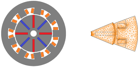
The BPMM 9/8 (left), Mesh of the elementary modeled sections: elementary 1/9 stator section and elementary 1/8 rotor section (right).
We should denote that the 2D spatial mesh of the elementary cell is made of n s = 738 nodes in the stator section and n r = 512 nodes in the rotor section, and that for reasons of simplifications, as we have mentioned in Section 2, the stator phases are left unloaded. From the mesh of one elementary cell we have reconstructed a full FE model (reference) that we have compared to the reduced model. The exploitation of the geometrical periodicity makes it possible to switch effectively from the large FE system into 9 independent subsystems in the stator, 8 independent subsystems in the rotor and one system representing the coupling of the stator-rotor nodes on the connecting interface.
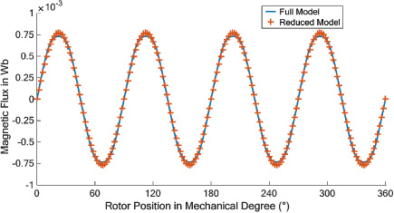
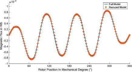
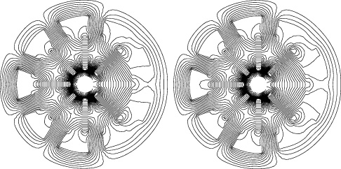
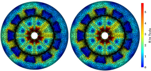
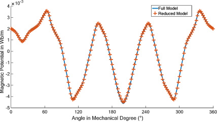
The first application is the case of a balanced permanent magnet source distribution in the rotor while the stator winding is kept unloaded. In fact, we have verified that the reduced model solution matches largely the one of the reference full model. The post processing global quantity compared between both models is the magnetic flux flowing through a tooth coil (Fig. 6). The local quantities are the flux lines distribution (Fig. 7), the magnetic flux density (Fig. 8) and the magnetic potential calculated at the air gap level in function of the angular position (Fig. 9).
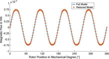
Magnetic flux through a tooth coil calculated with the reference full model and the reduced model.
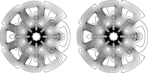
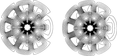
Flux lines distribution calculated with the reference full model (left) and the reduced model (right).
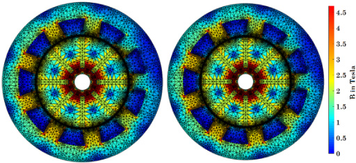
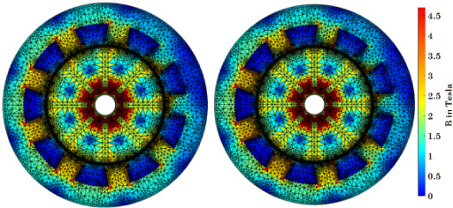
Flux density distribution calculated with the reference full model (left) and the reduced model (right).
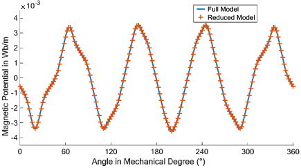
Magnetic potential in the air gap in function of the angular position calculated with the reference full model and the reduced model.
The flux lines, the flux density distributions and the magnetic potential are calculated at a given rotor position while the magnetic flux is calculated for a full rotor mechanical revolution. The conjugate gradient solver converges after 72 iterations with a stop criterium defined by a maximum residual error of 10−3. The speed up resulting from the transformation of the large system into the spectral basis system is 6 when using a sequential computation and 11 if we use a parallelization process. The errors between the full and the reduced models are 0.15% in the calculation of the magnetic flux and 0.3% for the air gap magnetic potential. This error is due to the use of a matrix-free krylov iteration method which is characterized by a maximum number of iterations linked to a stopping criterium that insures a minimum residual error.
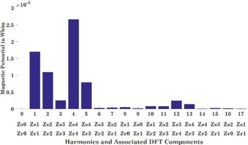
Each component of the stator and the rotor DFT components actually represents a given spectral content of the solution distribution in the stator and the rotor domain respectively (see Appendix B). According to (55) the harmonic spectrum of the stator and the rotor solution distribution can be projected to the corresponding DFT components as presented in Tables 1 and 2. The conjugate relationship between the different DFT components is explained in Appendix A. In our case, the distribution of the source in the rotor has a particular shape: it consists of 4 pairs of permanent magnets leading to a source distribution in such a way that the 4th harmonic is dominant. This can be verified by looking at the spectral representation of the magnetic potential distribution in the airgap (Fig. 10).
Harmonic content of the stator DFT components
Harmonic content of the stator DFT components
Harmonic content of the rotor DFT components
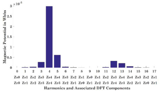
Spectral representation of the magnetic potential distribution at the air gap level with respect to the associated stator and rotor DFT components.
In Tables 1 and 2,
The results are in agreement not only with respect to the global quantity of the magnetic flux (Fig. 11) where the error does not exceed 1.8% but also regarding the local ones (Figs 12, 13, 14 and 15), but now with a slight low precision where the error considering the calculation of the magnetic potential in the air gap which is about 11% from the stator side (Fig. 14) and 14% from the rotor side (Fig. 15).
Magnetic flux through a tooth coil calculated with the reference full model and the reduced model with only Z s4 and Z r4.
Flux lines distribution calculated with the reference full model (left) and the reduced model with only Z s4 and Z r4 (right).
Flux density distribution calculated with the reference full model (left) and the reduced model with only Z s4 and Z r4 (right).
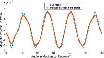
Magnetic potential in the air gap in function of the angular position calculated with the reference full model and the reduced model with only Z s4.
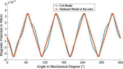
Magnetic potential in the air gap in function of the angular position calculated with the reference full model and the reduced model with only Z r4.
In this section we will study the case of an unbalanced regime characterized by a demagnetization defect of a permanent magnet in the rotor (Fig. 16). In this case, we can no longer speak about a particular distribution of the solution in the machine and thus of the dominance of a single spatial harmonic as it was the case in the balanced regime. Therefore, all the DFT components in the stator and the rotor domain have to be calculated. The conjugate gradient solver converges after 97 iterations with the same stop criterium, as in balanced conditions, defined by a maximum residual error of 10−3. The number of iterations until convergence is not the same in the case of balanced and unbalanced conditions since the convergence depends on the source vector. Now the speed-up is slightly smaller and it is about 5 in the case of a sequential computation of the problem and about 10.2 when we use the parallel computation. The solution calculated by the reduced model is compared to the one of a classical full model in the case of the demagnetization defect: they are in a good agreement as we can see in Figs 17, 18, 19, and 20.
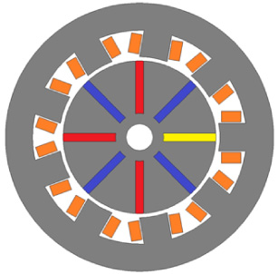
Demagnetization defect of a permanent magnet in the rotor.
Magnetic flux through a tooth coil calculated with the reference full model and the reduced model.
Flux lines distribution calculated with the reference full model (left) and the reduced model (right).
Flux density distribution calculated with the reference full model (left) and the reduced model (right).
Magnetic potential in the air gap in function of the angular position calculated with the reference full model and the reduced model.
The error does not exceed the 0.15% with respect to the calculation of the magnetic flux in a full mechanical revolution (Fig. 17) and the 0.3% with respect to the calculation of the magnetic potential in the airgap (Fig. 20).
The harmonic spectrum of the magnetic potential distribution in the airgap in Fig. 21 shows that this distribution is not governed by a single spatial harmonic but by different harmonics of considerable values. The solution in the stator and the rotor as well as the magnetic potential in the airgap are calculated separately in function of each stator and rotor DFT components and are represented in Figs 22 and 23.
Spectral representation of the magnetic potential distribution at the air gap level with respect to the associated stator and rotor DFT components.
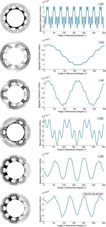
Flux lines distribution and air gap magnetic potential calculated in the stator by means of the different modes Z s0, Z s1, Z s2, Z s3 and Z s4.
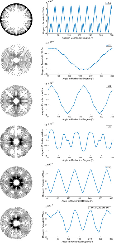
Flux lines distribution and air gap magnetic potential calculated in the rotor by means of the different modes Z r0, Z r1, Z r2, Z r3 and Z r4.
In this paper we have investigated a-priori model reduction approach based on the full exploitation of the spatial periodicity exhibited in the stator and rotor geometrical structures of the most rotating electrical machines. In fact, the use of the Schur complement has enhanced such exploitation of the geometrical periodicity by leading to solve in parallel the block diagonal matrix systems in the stator and rotor domains. Moreover, an efficient solving of the stator-rotor coupling system on the interface is carried out by means of the matrix-free Krylov method based on the conjugate gradient solver. A 9/8 BPMM is studied in balanced and unbalanced regimes; it has a particular geometrical structures where no magnetic symmetry neither a classical consistent geometrical periodicity can be used to reduce the FE modeling. However, using the presented model reduction approach, we have successfully managed to solve the matrix system with a speed up of about 6 in case of a sequential computation and 11 when we use a parallel process.
Furthermore, in the particular case of balanced supply conditions, we have verified a model order reduction of the FE model due to the DFT properties; only one DFT component that represent the prevailing harmonic of the solution distribution can be only solved for, which lead to an effective acceleration in the calculation time of about 11 within even a sequential computation of the matrix system.
Footnotes
Conjugate relationship between DFT components
Assuming the case of a vector X of dimension N given by the following form:
The DFT vector [Z] of [X] will be given by the following expression using the inverse DFT matrix [U]−1:
From the equations (42) and (43), the general term Z
m
of the vector [Z] will be given therefore by the following expression:
Let us first suppose the case where N, the number of samples is even, then the vector [Z] can be given by its general representation form:
Based on the equation (44), the expressions of both general terms
In the other case where the sampling number N is odd, the vector [Z] can be given its general representation form:
In the same way, based on the equation (44) the expressions of both general terms
Spectral content of DFT components
Let’s consider the case of a signal x (t) representing a sinusoidal function of frequency kf corresponding to the kth harmonic of a reference signal of frequency f. When this given kth harmonic signal whose mathematical representation is x (t) = A
k
sin(k2πft), is discretizing through a sampling frequency F
s
= N ∗ f, the sampling vector consisting of the N samples will be given by the following form:
Performing now in a following step, the DFT of the vector [X] which leads to the vector [Z] = [U
−1][X] whose general term, using equation (44), is given by the following expression:
We can show that this series in (54) will be not equal to zero if there exists an integer l such that:
In the excepted cases presented by the relation (55),