
Abstract
A method is proposed for the calculation of current density in a long solid metallic conductor placed in an external variable magnetic field. The external magnetic field is perpendicular to the conductor and constant on straight lines parallel to the conductor. The conductor is passive, connected to neither a voltage source nor a current source. It is assumed that the external magnetic field is quasi-stationary and is not affected by the magnetic field of the currents induced in the conductor under examination. The frequency of external field does not exceed 1 MHz and the displacement current is neglected. The proposed method enables the calculation of current density not only in the steady state but also in the case that the external field has an arbitrary time-dependent course. Results are given of the calculation of current density in conductors with symmetrical and unsymmetrical cross section, with constant and non-constant resistivity in the conductor cross section, for both homogeneous and non-homogeneous external steady-state sinusoidal field, and for switching the external sinusoidal field on and off.
Introduction
In the conductor placed in a time-variable magnetic field, an electric current is induced the current density of which is not constant and depends on time [1–3]. The induced current is generally referred to as eddy current and its existence is the consequence of Faraday’s law of electromagnetic induction, and the quantitative description of eddy current, too, is given by this law [4]. Instead of the term eddy current the term induced current will be used in the following.
The theory of induced currents and their application in practice represents an extensive set of problems. The literature quoted is thus just a random selection from a wealth of published papers. The field
The subject of the paper is the calculation of current density in a long solid conductor. The conductor under examination is a passive conductor (only conductor in the following), i.e. it is not connected to a source and is placed in an external magnetic field
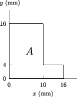
The Cartesian coordinate system xyz is chosen such that the axis z is parallel to the conductor under examination. The conductor cross section does not change along the conductor. The permeability of the conductor material is constant and is equal to the vacuum permeability 𝜇0, its resistivity does not depend on z, it is a function of x and y, 𝜚 = 𝜚(x, y). Figure 1 illustrates the cross section A of a conductor in the plane xy. The cross section is a rectangle with the sides w and h. Generally, A can be an arbitrary closed continuous set [17,18]. The same as its components, the external magnetic field
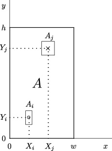
Cross section A of a conductor with marked cross sections A i and A j of two partial conductors.
By Faraday’s law of electromagnetic induction, the voltage U
ind is induced along an arbitrary closed continuous curve C, which lies in a magnetic field
The (not only rectangular) cross section A of a real conductor is a Jordan measurable set [17,18] and therefore any solid conductor can with arbitrary precision be replaced by partial conductors of rectangular cross section A
i
, ∀i (notation ∀i will be used instead of writing i = 1,2…, N). Let there be
In the paper the sets A i are assumed to be rectangles but they can also have a different shape; in [19], for example, they are sectors of circular ring.
Consider a segment of the conductor examined between the planes z = z
1 and z = z
2, z
2 > z
1. Together with z
1 and z
2, the points (X
i
, Y
i
) and (X
j
, Y
j
) (see Fig. 1) determine the loop C
ij
, which is formed by four line segments formed by the points (x, y, z):
Voltage is induced in the loop C
ij
according to formula (1), in which
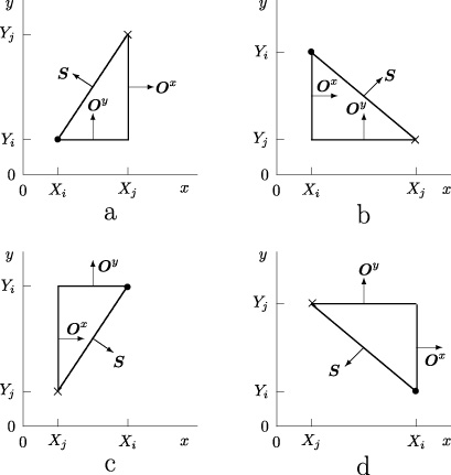
The points (X i , Y i ), ∀i, can be regarded as the vertices of the graph G. The edge in G between the vertices (X i , Y i ) and (X j , Y j ), i ≠ j, edge ij for short, is an intersection of the rectangle S ij with the plane z = 0 and in G it represents the loop C ij . Between the vertices (X i , Y i ) and (X j , Y j ) in G there is thus just one edge, the line segment joining the two vertices. The graph G is undirected because the loop C ij is the same as the loop C ji . No current is induced in the loops C ii , ∀i, and therefore it is no use considering the edges ii; G is thus a simple graph. Any two different partial conductors can form a loop and G can thus be a complete graph with K N = N (N −1)∕2 edges ij, ∀i, j; i ≠ j, [21]. For N > 3 it holds K N > N and some of loops are therefore dependent on the other loops. A dependent loop can be formed by the composition of independent loops. A dependent loop together with the loops it depends on will in G show as a closed path, which is a consequence of the magnetic field being solenoidal. In the graph G with the above properties there is a subgraph G tree, which has N vertices, N −1 edges, and does not contain any closed path of the graph G [21]. The edges of the subgraph G tree have their correspondent independent loops in the conductor examined.
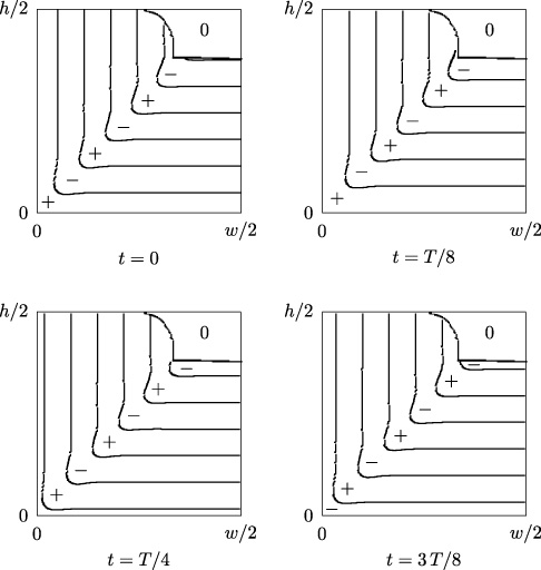
Figure 2 gives four examples of choosing a subgraph G tree ⊂ G in the cross section of a conductor subdivided into partial conductors of equally large rectangular cross sections. It follows from Fig. 2 that there can exist several subgraphs G tree that have the same vertices and differ in the position of the edges. However, the existence of at least one subgraph G tree ensures that there exist N −1 independent loops for N partial conductors. The formally simplest is the selection on the assumption that G tree is a path graph with the end-vertices (X 1, Y 1) and (X N , Y N ). The graph in Fig. 2a is not a path graph, in contrast to the remaining graphs in Fig. 2.

Conductor cross section A = [0,
Further in the exposition it is assumed that the graph G
tree is a path graph, i.e. the index j is equal to i +1. The index j, if it is together with the index i, can thus be omitted. The loop currents method can be applied to N −1 independent loops in the path graph. In Fig. 3 is a lumped-elements circuit which replaces the ith loop ∀i, i < N. In Fig. 3 there is also loop current in the (i −1)th and (i +1)th loops and current in the ith and (i +1)th partial conductors. Applying Kirchhoff’s voltage law to the circuit in Fig. 3 will yield the equation
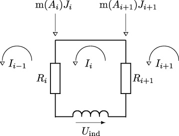
Replacement of the ith loop by a lumped-elements circuit, and loop currents in the (i −1)th and (i +1)th loops.
The flux
The proposed method for calculating the current density in a passive conductor is described by a system of Eqs (10) and (11). The application of the method will be demonstrated via solving several problems in both the steady state and the transient state.
Without loss of generality, it will be assumed that all the partial conductors are of the same rectangular cross section, i.e. m(A
i
) = m (A
j
), ∀i, j. The cross sections of the partial conductors form in the rectangular cross section of the conductor n layers in the direction of the axis y, with each layer containing m cross sections of the partial conductors. Let there be Δx =
The calculated current density J
i
, ∀i, is constant in the cross section of the ith partial conductor and is thus piecewise constant, which is an approximation of the real state. The calculation result is the more precise, the larger the value of N. In the Figures given below, the discontinuous values of the amplitude
In addition to the current density, the Joule dissipation power is also determined. The total current passing through the passive conductor is zero. In one part of the cross section the current is positive while in the rest of the cross section the current is negative. The two currents are of the same magnitude but opposite sign.
Sinusoidal field
B
ex
Of considerable significance among the possible dependence relations between the field
It follows from the above that the system of Eqs (10) and (11) can be solved in the complex domain if the complex external field and current density
If
The left side of equation (13) can, after being multiplied by the term ΔxΔy, be replaced by the sum of two complex numbers,
The time of current density calculation depends on the magnitude of N, where N = m × n for a conductor of rectangular cross section. The criterion for the choice of an appropriate magnitude N is generally the stabilization of the current density norm as a piecewise constant function on the conductor cross section or the norm stabilization of the vector 〈|
The dimensions of the cross section of the Cu conductor are
Figure 4 illustrates the current density phasor from Example 1. In Fig. 4 the curves for y = 0.1 mm and y = 7.9 mm are identical to the curves for y = 15.9 mm and y = 8.1 mm, respectively. The cause of the symmetry of the current density amplitude is the symmetry of the external field and of the conductor cross section with respect to the straight line y = 8 mm. The external field and the conductor cross section are also symmetrical with respect to the straight line x = 5 mm. Symmetrical with respect to this straight line is also the amplitude
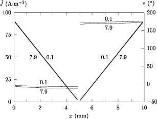
Dependence of the current density phasor on x for a constant y in Example 1. The thick lines give the amplitude
The conductor cross section dimensions are ten times the dimensions in Example 1,

Dependence of the current density phasor on x for a constant y in Example 2. The thick lines give the amplitude
The conductor resistivity is not constant. The conductor cross section dimensions are the same as in Example 1. The conductor is composed of m layers that are parallel to the plane yz. The cross section of the ℓth layer is the rectangle
The resistivity is not symmetrical with respect to the straight line x =
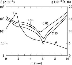
Dependence of the current density amplitude

Dependence of the initial phase ϵ of the current density on x for a constant y in Example 3. The numbers at the curves are the values of y expressed in mm.
The dimensions of the Al conductor cross section are
The external field, conductor cross section and resistivity are symmetrical with respect to the symmetry centre (
Dependence of the current density amplitude on x for a constant y in Example 4. The numbers at the curves are the values of y expressed in mm.
Regions of the zero current density amplitude in the conductor cross section in Example 4. Region 1: Al conductor, f = 106 Hz,
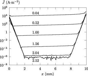
The dimensions of the Cu conductor cross section are
The external field, conductor cross section and resistivity are symmetrical with respect to the straight lines y =
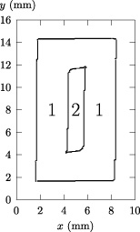
Regions in the left bottom quarter of the conductor cross section in Example 5, in which the current density J (x, y) has the same sign. In the region marked with the numeral 0 the current density is of negligible magnitude
The conductor cross section A is non-symmetrical, its shape and dimensions are given in Fig. 11. At a temperature of 25 °C the Al conductor resistivity is 𝜚 = 2.709 ×10⁻⁸ Ω ⋅ m [22], which does not depend on x and y. The field
Conductor cross section A in Example 6.
Figures 12 and 13 give the dependence of the current density phasor on x on the straight lines y = const. The partial conductors are of square cross section with the side Δx = 0.1 mm.

Dependence of the current density amplitude on x for a constant y in Example 6. The numbers at the curves are the values of y expressed in mm. The curves for y = 4.05 mm and y = 6.05 mm are dotted.
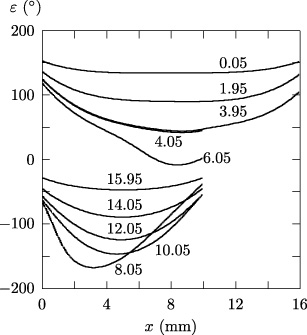
Dependence of the initial current density phase on x for a constant y in Example 6. The numbers at the curves are the values of y expressed in mm. The curve for y = 4.05 mm almost merges with the curve for y = 3.95 mm.
The dimensions of the Al conductor cross section are
An equation for the calculation of the current density in a conductor which is in the external field produced by a current filament that is parallel to the conductor and passes through the point (x
f
, y
f
) is obtained by substituting for
The current density phasor in Example 7 is illustrated in Figs 14 and 15.
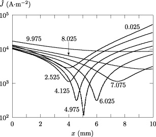
Dependence of the current density amplitude on x for a constant y in Example 7. The numbers at the curves are the values of y expressed in mm.
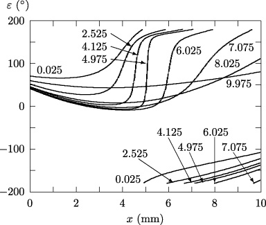
Dependence of the initial current density phase on x for a constant y in Example 7. The numbers at the curves are the values of y expressed in mm.
In the transition of the external field
As has been assumed, the partial conductor cross sections are identical and equation (11) can thus be replaced by the equation
Multiplying equation (19) by the inverse matrix
The positive current in the transient state depends on N and t
This example concerns switching on and off the external field with the components
The period of the field
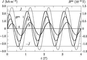
Dependence of the transient current density on time in four partial conductors, whose cross sections are cut by the diagonal of the conductor cross section in Example 8; the cross section centres of partial conductors are for curve 1: (9.95, 0.05) mm, 2: (9.35, 1.05) mm, 3: (8.35, 2.65) mm, 4: (5.05, 7.95) mm. The external magnetic field has a period T and its time dependence is illustrated by the thin line. The steady-state amplitude
Figure 17 gives the dependence of the global quantities I
+ and P on t in Example 8. The dotted line segment represents the value |
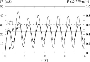
Dependence of I
+ (thick line) and P (thin line) on t in Example 8. The dotted line gives the value |
In Fig. 16 the dependence is given of the transient current density on t from the instant t = 0 (switching the external field on), when the external field passes through zero because its initial phase is zero. Figure 18 gives the dependence of the transient current density in partial conductors 1, 2, and 3 (see the caption to Fig. 16) when switching on at the instant t = 0 and when switching off at times t = 2.25 T and t = 2.4 T. The external magnetic field differs from the field specified in Example 8 in that its non-zero initial phase is 45°.
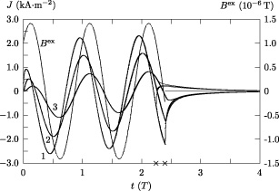
Dependence of the transient current density in partial conductors 1, 2, and 3 (see the caption to Fig. 16) when switching on at time t = 0 and off at times t = 2.25 T and t = 2.4 T. The dependence B ex(t) is shown as a thin line.
When solving some of the examples, the symmetry of the current density was mentioned. This symmetry is a consequence of the symmetry of the conductor cross section, external field and resistivity. Symmetry can be made use of when constructing the system of equations (10), (11) and to reduce their number to a half or quarter since due to the symmetry the number of unknown current densities gets lower. The time necessary to solve the system of equations (10), (11) is directly proportional to the third power of the number of equations; reducing their number can significantly reduce the calculation time, in particular when calculating the steady current density and when the values of m and n are high.
Various possible mutual positions of the points (X
i
, Y
i
) −
All the areas through which the relevant fluxes of the magnetic field vector flow lie inside the conductor examined and are thus affected by the magnetic properties of the conductor material. In the paper it is assumed that the conductor permeability is equal to the vacuum permeability 𝜇0. The vacuum permeability is sufficiently exact for diamagnetic and paramagnetic materials as well as for ferromagnetic materials at temperatures higher than their Curie temperature. In a linear material it holds
In equations (10) and (11) and in all the Examples the flux
In Example 7, the external field is produced by a single current filament. The external field flux is determined by relation (15), in which the dependence on t is given by the function I f(t). Similar to the preceding paragraph, the external field can be formed by a finite number of current filaments with different dependence relations I f(t).
On the assumptions as given in the Introduction section, the method for calculating current density in a passive conductor placed in time-variable magnetic field was exactly derived in a physically clear way. The derivation of the method is based on Faraday’s law of electromagnetic induction and is an application of the Biot and Savart law, the loop current method, Kirchhoff’s voltage law, Ohm’s law, the Jordan measure theory, and graph theory. These starting points cannot be called in question, the same as the result that follows from them. Current density is generally the solution of a system of equations formed by one algebraic equation (11) and N −1 ordinary differential equations of the first order (10). These equations allow calculating the current density in both the transient and the steady state. The numerical calculation is performed in two parts. The first part consists of calculating the equation coefficients, using the formulae given in the paper. The second part depends on whether the steady or the transient state is being solved. In the steady state the external field is sinusoidal and what is solved is a system of linear algebraic equations (12) and (13) in the complex domain. In the transient state the external field is of arbitrary given course and what is solved is a system of ordinary linear differential equations of the first order with initial conditions (20), using one of the known methods, e.g. the Runge–Kutta method [18,23].
The source of electromagnetic field is the electric charge. In the paper this field is a quasi-stationary magnetic field produced by a moving electric charge. The result of calculating by the proposed method is the current density. The current density directly determines the magnetic field [24] and Joule’s dissipated power.
The calculation of induced currents has been the subject of many publications. The methods proposed in these papers are based on Maxwell’s equations in differential form. By means of these equations, a partial differential equation of the second order is derived whose solution is the vector potential
In comparison with the published methods, the method for solving the problem as formulated in the Introduction section is general (it includes both the steady and the transient state). It does not require the knowledge of boundary conditions while the numerical calculation is very simple.
Conclusion
A simple method has been proposed for calculating the current density in a long solid conductor of arbitrary cross section which is not connected to a source and occurs in an external magnetic field. It is assumed that the external magnetic field is quasi-stationary and is unaffected by the magnetic fields of the currents induced in the conductor under examination. The frequency of the external field does not exceed 1 MHz and the displacement current is neglected. The permeability of the conductor material is constant and is equal to the vacuum permeability 𝜇0.
The essence of the proposed method consists in the conductor being replaced by N partial conductors of rectangular cross section and constant current density. The derivation of the method is based, in the first place, on Faraday’s law of electromagnetic induction and is an application of the Biot and Savart law, loop current method, Kirchhoff’s voltage law, Ohm’s law, the Jordan measure theory, and graph theory. The current density is generally the solution of a system of equations formed by one algebraic equation (11) and N −1 ordinary differential equations of the first order (10).
The application of the proposed method is demonstrated via solving eight examples. Results are given of the calculation of the current density in a conductor with symmetrical and non-symmetrical cross section, with constant and non-constant resistivity in the conductor cross section, for homogeneous and non-homogeneous external steady sinusoidal field, and for the case of switching the external sinusoidal field on and off.
Footnotes
Acknowledgements
This research work has been carried out in the Centre for Research and Utilization of Renewable Energy (CVVOZE). Authors gratefully acknowledge financial support from the Ministry of Education, Youth and Sports of the Czech Republic under OP VVV Programme (project No. CZ.02.1.01/0.0/0.0/16_013/0001638 CVVOZE Power Laboratories-Modernization of Research Infrastructure).
Appendix
According to formulae (8) and (9) the fluxes
The magnetic field
The flux through the rectangle S is determined by means of the fluxes of the vector
For the fluxes 𝜙(O
x
) and 𝜙(O
y
) of the vector
The flux 𝜙(S) of the vector
It follows from relation (9) that for a given function
The current filament which produces the external field is parallel to the axis z and passes through the point (x
f, y
f) in the plane xy. The current filament must lie outside the conductor examined and thus it cannot pass through the point (0,0). The magnetic field of the current filament at the point (x, y) can be calculated using Ampere’s circuital law; it holds
The flux