Quantitative control of the zero-bias-current electromagnetic bearings for lower power consumption

Abstract

Based on the non-contact characteristics, active magnetic bearings (AMBs) possess great benefits like no lubrication, high speed, high accuracy and long lifespan. Moreover, the rotor dynamic performance is adjustable and working conditions are monitorable. Nonetheless, AMBs suffer from large power loss and rotor heating. One viable approach is omitting the bias current, i.e., zero-bias AMBs, but this also results in high non-linearity and poor controllability. The common control practices of zero-bias AMBs are based on nonlinear models, for there is only one electromagnet being electrified at any moment to produce a net control force. In this study, we propose a linear control strategy for the zero-bias AMB. Assuming that each coil has an average current proportional to the pulse width modulation (PWM) duty cycle, the quantitative relation among the magnetic force, the rotor displacement and the coil current can be acquired. Further, this control algorithm was applied to both the horizontal and the vertical thrust zero-bias AMBs. Experimental results proved the existence of currents in both electromagnetic bearings in the unbalanced state. And the rotor-bearing system restored rapidly to an equilibrium state after sudden disturbances. Overall, this method demonstrates the transition from physics to engineering and shows a good application prospect.

Keywords

Zero-bias magnetic bearing mathematical model quantitative control PWM power consumption

1. Introduction

An active magnetic bearing (AMB) is a supporting part which uses variable electromagnetic forces to levitate a rotor; therefore, there are no contact and wear. High speed, high accuracy, no lubrication, free contamination etc. makes AMBs applicable for harsh working conditions, such as extreme temperature, extreme cleanliness and corrosive working fluids, where conventional lubricated bearings can’t function well [1–5]. Moreover, AMBs enable adjusting of dynamic motions of the system during operation and provide a valuable system control feature during regular operation [6,7]. As well known, the AMB system is open-loop unstable and highly nonlinear, consequently, requires continuous active control to guarantee stability [8]. The conventional way to deal with the AMB system is by adopting the Taylor series expansion to realize the linearization [9]. Nevertheless, the linearization loses efficacy without a constant bias current or bias flux. In fact, large bias current/flux is employed to achieve greater linearity and dynamic performance, whereas it brings about huge copper losses at the same time and reduces the running time of the AMBs [10]. Meanwhile, a bias current/flux also causes rotor heating [11], which impacts the operation at low temperature applications, such as in cryogenic turbo expanders. Therefore, various strategies [12–19] on diminishing power losses have been developed. These reports cover the innovations in mechanical structure, permanent magnets and variable bias current/flux. Each method possesses both relative merits and drawbacks. Take the permanent magnetic bearings for example, which decrease power consumption, yet increase the complexity in installation and extra cost. As a result, zero-bias current/flux control is proposed to minimize the power loss [20].

Zero-bias AMBs effectively eliminate the undesirable overheating, useless eddy current losses, hysteresis losses and Ohmic losses generated by the bias current/flux. They are expected in applications like cryogenic turbo expanders, aero-generators, artificial heart pump impellers, magnetic levitation display stands, craft gifts, etc. Even though zero-bias AMBs have lower stiffness, they are suitable for light-load situations or axial AMBs. For example, in the flywheel energy storage systems, large load capacity is not required, yet the bearing loss is necessary to be reduced to maintain the storage of energy for several hours. In fact, the problem is that the conventional way to linearize the AMB system can no longer work with the zero-bias, thus many nonlinear control laws have been employed on the zero-bias AMBs. Tsiotras et al. [21] investigated the stabilization of a zero-bias AMB by employing control Lyapunov functions. Charara et al. [22] proved the superiority of nonlinear control (without bias currents) over linear control (with bias currents) in the diminution of energy consumption; further, they proposed a sliding mode control strategy. Aside from that, advanced control like optimal control [11], H∞ control [23], and adaptive control [24] were studied for the zero-bias AMB system. Kato et al. [25,26] combined the self-sensing technique with a one-degree-of-freedom (1-DOF) zero-bias-current AMB, in which the rotor position is detected by carrier signals transmitted by a series resonance circuit inserted between the windings of the electromagnets. Tsiotras and Wilson [27] established a flux-based model which is effective for both zero- and nonzero-bias AMBs, and they also focused on the mitigation of the singularity problem. The drawback of zero-bias operation stems from the fact that the slope of the force curve at the origin is zero. This implies that to generate a small control force, a huge change in flux is necessary, which results in large voltage commands and potential voltage saturation on the condition of voltage-controlled designs [28,29]. Generally, there are several methods to tackle the singularity problem: permanent magnetic bearings, small current/flux bias [27], and cascaded systems [30]. Using permanent magnets to generate bias magnetic field can reduce the power loss and decrease rotor heating, but yet the structure is too complicated and is susceptible to demagnetization. Besides, the hysteresis and eddy current loss of the rotor cannot be cut down [31]. As for the cascaded position-flux control system, which enables operation at a zero bias and within the magnetic saturation, it brings much difficulty in the implementation of the inner loop flux observers. In [32], a variable force bias was introduced instead of a bias current to compensate for the nonlinearities. In [30,33], position-flux controllers based on flux control for zero-bias operation were explored. Despite these researches, zero-bias flux-controlled technology is scarcely feasible and is not common in industrial implementations, for flux is hard to be measured in practice. Although adopting a flux control enables reduced force estimation error and a better controller bandwidth than a classical current controller, flux sensors increase hardware complication and enlarge the air gap, which not only cause problematic integration in the AMBs, but also decrease the achievable bearing capacity [30].

Apart from nonlinear control strategies, linear control is also applicable to zero-bias AMBs, mainly the PID control. Linear control algorithms have a low computation intensity, which makes an easier implementation in practical applications [34]. Whereas, tuning parameters is rather tedious and time-consuming; moreover, system instability may possibly occur during parameters tuning, for the control parameters directly affect the bearing stiffness and damping [35]. Therefore, it is a good way to establish the mathematical model of zero-bias AMB system and figure out a rough range of parameters before fine tuning on the test rig.

As far as the authors are concerned, there are many researches on linear control of AMB systems [36–40], but few reports about linear control of zero-bias AMBs. The main reason is that previous researches following the rule that only one in a pair of coils is driven and has current flow at any time. In fact, the currents of both coils at any moment of the unstable condition may not be zero. The reason is that the frequency of the pulse width modulation (PWM) wave outputted from the controller can reach scores of kilohertz while the response of coil current has a lag due to the coil inductance. Even though the control signal electrifies only one coil at any time, the currents of both electromagnets could not be totally zero and are related to the PWM wave in a cycle of the control signal. Accordingly, in this paper, we propose the average-current concept. Assume that each coil has a current flow in every PWM period, and the magnitudes of the currents are relative to the duty ratio of the PWM wave. Based on this, the force analysis of the zero-bias AMB could be obtained. Regarding the balanced rotor-bearing system as a spring-oscillator system, the quantitative relation among the magnetic force, the rotor displacement and the coil current can be acquired by math modeling. Furthermore, possible values of control parameters are figured out and applied in the experiments.

This paper proceeds as follows. A review of previous work on zero-bias active magnetic bearings is presented in the introduction. The modelling of AMB with a bias current is presented in Section 2. Section 3 is about linear quantitative control of zero-bias AMBs with average current assumption, and both the horizontal and vertical thrust bearings are analyzed. Experimental setup is described in Section 4, following with experimental results of both the horizontal and vertical thrust bearings, then the calculation of power consumption, and discussions at the last. Finally, conclusions are drawn in Section 5.

2. Problem formulation

As illustrated in Fig. 1, the 1-DOF test rig comprises two electromagnets (EMs), a rotor disc suspending between the EMs, a displacement sensor resting aside the rotor, a controller connected to the sensor and power amplifiers (For detailed information on geometric parameters of the test rig, please refer to Table 1). Assuming that the rotor deviates from the equilibrium position by a perturbation, the displacement sensor detects the rotor position and transfers analog signals to the controller. After AD conversion and filter processing, the controller calculates the control value and then outputs digital control signals (i.e., PWM waves). Driven by the control signals, the switching power amplifiers output control currents to drive the EM. In this way, the rotor is dragged back to the equilibrium position rather than adhered to any EM as a result of shrinking air gap and enhanced attractive magnetic force.

Fig. 1.

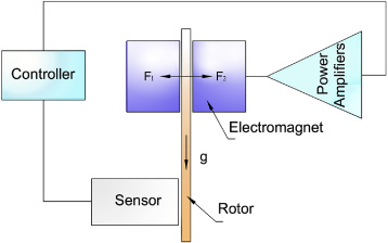
Schematic diagram of a 1-DOF AMB system.

Table 1

Test rig physical parameters

Nominal air gap	x ₀ = 0.585 mm	Maximum air gap	X ₀ = 1.17 mm
Rotor radius	r = 30 mm	Rotor width	w = 2.5 mm
Rotor mass	m = 60 g	Rotor material	Electrical iron
Nominal voltage	V = 24 v	Pole area of EM	S = 46.2 mm²
Coil turns (per coil)	N = 1884	Coil resistance	R = 180 Ω
Coil inductance	L = 12.9 mH	Peak force	f = 24.5 N

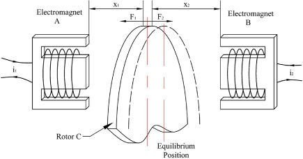
As shown in Fig. 2, the simplified 1-DOF zero-bias AMB model consists of two identical EMs, which generate attractive forces (F ₁ or F ₂) on the rotor. As well known, the magnetic force generated on the AMB is relative to the coil current and the air gap between the rotor and the stator, as given in the following equations [41] $\begin{eqnarray}\displaystyle F=ki^{2}/x^{2}, & & \displaystyle\end{eqnarray}$ (1) where i represents the coil current and x denotes the air gap between the rotor and the stator. k represents the magnetic force coefficient, which is related to the area of the electromagnet pole S and number of coil turns N (i.e., k = 𝜇₀ SN ²∕4).

Fig. 2.

Simplified model of the 1-DOF zero-bias AMB.

When the rotor deviates away from the equilibrium position, a control current is generated based on the rotor position. To gain a linear model, a constant current I ₀ is introduced to all the coils of the AMB [17]. Thus, the coil current is composed of a bias current I ₀ and a control current i _c. The total magnetic forces exerted on the rotor is $\begin{eqnarray}\displaystyle \displaystyle F_{1}-F_{2}=k\left[{\displaystyle \frac{(I_{0}-i_{c})^{2}}{(x_{0}-x_{u})^{2}}}-{\displaystyle \frac{(I_{0}+i_{c})^{2}}{(x_{0}+x_{u})^{2}}}\right], & & \displaystyle\end{eqnarray}$ (2) where x ₀ represents the nominal air gap and x _u denotes the rotor’s deviation from the equilibrium position. Suppose that x _u ≤ x ₀ and i _c ≤ I ₀, Eq. (2) can be simplified at the equilibrium point x ₀ using Taylor series expansion, which is written as $\begin{eqnarray}\displaystyle F_{1}-F_{2}=k_{i}i_{c}+k_{x}x_{u}, & & \displaystyle\end{eqnarray}$ (3) where $k_{i}=4kI_{0}/x_{0}^{2}$ is the current stiffness and $k_{x}=4kI_{0}^{2}/x_{0}^{3}$ is the displacement stiffness. Therefore, the control current can be obtained with a linear control law. The main advantage of the bias current is the linearization of the nonlinear AMB model. Nonetheless, the constant bias current also leads to much larger energy consumption and reduces the running time of the AMB. Besides, rotor heating is also brought about by a bias current, which impedes the application of AMBs in operations at low temperatures, such as in cryogenic turbo expanders.

Accordingly, the zero-bias AMB was proposed by researchers. Compared with the bias-current type, there is only one control input which is effective at any time depending on the rotor position. To realize the nonlinear control of the 1-DOF AMB, the control currents of the EMs are switched according to the rotor position (Fig. 3). As shown in Fig. 2, when the rotor deviates away from the equilibrium position, the switching power amplifier of the EM with shrinking air gap turns off while that of the EM on the opposite switches on to pull the rotor back. The switching process lasts until the rotor is back to the equilibrium position and almost stabilized. The total force on the rotor F is $\begin{eqnarray}\displaystyle F=\left\{\begin{array}{@{}ll@{}}f_{1}=ki_{1}^{2}/(x_{0}-x_{u})^{2} & (i_{1}\neq 0,i_{2}=0)\\[0.5pc] f_{2}=ki_{2}^{2}/(x_{0}+x_{u})^{2} & (i_{1}=0,i_{2}\neq 0),\end{array}\right. & & \displaystyle\end{eqnarray}$ (4) where i ₁ and i ₂ are the EMs’ currents. From Eq. ((4)), the relationship between the magnetic force and coil current is nonlinear. However, the nonlinear model is more complicated than a linear model. Hence, a new method to identify the linear relation among the magnetic force, the rotor displacement and control current of the zero-bias AMB is proposed in the following section.

Fig. 3.

Block diagram of zero-bias current AMBs.

3. Modeling of zero-bias AMBs with average current assumption

In this part, a mathematical model based on the average current assumption is established and quantitative control algorithm of zero-bias AMB is thereby calculated. Moreover, both the horizontal and the vertical thrust zero-bias AMBs are considered. The numerical model mainly describes the rotor motion. The total air gap between the EMs and the rotor is X ₀ (X ₀ = 2x ₀), of which x ₀ is the nominal air gap. To make it easier for programming, suppose that the air gap between EM A and the rotor is x, therefore the rotor displacement can be represented by (x ₀ − x). Both EMs are actuated by switching power amplifiers. Functioning as a gating signal to the switching power amplifiers, the PWM waves outputted from the controller are shunted into two signals, one of which remains the same, while the other is dealt with a negation operation through a NOT gate. Hence, the states of the two switching power amplifiers are mutually inverse. When PWM is at high level, one EM (suppose EM A) is electrified, and the other EM, i.e., EM B is not turned on. Therefore, the running time of the EMs are adjusted by the duty ratio of PWM. By this way, the control current of EM A is adjusted. In the modeling part, the maximal duty ratio of a PWM period is set to be 100, which is named the total current I ₀. If the duty ratio is 80, the control current of EM A in this PWM period is 0.8^∗ I ₀, and that of EM B is 0.2^∗ I ₀. Assuming that the average current of EM A is I (related to the output of the controller and also defined as control current), then that of EM B should be (I ₀ − I), which is different from common nonlinear control algorithms on the premise of only one EM being electrified at any time, namely the generalized complementary current condition (Fig. 4).

Fig. 4.

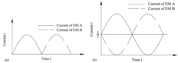
Coil currents of the zero-bias AMBs: (a) in complementary current condition with nonlinear control and (b) under average-current assumption with linear control.

3.1. Modeling of the horizontal thrust zero-bias AMB

From Eq. (1), the magnetic forces of the two EMs at a PWM period can be described as $\begin{eqnarray}\displaystyle F_{1}={\displaystyle \frac{kI^{2}}{x^{2}}}\quad F_{2}={\displaystyle \frac{k(I_{0}-I)^{2}}{(X_{0}-x)^{2}}}. & & \displaystyle\end{eqnarray}$ (5) When the rotor is disturbed and deviates from the equilibrium position, it is instantly dragged back by the varying magnetic resultant force in prevention of being tightly clung to the EM. Analogous to a classical spring damper system, the controller must provide a recovery force and damping to attenuate the oscillation, hence the resultant force has a functional relation with the rotor displacement and its velocity. Assume that the relation is linear. The total magnetic forces exerted on the rotor in this circumstance are: $\begin{eqnarray}\displaystyle \text{K}x_{u}+\text{D}\dot{x_{u}}=F_{1}-F_{2} & & \displaystyle\end{eqnarray}$ (6) $\begin{eqnarray}\displaystyle x_{u}=x-x_{0}, & & \displaystyle\end{eqnarray}$ (7) where K and D are constants named the displacement coefficient and the velocity coefficient, respectively. Substitute equations (5) and (7) into (6), leading to the following expression: $\begin{eqnarray}\displaystyle \text{K}(x-x_{0})+\text{D}{\displaystyle \frac{d(x-x_{0})}{dt}}={\displaystyle \frac{(I_{0}-I)^{2}}{(X_{0}-x)^{2}}}-{\displaystyle \frac{I^{2}}{x^{2}}}. & & \displaystyle\end{eqnarray}$ (8)

To solve Eq. (8) and establish a linear model among the control current I, rotor displacement x _u, and $\dot{x_{u}}$ , the coefficient K and D should be figured out. Since Eq. (8) cannot be solved immediately, a small simplification is made by omitting the damping effect (i.e., D = 0) at the initial step, thus the model of K, I and x could be figured out. Then an appropriate K value is chosen based on a larger linear relation range among K, I and x. An appropriate K value makes the control current I cover the whole air gap and the velocity term, to ensure the suitability of the algorithm in case of large rotor displacement and velocity. Next, reconsidering the damping effect in Eq. (8) by introducing a new velocity term Y and recalculate the equation with a specific K value. After that, a nonlinear model among control current I, velocity term Y and rotor position x can be figured out. Finally, after surface fitting, the linear relation among I, Y , x can be figured out with precise coefficients, which can be used as control parameters of a linear control law of the zero-bias AMB.

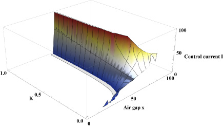
Specifically, the maximum duty ratio of the PWM is a constant. To make it clear while programming, the maximum duty ratio is set to be 100; hence, the total current of each PWM period (i.e., I ₀) can be divided into 100 parts. To simplify the algorithm, the total air gap X ₀ can be also discretized into 100 parts. Based on Eq. ((8)), the functional relation among displacement coefficient K, control current I and air gap x can be obtained by initially neglecting the velocity coefficient via Mathematica Software. As demonstrated in Fig. 5, when K varies from 0 to 1, the range of control current I is always [0, 100], however, that of the air gap shrinks from [0, 100] to [40, 60] with an increasing K value. Furthermore, to calculate Eq. ((8)), a new variable Y is introduced, which contains the change of rotor velocity, thus named the velocity term. 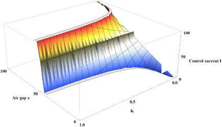$\begin{eqnarray}\displaystyle Y={\beta}\dot{x_{u}}. & & \displaystyle\end{eqnarray}$ (9) In Eq. ((9)), 𝛽 is a coefficient. Accordingly, Eq. ((8)) can be resolved with a constant K. Based on Fig. 5, the appropriate value of K is around 0.5; hence, different K values from 0.03 to 0.055 are calculated to demonstrate the impact on control current I, rotor position x, and velocity term Y . As shown in Fig. 6, when K = 0. 03–0.035, the control current reaches saturation in case of large air gap or velocity term. On the contrary, when K = 0. 045–0.055, the control current is not large enough to cover the whole air gap. Hence, the appropriate value of K should be 0.04.

Fig. 5.

Functional relation among displacement coefficient K, control current I and air gap x (horizontal direction).

Fig. 6.

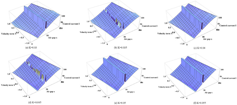
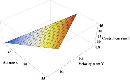
Functional relation among control current I, air gap x and velocity term Y with different K values (horizontal direction).

When K = 0. 04, the equation roots of Eq. (8) are listed as follows: $\begin{eqnarray}\displaystyle \begin{array}{@{}l@{}}I_{1}={\displaystyle \frac{0.01(50x^{2}+1.414\sqrt{\triangle })}{-50+x}}\qquad I_{2}={\displaystyle \frac{0.01(50x^{2}-1.414\sqrt{\triangle })}{-50+x}}\\[12.0pt] \triangle =-1.25\times 10^{7}x^{2}+1.25\times 10^{6}x^{3}-31250x^{4}+300x^{5}\\[12.0pt] \qquad -x^{6}+1.25\times 10^{7}x^{2}Y-5\times 10^{5}x^{3}Y+6250x^{4}Y-25x^{5}Y.\end{array} & & \displaystyle\end{eqnarray}$ (10)

Hence, the functional relation among control current I, air gap x and the velocity term Y has been figured out (Eq. (10)), still the formulas are needed to reduce order. The equation roots can be plotted via Mathematica software (Fig. 7), and we can conclude that only the second equation root (b) is reasonable. Figure 7b can be fitted as a planar to simplify the high degree polynomial among I, x, and Y. Thus, the fitting surface is obtained through several scattered points (Fig. 8). The analytic expression of Fig. 8 is listed in the following, which can also be used as the algorithm of control output. 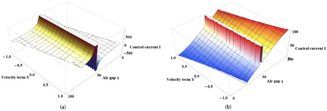$\begin{eqnarray}\displaystyle I=K_{P}x_{u}-K_{D}\dot{x_{u}}+C, & & \displaystyle\end{eqnarray}$ (11) where K _P = 1.8 and K _D = −0.3 are defined as recovery coefficient and damping coefficient, respectively. C is a constant. Equation ((11)) indicates a current-control algorithm. According to the rotor’s dynamic state (i.e., rotor’s deviation from the equilibrium position and the rotor’s velocity), the control current can be obtained. To prevent from magnetic saturation, the maximum current value of the zero-bias AMB system is assigned as 100 in case that the calculated control current from Eq. ((11)) value exceeds 100.

Fig. 7.

Roots of Eq. (10): (a) the first equation root and (b) the second equation root.

Fig. 8.

Linear functional relation among control current I, air gap x and the velocity term Y (horizontal direction).

3.2. Modeling of the vertical zero-bias thrust AMB

In this section, the theoretical calculation of the vertical zero-bias thrust AMB has been conducted. As known, the thrust magnetic bearing in the vertical direction needs to bear the rotor gravity. Compared with traditional AMBs, there is no bias current to support the rotor. Nevertheless, we can calculate the desired PWM ratio of the upper EM to bear rotor gravity. Then the rest PWM ratio can be allocated to both EMs according to the sudden unbalance with the average current assumption.

Firstly, the upper EM has a larger current ratio than the bottom EM to compensate for rotor gravity. For the upper EM: $\begin{eqnarray}\displaystyle F_{1}=kI_{c}^{2}/x_{0}^{2}=mg, & & \displaystyle\end{eqnarray}$ (12) where I _c is the compensating current of the upper EM. By this way, the compensation current portion can be calculated. And the remaining current portion is used to balance the rotor position. The total forces except the rotor gravity can be written as: $\begin{eqnarray}\displaystyle \textit{K}(x-x_{0})+\textit{D}{\displaystyle \frac{d(x-x_{0})}{dt}}={\displaystyle \frac{(I_{0}-I_{c}-I_{v})^{2}}{(X_{0}-x)^{2}}}-{\displaystyle \frac{I_{v}^{2}}{x^{2}}}, & & \displaystyle\end{eqnarray}$ (13) where I _v is the current of the bottom EM. The calculation process is the same as the horizontal bearing. As seen in Fig. 9, a smaller K value has a larger air gap. Hence, different K values from 0.018–0.04 are calculated to figure out the appropriate value. By introducing a damping term Y , the relation among control current I, air gap x, and velocity term Y can be figured out. As exhibited in Fig. 10, when K = 0.018−0.02, the control current reaches saturation in case of large air gap or velocity term. On the contrary, when K = 0.03−0.04, the control current is not large enough to cover the whole air gap. Hence, the appropriate value of K should be 0.025.

Fig. 9.

Functional relation among displacement coefficient K, control current I and air gap x (vertical direction).

Fig. 10.

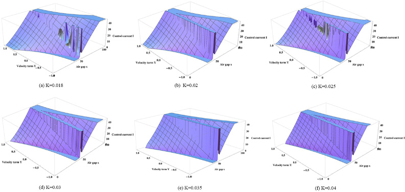
Functional relation among control current I, air gap x and velocity term Y with different K values (vertical direction).

When K = 0.025, the equation roots of Eq. ((13)) are listed as follows: $\begin{eqnarray}\displaystyle \begin{array}{@{}l@{}}I_{v1}={\displaystyle \frac{0.001(277x^{2}-\sqrt{\triangle })}{-50+x}}\qquad I_{v2}={\displaystyle \frac{0.001(277x^{2}+\sqrt{\triangle })}{-50+x}}\\[12.0pt] \triangle =-2.36\times 10^{9}x^{2}+1.72\times 10^{8}x^{3}-3.99\times 10^{6}x^{4}+37500x^{5}\\[12.0pt] \qquad -125x^{6}+2.5\times 10^{9}x^{2}Y-10^{8}x^{3}Y+1.25\times 10^{6}x^{4}Y-50000x^{5}Y.\end{array} & & \displaystyle\end{eqnarray}$ (14) Therefore, the functional relation among control current I, air gap x and the velocity term Y has been figured out (Eq. ((14))), still the formulas are needed to reduce the order. The equation roots can be plotted via Mathematica software and only the first equation root is reasonable, which can be fitted as a planar to simplify the high degree polynomial among I, x, and Y . Thus, the fitting surface is obtained through several scattered points (Fig. 11). The analytic expression of Fig. 11 can be obtained: $\begin{eqnarray}\displaystyle I_{v}=K_{P}x_{u}-K_{D}\dot{x_{u}}+C. & & \displaystyle\end{eqnarray}$ (15) Accordingly, the control current of the upper EM can be written as: $\begin{eqnarray}\displaystyle I=K_{P}x_{u}-K_{D}\dot{x_{u}}+C+I_{c}. & & \displaystyle\end{eqnarray}$ (16)

4. Experiments and analysis

In this section, the zero-bias electromagnetic bearing test rigs were set up, and three groups of experiments were carried out to testify the feasibility of the quantitative control algorithms. The first experiment was the calibration of electromagnetic forces and verification of the average-current assumption. Then, the quantitative control algorithm was applied to a horizontal zero-bias thrust AMB to test whether it could levitate the rotor successfully in case of sudden imbalance. After that, the vertical quantitative control algorithm was also applied to a vertical zero-bias thrust AMB in the same way. Finally, it was the experimental analysis.

Fig. 11.

Linear functional relation among control current I, air gap x and the velocity term Y (vertical direction).

4.1. Experiment setup

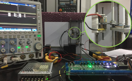
As seen in Fig. 12, two EMs, a rotor, a displacement sensor, a controller and two power amplifiers constitute the axial magnetic bearing test rig. The EMs are two small attracted-disk electromagnets with EI shaped cores, which are widely applied in auto equipment (experimental device, manipulator, cutting, grinding, sorting, etc.). The rotor is an iron disc with wall thickness 2.5 mm and diameter 60 mm. The displacement sensor (LANBAO LR18XBF05LIUM-4M) is eddy current type which outputs analog voltage within the range of 0–10 v, 1%FS. The digital controller discussed in this paper is implemented on K60 microprocessors (Freescale 32-bit), and the control program is designed with the IAR development environment. Two switching power amplifiers which mainly comprise MOSFET (IRF540N) are applied to drive the EMs. Table 1 details some of the physical parameters of the test rig.

Fig. 12.

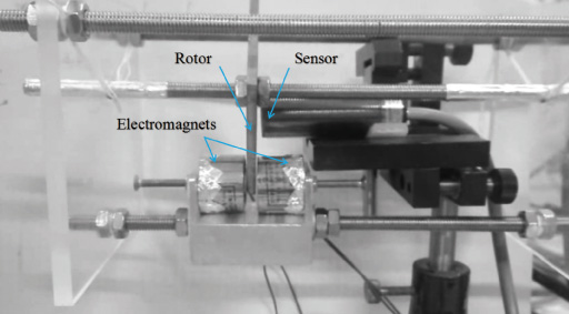
Picture of the axial zero-bias magnetic bearing test rig.

In particular, the AMB control system is a typical embedded system, which consists of four modules: the eddy sensor module, the K60 minimal system module, the power amplifier module and the power supply module. Specifically, the eddy current type sensor possesses high linearity and rapid response, which is essential to close-loop feedback control, for it reduces time delay and enhances the system response speed. The K60 minimal system module functions as the control center, including converting the sensor’s output voltage, processing digital signals based on the control algorithms, and driving the power amplifier module. The power amplifier modules drive the EMs in response of the control signals (i.e., PWM waves). In addition, the power supply module serves for the whole system’s hardware, including 5 v DC power supply for logical circuits, 3.3 v DC for the micro-controller, 24 v DC for both the eddy sensor module and power amplifiers.

The micro-controller K60 is the core of the embedded control system, of which the dominant frequency is 128 MHz. The Flash ROM is 512 KB, and the interfaces are common interfaces such as SPI, SCI, and IIC. Considering the high precision of the internal AD of the K60 micro-controller, the AD conversion circuit can be omitted by using the micro-controller’s own internal AD. The circuit design process should comply with reliability, efficiency and conciseness, of which reliability is the uppermost. One significant way to ensure system reliability is to separate the analog section and the digital section. Moreover, electromagnetic compatibility (EMC), shielding, grounding as well as filtering should all be taken into account.

The software design of the AMB system mainly contains 3 parts, i.e., under-layer software initialization, data acquisition & processing, and the control algorithm. The under-layer software initialization covers clock initialization, I/O port initialization, pulse wave initialization, interruption initialization, timer initialization, AD initialization, sensor and variable initialization. A function is written to let AD acquire the output voltages of the sensor. Suppression filter and interference cancellation are of essence in the prevention of inevitable noises and disturbance during data acquisition. Hence, weighting recursive averaging filtering is undertaken. Define a circular queue of which the length is N and each period a new sample value joins in at the tail of the queue till the total number of samples reaches N, then the head sample will dequeue and a new sample at the right moment enqueues. The more recently the sample data are, the larger weight coefficients they possess. This method is undertaken in AMB data-acquisition system due to its suitability for the realtime system and the convenience of changing sensibility by adjusting weight coefficients. The third part of the software design is the self-stabilizing control algorithm, which contains the initial calibration algorithm and the current control algorithm. The initial calibration algorithm aims to obtain the median value of the sensor output, which represents the balance position of the 1-DOF magnetic levitation test rig. The median value is acquired by electrifying the left electromagnet and the right electromagnet respectively; however, there should be some residual for correction.

PWM is a pulse wave of which the high level in each period is proportional to the transient analog signal. Applying PWM avoids digital-to-analog conversion (DAC) from the controller to electromagnets for the fact that digital signal is more immune to interferences. Additionally, digital signals can be implemented by an electronic switch (i.e., MOSFET) regardless of the mathematical model of the controlled object [42].

Based on PWM, a power amplifier circuit is designed (Fig. 13), which consists of a DC power supply (24 v), two NOT gates (SN74HC14N), two MOS tubes (IRF540N), two fly-wheel diodes (IN 5208), two LEDs and two divider resistances (5 k𝛺). IN 5208 is used to prevent the breakdown of IRF540N in case of a power failure and superimposed induced electromotive force. Two LEDs are parallel to the electromagnets to monitor the circuit’s working situation. When the digital output from the controller (i.e., the PWM wave) is at a high level, the contact point of the MOS tube is closed, and the circuit is in a power-on state, hence the electromagnet is electrified. Moreover, the PWM wave is shunted into two signals, one of which drives the MOS tube directly, while the other is initially tackled with a negation operation through a NOT gate. As a result, the two electromagnets have opposite working situations in each period.

Fig. 13.

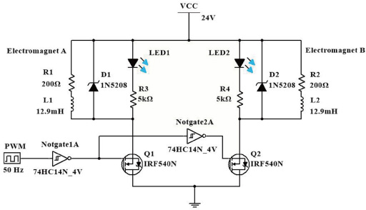
Schematic diagram of the switching power amplifiers.

4.2. Electromagnetic force calibration and average-current verification

Since the electromagnetic force has an important impact on the motion of the rotor, the electromagnetic force was calibrated experimentally (i.e., the calibration experiment). As demonstrated in Fig. 14, with the increase of the air gap, the electromagnetic force decayed rapidly. When the air gap exceeded 1 mm, the electromagnetic force became very weak. Therefore, to obtain an energy-efficient AMB system and make it easier for linear control, the air gap should be as small as possible. However, a very small air gap demands much higher control frequency and more expensive hardware system. Here, the nominal air gaps were designed to be 0.585 mm for the horizontal test rig and 0.5 mm for the vertical test rig, which were appropriate values in practice.

Fig. 14.

Calibration of the electromagnetic force.

After figuring out the appropriate air gaps of the magnetic bearings, the validation of the average-current assumption was conducted. The schematic circuit has been illustrated in Fig. 15, compared with the AMB system (see Fig. 1), two current probes have been added to the circuit. The current probe is an electric device with jaws which open to allow clamping around the electric coils. This allows measurement of the coil currents of the EMs without physical contact with it. In this test, two probes with an additional oscilloscope are applied to record the magnitude and waveforms of the alternating currents of two EMs in response to sudden disturbances.

Fig. 15.

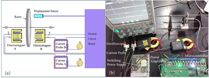
Validation of the average-current assumption: (a) the schematic circuit and (b) photograph of the detecting devices.

As shown in Fig. 16, when the rotor disc was initially at the equilibrium position or finally returned to a stable state, the coil currents in both EMs were nearly zero. Specifically, when there was a horizontal load with a direction towards EM B exerting on the rotor disc, the current of EM A increased immediately, while that of EM B remained zero. While the rotor was approaching EM B, the rotor velocity decreased, so was the control current of EM A. When the rotor reached the closest position to EM B, the rotor velocity was near zero. Since the electromagnetic force of EM B was very weak, the rotor quickly returned to the other side under the attractive force of EM A. To prevent adhesion to EM A, the control current of EM B increased to drag the rotor back to the equilibrium position, and the PWM duty ratio of EM A instantly decreased. Due to the self-inductance of EM A, the current in EM A changed from positive value abruptly to a negative value, instead of being zero. After the rotor reached steady state, the actual currents of both EMs are high frequency alternating currents, and are nearly zero when the system is stabilized. In addition, the rotor-bearing system resumed the equilibrium state with a very short period of time (approximately 1 ms), which proved the fast frequency of the PWM wave outputted from the controller. Moreover, the response of coil current has a lag due to the continuity of the coil inductance. As a result, even though the control signal electrifies only one EM coil at any moment, the currents of both EMs are not totally zero and related to the duty ratio of the PWM (i.e., the control signal). Based on the experimental results, the average-current assumption is reasonable.

Fig. 16.

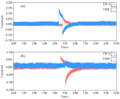
Coil currents of both EMs under sudden external loads exerting on the rotor disc: (a) a horizontal load towards EM B and (b) a horizontal load towards EM A.

4.3. Application to the horizontal zero-bias thrust AMB

The verification experiments were carried out to testify the feasibility of the quantitative control algorithm for the horizontal zero-bias thrust AMB. In this part, the rotor displacement under a disturbance were recorded via LabVIEW software. As illustrated in the previous statements, the maximal displacement of the disc had been discretized into 100 parts, and the initial equilibrium position was 50. Equation (11) implied that the control current was directly proportional to both the rotor’s offset from the equilibrium position and the rotor’s velocity, thus two groups of tests were performed. In practice, the duty ratio of the PWM wave was quantized into 1000 parts; therefore, the coefficients in Eq. (11) should be magnified 10-fold. The first group remained the damping coefficient K _D unchanged and varied the recovery coefficient K _P. As depicted in Fig. 17, when K _P = 18, the disc returned to the original equilibrium point within 3 ms after a step disturbance. As the recovery coefficient varied around the theoretical value, for example, K _P = 15 or 21, the system finally reached a steady state yet with a steady-state error.

Fig. 17.

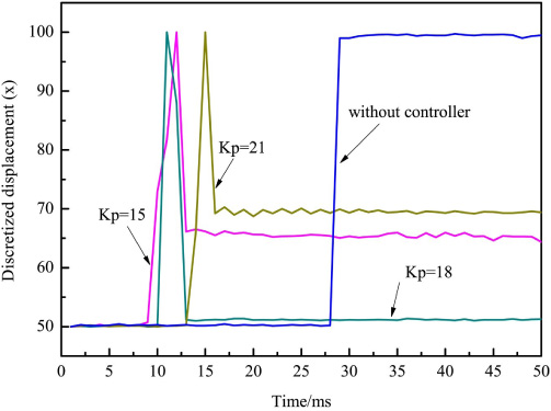
Performance of the axial zero-bias AMB system when the recovery coefficient K _P varied and the damping coefficient K _D remained unchanged in response of a disturbance.

With respect to the second group, the damping coefficient K _D became the control variable while the recovery coefficient K _P stayed the same. As seen in Fig. 18, the disc returned to the equilibrium point within 2.5 ms after a step disturbance. As K _D = −6, and resumed within 4.2 ms when K _D = −3, within 4.3 ms when K _D = 1. The graph manifested that as the magnitude of K _D increased negatively, both the relaxation time and the system steady-state errors were reduced. Furthermore, in Figs 17–18, the rotor displacements range from 49.977 to 100 (dimensionless displacement). Considering the symmetry properties of the system, this control algorithm is effective in 0 100, i.e., within the whole air gap. The experiments also recorded the dynamic performances of the system without a controller. As shown in Figs 17–18, the rotor without the controller was tightly clung to one EM after an external disturbance and could not return to the equilibrium position. The fact is that a shrinking air gap caused by the disturbance resulted in greater magnetic adhesion (Fig. 14).

Fig. 18.

Performance of the axial zero-bias AMB system when the damping coefficient K _D varied and the recovery coefficient K _P stayed the same under a disturbance.

4.4. Application to the vertical thrust zero-bias AMB

In this part, the quantitative control algorithm of the vertical direction was applied to a vertical thrust zero-bias AMB (Fig. 19). The coil currents of both EMs were detected by the current probes. Moreover, the rotor displacement was recorded by the data acquisition card.

Fig. 19.

Photograph of the vertical thrust zero-bias AMB.

As shown in Fig. 20a, vertical loads towards EM A were exerted on the system and the rotor initially moved toward EM A. However, the coil current of EM A decreased rapidly and consequently the rotor returned to the equilibrium position. In Fig. 20b, a vertical load towards EM B was exerted on the rotor, the coil current of EM A increased immediately; thus the rotor was dragged back to the balanced position. In addition, in Fig. 20, the range of rotor displacement from the equilibrium position to one EM side was 0.251 mm, which was half of the vertical air gap (0.5 mm). Figure 21 manifests the coil currents of both EMs within 60 ms at the steady state. The coil current of EM A was always higher than that of EM B to balance the weight of the rotor.

Fig. 20.

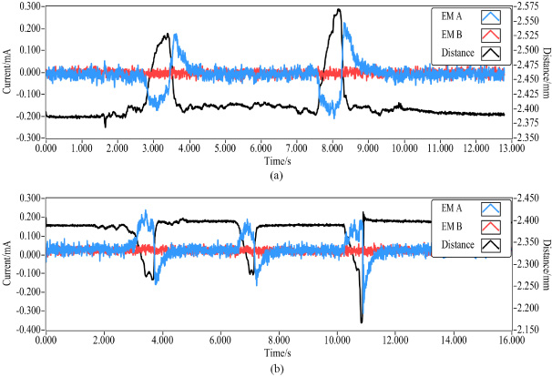
Coil currents of both EMs under sudden external loads exerting on the rotor disc: (a) a vertical load towards EM A and (b) a vertical load towards EM B.

Fig. 21.

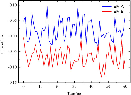
Coil currents of both EMs at steady state of the vertical thrust zero-bias AMB.

4.5. Power consumption

Power consumption of the pair electromagnets (i.e. EM A and EM B) can be computed by measuring the control currents over a period of time. If the coil resistance of the electromagnet is known, the electrical power consumption of the AMB is $\begin{eqnarray}\displaystyle P=(i_{1}^{2}+i_{2}^{2})R, & & \displaystyle\end{eqnarray}$ (17) where i ₁, i ₂ are the coil currents of both EMs and R is the coil resistance. This method does not contain the shaft power consumption (mainly the eddy current) since it is small compared with the electrical power losses of the AMB. For the AMBs with a bias current, the control current is treated as a constant which is one-tenth of the bias current.

For comparison, the power loss was measured under varied operating conditions for both zero-bias (ZB) and current-biased (CB) conditions. As shown in Table 2, in the steady state of the horizontal thrust AMB, the copper losses for ZB and CB (0.1 A) is about 0.012 w and 3.6 w, respectively. Meanwhile, the power losses of the vertical thrust AMB at steady state are 0.0026 w for ZB and 5.18 w for CB (0.12 A). Furthermore, the power consumption under external disturbance is also calculated. The copper losses for ZB and CB (0.1 A) are about 1.01 w and 4.36 w for the horizontal thrust AMB, and that of the vertical thrust AMB are 0.0136 w and 6.27 w, respectively.

Table 2

Power consumption of the AMBs without and with bias currents

	Horizontal thrust AMB		Vertical thrust AMB
	ZB	CB(0.1 A)	ZB	CB(0.12 A)
Stabilized condition	0.012 w	3.6 w	0.0026 w	5.18 w
External disturbance	1.01 w	4.36 w	0.0136 w	6.27 w

(*) ZB:zero-bias; CB: current-biased.

Compared with the current-biased AMB in case of external disturbance, the ZB operation decreases power loss by 76. 3% for the horizontal and 99.78% for the vertical. Meanwhile, the results also show that the power consumption converges to zero in absence of disturbance. Hence, the zero-bias current controlled methods decrease the power consumption of the AMB system tremendously, avoid the problem of over-heating caused by long-time running and provide a longer life for the AMB system.

4.6. Analysis of the experimental results

In all, the calibration experiment (Fig. 14) reveals strong non-linearity of the electromagnetic force and indicates an energy-efficient operating air gap roughly within 1 mm. As for the validation of the average-current assumption (Fig. 16), experimental results show that there are currents in both EMs during the unstable states, and possible analysis has been provided.

In respect of the verification of the quantitative control algorithm (Figs 17,18) of the horizontal zero-bias thrust AMB, the disturbed system soon returned to steady state in approximately 3 ms and was close to the previous state (with a fractional error ≤ 0.6%). Compared with the system without a controller, the control parameters around the theoretical value can reach the steady state. Further, the conclusion drawn from Fig. 18 manifests that a negative damping coefficient, which possesses a larger magnitude has better dynamic performance, which is slightly distinct from the theoretical calculation. The reason is that the velocity coefficient 𝛽 (Eq. (9)) is not covered in the damping coefficient K _D. Therefore, the damping coefficient requires fine tuning and small correction. In addition, Figs 17–18 manifest that slight steady-state errors ≤ 0.6% exist after disturbances, which is due to the simplification in the modeling process, such as omitting the nonlinear factors in the actual devices. Yet this control law can be improved by fine tuning the integral controller parameter, i.e., constant C in Eq. (11). In all, the feasibility of the modeling method itself is not affected.

As for the quantitative control of the vertical zero-bias thrust AMB, the result shows that the average-current assumption is also feasible as long as a proportion of PWM compensating for the gravity. Furthermore, from Figs. 17–18 and Fig. 20, the rotor displacements imply that the control algorithm is effective in 0--100, i.e., within the whole air gap. As for the rotor velocity, the maximal velocity is around the equilibrium position, when a sudden external load exerts on the rotor disc. However, the rotor quickly resumes the equilibrium position after sudden external loads. Therefore, the zero-bias control algorithm can apply to the motion of large displacement and velocity. The experimental results prove a high accuracy of the theoretical calculation, which also help avoid the tedious parameter-tuning process via trial and error.

5. Conclusions

This paper provides a new idea when dealing with the zero-bias AMBs and reduces the power consumption. The quantitative control algorithm sets up a linear model of the nonlinear zero-bias AMB system, which has a low computation intensity and easy implementation. This algorithm has been applied to a horizontal thrust bearing and a vertical thrust bearing, respectively. The main conclusions are as follows:

The average current assumption has been validated. Both EMs exit currents when the system is not stabilized. Moreover, the result also shows that the coil currents of both EMs are nearly zero in absence of disturbance.

Rotor levitation of the horizontal thrust zero-bias AMB has been achieved and appropriate stabilizing control parameters are figured out by mathematical calculation, which avoids a tedious parameter tuning process. Further, this algorithm also demonstrates good control performance and robustness in case of external disturbance. The system resumed to stabilization in approximately 3 ms and was close to the previous state (with a fractional error ≤ 0.6%).

This method can be generally used. With rotor gravity, this quantitative algorithm also realized rotor levitation of the vertical zero-bias thrust AMB, which resumed stability within 10 ms after sudden external loads (with a fractional error ≤ 0.8%).

The power consumption of the zero-bias thrust AMB with linear control are nearly zero at stabilizing conditions. That of the zero-bias thrust AMB in case of sudden external disturbance can be reduced by 76.3% (horizontal), 99.78% (vertical) compared with the current-biased AMB. The lower power consumption avoids the problem of over-heating caused by long-time running and provides a longer life for the AMB system.

Footnotes

Acknowledgements

The authors are grateful for the supports of the National Natural Science Foundation of China (grant no. 51276016) and China Scholarship Council (CSC).

References

Mushi

S.E.

Lin

and Allaire

P.E.

, Design, construction and modeling of a flexible rotor active magnetic bearing test rig, in: ASME Turbo Expo 2010: Power for Land, Sea, and Air, American Society of Mechanical Engineers, 2010, pp. 443–452.

Y.Y.

Lei

Sun

and Wang

, Effects of magnetic flux leakage of axial electromagnetic bearing on bearing system, International Journal of Applied Electromagetics and Mechanics 48(4) (2015), 357–366.

Y.Y.

Lei

Sun

and Wang

, Dynamics of magnetic suspension rotor system of turbo-expander, International Journal of Applied Electromagetics and Mechanics 54(1) (2017), 1–12.

R.Q.

Zhang

and Yao

M.H.

, Nonlinear dynamics near resonances of a rotor-active magnetic bearings system with 16-pole legs and time varying stiffness, Mechanical Systems and Signal Processing 100 (2018), 113–134.

Srinivas

R.S.

Tiwari

and Kannababu

, Application of active magnetic bearings in flexible rotordynamic systems–A state-of-the-art review, Mechanical Systems and Signal Processing 106 (2018), 537–572.

Halminen

Aceituno

J.F.

Escalona

J.L.

Sopanen

and Mikkola

, Models for dynamic analysis of backup ball bearings of an AMB-system, Mechanical Systems and Signal Processing 95 (2017), 324–344.

Neisi

Sikanen

Heikkinen

J.E.

and Sopanen

, Effect of off-sized balls on contact stresses in a touchdown bearing, Tribology International 120 (2018), 340–349.

Fonseca

C.A.

Santos

I.F.

and Weber

H.I.

, Experimental comparison of the nonlinear dynamic behavior of a rigid rotor interacting with two types of different radial backup bearings: Ball & pinned, Tribology International 119 (2018), 250–261.

Kameno

S.G.H.

, Application of zero-bias current active magnetic bearings to flywheel energy storage systems.

10.

Rong

and Zhou

, Nonlinear zero-bias current control for active magnetic bearing in power magnetically levitated spindle based on adaptive backstepping sliding mode approach, Proceedings of the Institution of Mechanical Engineers, Part C: Journal of Mechanical Engineering Science 231(20) (2017), 3753–3765.

11.

Yang

and Knospe

, Optimal control of a magnetic bearing without bias flux, in: American Control Conference, 1997. Proceedings of the 1997, Vol. 3, IEEE, 1997, pp. 1534–1538.

12.

Maslen

E.H.

Allaire

P.E.

Noh

M.D.

and Sortore

C.K.

, Magnetic bearing design for reduced power consumption, Journal of Tribology 118(4) (1996), 839–846.

13.

Fan

Y.H.

Lee

A.C.

Hsiao

F.Z.

, Design of a permanent/electromagnetic magnetic bearing-controlled rotor system, Journal of the Franklin Institute-Engineering and Applied Mathematics 334(3) (1997), 337–356.

14.

Sahinkaya

M.N.

and Hartavi

A.E.

, Variable bias current in magnetic bearings for energy optimization, IEEE Transactions on Magnetics 43(3) (2007), 1052–1060.

15.

Chen

S.Y.

and Song

M.H.

, Energy-saving variable bias current optimization for magnetic bearing using adaptive differential evolution, in: International Conference in Swarm Intelligence, Springer, 2017, pp. 466–474.

16.

Hsu

C.T.

and Chen

S.L.

, Nonlinear control of a 3-pole active magnetic bearing system, Automatica 39(2) (2003), 291–298.

17.

Chen

S.L.

and Hsu

C.T.

, Optimal design of a three-pole active magnetic bearing, IEEE Transactions on Magnetics 38(5) (2002), 3458–3466.

18.

Chen

S.L.

and Weng

C.C.

, Robust control of a voltage-controlled three-pole active magnetic bearing system, IEEE/ASME Transactions on Mechatronics 15(3) (2010), 381–388.

19.

Bassani

, Levitation of passive magnetic bearings and systems, Tribology International 39(9) (2006), 963–970.

20.

Basovich

Arogeti

and Brand

, Adaptive output zero-bias tracking control of 1DOF AMB suspension system, in: Control Automation Robotics Vision (ICARCV), 2014 13th International Conference on, IEEE, 2014, pp. 151–156.

21.

Tsiotras

Wilson

and Bartlett

, Control of zero-bias magnetic bearings using control Lyapunov functions, in: Decision and Control, 2000. Proceedings of the 39th IEEE Conference on, Vol. 4, IEEE, 2000, pp. 4048–4053.

22.

Charara

De Miras

and Caron

, Nonlinear control of a magnetic levitation system without premagnetization, IEEE Transactions on Control Systems Technology 4(5) (1996), 513–523.

23.

Sivrioglu

Nonami

and Saigo

, Low power consumption nonlinear control with H∞ compensator for a zero-bias flywheel AMB system, Modal Analysis 10(8) (2004), 1151–1166.

24.

Sivrioglu

, Adaptive control of nonlinear zero-bias current magnetic bearing system, Nonlinear Dynamics 48(1--2) (2007), 175–184.

25.

Kato

Yoshida

Ohniwa

and Miyashita

, A self-sensing active magnetic bearing with zero-bias-current control, in: Power Electronics and Applications, 2005 European Conference on, IEEE, 2005, p. 9.

26.

Kato

Yoshida

and Ohniwa

, Self-sensing active magnetic bearings with zero-bias-current control, Electrical Engineering in Japan 165(2) (2008), 69–76.

27.

Tsiotras

and Wilson

B.C.

, Zero- and low-bias control designs for active magnetic bearings, IEEE Transactions on Control Systems Technology 11(6) (2003), 889–904.

28.

Mystkowski

Pawluszewicz

and Dragašius

, Robust nonlinear position-flux zero-bias control for uncertain AMB system, International Journal of Control 88(8) (2015), 1619–1629.

29.

Mystkowski

and Pawluszewicz

, Remarks on some robust nonlinear observer and state-feedback zero-bias control of amb, in: Carpathian Control Conference (ICCC), 2015 16th International, IEEE, 2015, pp. 328–333.

30.

Jastrzebski

R.P.

Smirnov

Mystkowski

and Pyrhönen

, Cascaded position-flux controller for an AMB system operating at zero bias, Energies 7(6) (2014), 3561–3575.

31.

Xie

Z.Y.

K.F.

Shi

Q.C.

and Huang

P.Z.

, Investigation on power loss of homopolar active magnetic bearing with zero-bias current control, Journal of Aerospace Power 2 (2011), 404–408.

32.

Jastrzebski

R.P.

and Pöllänen

, Compensation of nonlinearities in active magnetic bearings with variable force bias for zero- and reduced-bias operation, Mechatronics 19(5) (2009), 629–638.

33.

Mystkowski

Pawluszewicz

and Jastrzebski

R.P.

, Nonlinear position-flux zero-bias control for AMB system, in: International Conference on Methods and MODELS in Automation and Robotics, 2015, pp. 471–476.

34.

Lyu

Liu

Wang

Yan

Jia

and Wang

, A control method of the rotor re-levitation for different orbit responses during touchdowns in active magnetic bearings, Mechanical Systems and Signal Processing 105 (2018), 241–260.

35.

Zhou

Cheng

and Lin

, A rotor unbalance response based approach to the identification of the closed-loop stiffness and damping coefficients of active magnetic bearings, Mechanical Systems and Signal Processing 66 (2016), 665–678.

36.

Williams

R.D.

Keith

F.J.

and Allaire

P.E.

, Digital control of active magnetic bearings, Industrial Electronics IEEE Transactions on 37(1) (1990), 19–27.

37.

Schweitzer

Traxler

and Bleuler

, Magnetlager, Springer-Verlag, 2013.

38.

Sabirin

C.R.

Binder

Popa

D.D.

and Crciunescu

, Modeling and digital control of an active magnetic bearing system, Revue roumaine des sciences techniques serie electrotechnique et energetique 52(2) (2007), 157–181.

39.

Suebsomran

, Digital pid controller design of electromagnetic suspension (EMS) system, Advanced Materials Research 590 (2012), 165–172.

40.

Zhang

Z.Z.

Long

Z.Q.

She

L.H.

and Chang

W.S.

, Linear quadratic state feedback optimal control against actuator failures, in: International Conference on Mechatronics and Automation, 2007, pp. 3349–3354.

41.

Zhang

Y.L.

Liu

and Cheng

M.S.

, Research on structure parameter design of electromagnetic bearings, Mechanical Science and Technology 24(6) (2005), 713–715.

42.

Hurley

W.G.

Hynes

and Wolfle

W.H.

, PWM control of a magnetic suspension system, Education IEEE Transactions on 47(2) (2004), 165–173.