A calibration method of position and orientation errors for an endoscopic tracking system

Abstract

Methods of position tracking based on magnetic field monitoring have been widely studied. The application of electromagnetic tracking (EMT) in endoscopic procedures not only has high requirements for position accuracy but also has a great demand for orientation accuracy. Accurate orientation information can provide more clues for shape fitting of the endoscope, especially when coils are placed at the front end of the endoscope for front end shape reconstruction. However, few methods have been proposed to calibrate position and orientation errors at the same time, while most methods are focused on position error correction. This paper presents a new method showing that by separating the tracking space into grids and calibrating the grid-sensing coil position and orientation parameters (GSCPOP), the position and orientation accuracy can be improved simultaneously by means of iterative computation. Compared to the uncalibrated method, position accuracy showed a 285% improvement, and orientation accuracy showed a 129% improvement.

Keywords

Endoscope EMT GSCPOP calibration method

1. Introduction

The endoscope is a widely used medical device in clinical practice and plays a considerable role in the early diagnosis and treatment of cancer [1]. Colonoscopy requires a high-level doctor and urges a wealth of experience to successfully compete the entire procedure. Due to the special structure of the large intestine, doctors can only judge the position and pose of the endoscope by experience. Provided that the detailed position and orientation of the endoscope can be shown to doctors, it will be more convenient to perform a colonoscopy, which will shorten the procedure time and greatly alleviate patients’ pain. Meanwhile, with the accurate info of position and orientation, doctors can mark lesion tissues for quick positioning in reexamination.

Compared to other tracking methods, electromagnetic tracking (EMT) is the most suitable approach in the endoscope field in terms of high positioning accuracy, easy to implement and less damage to the human body [2]. Unlike general application fields, when EMT is used in endoscopy, the magnetic field distribution is highly susceptible to distortion due to the influence of metal and ferromagnetic materials in the procedural environment and the material of the endoscope itself [3], thereby affecting EMT accuracy.

Therefore, it is meaningful to find a way to reduce the influence of magnetic field distortion on electromagnetic tracking systems (EMTS). EMT generally includes positional and orientational positioning of the coils to be tracked. Most of the previous studies focused on fitting the shape of the endoscope and on position accuracy but lacked attention to orientation accuracy. However, accurate orientation information can provide great assistance to shape fitting on one hand, and reduce the number of coils on the other hand. The posture of the endoscope front end also has a great influence on the operational ability of the surgeon during the procedure. Moreover, if a simple tracking system is used (only the front end of the endoscope is tracked and just one or two coils are included), orientation information is indispensable for shape reconstruction of the front end of endoscope, owing to the nonuniform bending of the front end of the endoscope.

Previously, research on the methods of improving the accuracy of EMTS showed that many of them only corrected positional error. Bryson et al. used forth-order polynomial fitting and local interpolation to correct the position error. Ghazisaedy et al. [4] and Czernuszenko et al. [5] adopted trilinear interpolation to calibrate position error. Saleh et al. [6] corrected position error by means of a neural network. In some work, which contained calibration both on position error and orientation error, most modeled the position error and orientation error separately and corrected them by the same or different principles. In the method proposed by Livingston et al. [7], position error correction used local interpolation. By establishing a 6D lookup table and adopting the local interpolation method, the orientation error was calibrated. This method required a large amount of calibration data, and storing a large-scale lookup table was also expensive. Kindratenko et al. [8] presented a calibration method in which position error and orientation error were both corrected by local interpolation. In the process of orientation correction, the distortion map at only a certain orientation was recorded for orientation error correction, which affects the orientation accuracy to some extent due to a lack of sufficient orientation distortion information. The selected calibration points needed to be as dense as possible to ensure that orientation distortion is linear on each grid. Kindratenko et al. [9] and Ikits et al. [10] both used a high-order polynomial fitting method to compensate for position and orientation errors, but this correction method was not as effective near the magnetic field source. Zachmann et al. [11,16] found an interpolation method based on Hardy’s multi-quadric equation to correct both errors, however, the result of orientation error was not mentioned in the article.

This paper proposes a method to correct the position error and orientation error of EMTS at the same time. By separating the positioning space into many grids and calibrating their sensing coil parameters of position and orientation, we can correct the position error and orientation error using iterative calculation, which reduces the influence of magnetic field distortion and ensures the accuracy of the results. The structure of this paper is as follows: Section 2 discusses the magnetic dipole model, the global calibration of sensing coil position and orientation parameters, the rasterized calibration of sensing coil position and orientation parameters, the non-linear least squares algorithm to calculate the position and orientation of the transmitting coil, and the iterative grid-sensing coil position and orientation parameters (GSCPOP) calibration method. Section 3 introduces the experimental setup, data acquisition strategy, evaluation standards and experimental results. Section 4 discusses the methods and results. Section 5 summarizes this paper.

2. Principles and methods

2.1. Localization problem

EMTS usually have two designs, one is using fixed sensing coils to track a mobile transmitting coil and the other is using fixed transmitting coils to track a mobile sensing coil. In this paper we adopt former design by using a fixed sensing coil assembly to track a mobile transmitting coil. According to previous work [12], when the transmitting coil is excited by a sinusoidal current, the induced voltage on the ith sensing coil can be represented as: $\begin{eqnarray}\displaystyle U_{i} & = & \displaystyle \frac{k_{i}}{r_{i}^{3}}\left(\frac{3}{r_{i}^{2}}(\text{at}_{x}({\alpha},{\beta}){\rm\Delta}x_{i}+\text{at}_{y}({\alpha},{\beta}){\rm\Delta}y_{i}+\text{at}_{z}({\beta}){\rm\Delta}z_{i})\right.\nonumber\\ \displaystyle \text{} & \text{} & \displaystyle \times ∼(\text{at}_{x}({\varphi}_{i},{\theta}_{i}){\rm\Delta}x_{i}+\text{at}_{y}({\varphi}_{i},{\theta}_{i}){\rm\Delta}y_{i}+\text{at}_{z}({\theta}_{i}){\rm\Delta}z_{i})\nonumber\\ \displaystyle \text{} & \text{} & \displaystyle \left.-∼(\text{at}_{x}({\alpha},{\beta})\text{at}_{x}({\varphi}_{i},{\theta}_{i})+\text{at}_{y}({\alpha},{\beta}){\rm\Delta}y_{i}\text{at}_{y}({\varphi}_{i},{\theta}_{i})+\text{at}_{z}({\beta})\text{at}_{z}({\theta}_{i}))\vphantom{\frac{3}{r^2_i}}\right)+U_{i0}\end{eqnarray}$ (1) where (𝛼, 𝛽) represents the attitude of the transmitting coil, 𝛼 is the angle between the projection of unit vector $\hat{\mathbf{m}}$ in plane xOy and axis x, and 𝛽 is the angle between $\hat{\mathbf{m}}$ and axis z. (𝜑, θ) is the attitude of the sensing coil for the same reason (Fig. 1), and $\hat{a}$ is the unit vector of the sensing coil. r is the vector pointing from the center of the transmitting coil to the sensing coil. Meanwhile, r = ∥r∥ and $\hat{\mathbf{r}}=\frac{\mathbf{r}}{r}$ . Additionally, $(x_{i}^{a},y_{i}^{a},z_{i}^{a})$ represents the position of the ith sensing coil, and (x ^m, y ^m, z ^m) is the position of the transmitting coil. at_x(𝛼, 𝛽) = cos 𝛼 sin 𝛽, at_y(𝛼, 𝛽) = sin 𝛼 sin 𝛽, at_z(𝛼, 𝛽) = cos𝛽, at_x(𝜑, θ) = cos 𝜑 sin θ, at_y(𝜑, θ) = sin 𝜑 sin θ, at_z(𝜑, θ) = cos θ, ${\rm\Delta}x_{i}=x_{i}^{a}-x^{m}$ , ${\rm\Delta}y_{i}=y_{i}^{a}-y^{m}$ , ${\rm\Delta}z_{i}=z_{i}^{a}-z^{m}$ , and U _i0 is the DC offset of the system.

Fig. 1.

Attitude angle of a sensing coil.

In Eq. (1), U _i values are known data, k _i, U _i0, $(x_{i}^{a},y_{i}^{a},z_{i}^{a})$ , (𝜑, θ) are parameters and (x ^m, y ^m, z ^m), (𝛼, 𝛽) are unknown variables.

We can apply non-linear least squares to set up equations about position and orientation of the transmitting coil: $\begin{eqnarray}\displaystyle F(x^{m},y^{m},z^{m},{\alpha},{\beta})=\mathop{\sum }_{i}(U_{i}-U_{i}^{^{\prime }})^{2} & & \displaystyle\end{eqnarray}$ (2) where $U_{i}^{^{\prime }}$ are measured voltages and U _i are calculated by Eq. (1). Thus, estimating the position and orientation of the transmitting coil translates into the following minimization problem: $\begin{eqnarray}\displaystyle \mathop{\text{arg min}}_{x^{m},y^{m},z^{m},{\alpha},{\beta}}F(x^{m},y^{m},z^{m},{\alpha},{\beta}). & & \displaystyle\end{eqnarray}$ (3)

2.2. Determination of sensing coil position and orientation parameters

The theoretical model of EMT has been derived, but the parameters of the sensing coils need to be determined. The magnetic field is susceptible to distortion due to the influence of metal and ferromagnetic materials, leading to poor localization accuracy. This section describes the method for globally determining the sensing coil position and orientation parameters and the local calibration method of the sensing coil position and orientation parameters.

2.2.1. Global calibration of the sensing coil position and orientation parameters

In this paper, the position and orientation parameters of each sensing coil are theoretically known. However, in reality, using the theoretical values as position and orientation parameters of the sensing coil to estimate the position and orientation of the transmitting coil will not result in optimal accuracy due to the magnetic field distortion. Therefore, we need to calibrate the sensing coil position and orientation parameters to minimize the impact of magnetic field distortion. With the help of other precise measuring equipment, we can know the real position and orientation of the transmitting coil. We recorded a series of induced voltages. This process can be seen as tracking the sensing coils using a transmitting coil. Now, the position and orientation of the transmitting coil are known, and the unknowns are parameters of sensing coils: k _i, U _i0, $(x_{i}^{a},y_{i}^{a},z_{i}^{a})$ , and (𝜑_i, θ_i). We obtained the following objective function: $\begin{eqnarray}\displaystyle H_{i}^{0}(k_{i},U_{i0},x_{i}^{a},y_{i}^{a},z_{i}^{a},{\varphi}_{i},{\theta}_{i})=\mathop{\sum }_{j}(U_{i}^{j}-U_{i}^{\prime j})^{2} & & \displaystyle\end{eqnarray}$ (4) where $U_{i}^{j}$ are theoretical values, $U_{i}^{\prime j}$ are measured voltages, and j is the index of calibration data.

By solving the non-linear least squares problem of Eq. (4), the global calibration values of sensing coil position and orientation parameters can be calculated.

2.2.2. Local calibration of the sensing coil position and orientation parameters

The globally calibrated sensing coil position and orientation parameters determined in Section 2.2.1 cannot reduce the magnetic field distortion very well due to the inconsistency of the magnetic field distortion in the tracking space. A new method of calibrating the sensing coil position and orientation parameters is proposed in this paper.

We divided the tracking space into a number of grids, placed the transmitting coil at eight vertices and recorded the induced voltages of the sensing coils. To improve the orientation accuracy of EMTS, we changed the attitude of the transmitting coil at each vertex, and all the induced voltages in the corresponding case were recorded. Using these series of voltage data, local calibration of sensing coil parameters was performed for each subspace grid (Fig. 2). 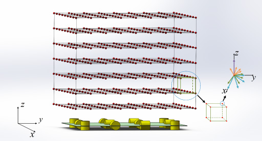The formula for the induced voltage is as follows: $\begin{eqnarray}\displaystyle U^{\ast }(r^{\ast },\hat{\mathbf{r}}^{\ast },\hat{\mathbf{m}},\hat{\mathbf{a}}^{\ast })=\frac{k}{r^{\ast 3}}(3(\hat{\mathbf{m}}\cdot \hat{\mathbf{r}}^{\ast })(\hat{\mathbf{r}}^{\ast }\cdot \hat{\mathbf{a}}^{\ast })-(\hat{\mathbf{m}}\cdot \hat{\mathbf{a}}^{\ast })) & & \displaystyle\end{eqnarray}$ (5) where $\hat{\mathbf{a}}^{\ast }$ is the attitude of the sensing coil in each grid, and r ^∗ is the vector pointing from the center of the transmitting coil to the sensing coil. Additionally, r ^∗ = ∥r ^∗∥, $\hat{\mathbf{r}}^{\ast }=\frac{\mathbf{r}^{\ast }}{r^{\ast }}$ .

Fig. 2.

Local calibration grid selection diagram (the figure selects a vertex of a grid and its 13 different attitudes of the transmitting coil; purple arrow: 𝛽 = 0, orange arrows: 𝛽 = π∕6, green arrows: 𝛽 = π∕3, blue arrows: 𝛽 = π∕2).

For each grid, the problem of solving the parameters of the sensing coil was also transformed into a non-linear least squares problem. $\begin{eqnarray}\displaystyle H_{n,i}(k_{i},U_{i0},{x_{n,i}^{a}}^{\ast },{y_{n,i}^{a}}^{\ast },{z_{n,i}^{a}}^{\ast },{{\varphi}_{n,i}}^{\ast },{{\theta}_{n,i}}^{\ast })=\mathop{\sum }_{j}(U_{n,i}^{\ast j}-U_{n,i}^{\prime j})^{2} & & \displaystyle\end{eqnarray}$ (6) where $({x_{n,i}^{a}}^{\ast },{y_{n,i}^{a}}^{\ast },{z_{n,i}^{a}}^{\ast })$ and (𝜑_{n, i} ^∗, θ_{n, i} ^∗) are the ith sensing coil parameters in the nth grid, $U_{n,i}^{\prime j}$ is the jth induced voltage of ith sensing coil in nth grid, $U_{n,i}^{\ast j}$ is the theoretical value and j is the index of data (j = 8 * number of different attitude of transmitting coil).

2.3. Algorithms

2.3.1. Non-linear least square algorithm

In the process of determining the sensing coil parameters and tracking the transmitting coil, the non-linear least squares algorithm was involved. In this paper, when solving the non-linear least squares problem, the L-M algorithm was adopted [13].

When solving the parameters of the sensing coil, the initial value of the L-M algorithm selects the designed values of sensing coil parameters, which can speed up the convergence of the algorithm and avoid falling into the local minimum. In the process of tracking the transmitting coil, a series of uniformly distributed positions were chosen as initial values of the L-M, and they are arranged according to the law of the distance from the center of the tracking space. During the calculation process, when the calculated residual was higher than the preset value, the initial value was replaced, and this procedure was repeated until the end of calculation.

2.3.2. Iterative GSCPOP calibration method

The iterative GSCPOP calibration algorithm proposed in this paper is to locate the position and orientation of the transmitting coil by iteratively using the position and orientation parameters generated by local calibration, and reduce the influence of magnetic field distortion. The steps of the calibration method are as follows:

(1) The initial values V ₀(x ^m, y ^m, z ^m, 𝛼^m, 𝛽^m) are used as the input (the uniformly selected initial values in the tracking space mentioned in Section 2.3.1);

(2) The L-M algorithm is used to estimate the position and orientation of the transmitting coil for the first time, we obtained V _pre(x ^m, y ^m, z ^m, 𝛼^m, 𝛽^m);

(3) The number of grids in space is judged according to the calculated position in step (2), recorded as N _pre. The calibrated grid parameters are used to track the position and orientation of the transmitting coil again;

Fig. 3.

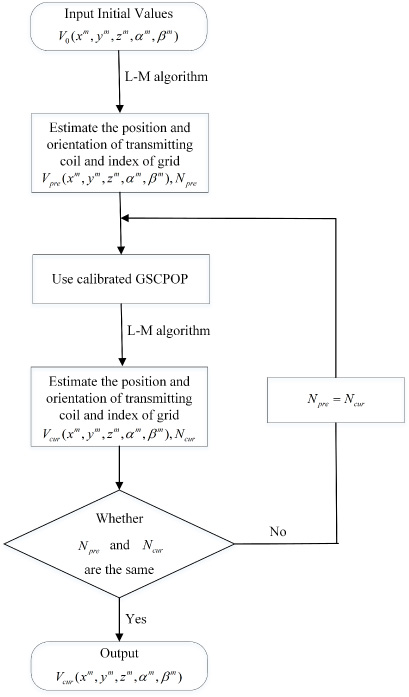
Flowchart of the GSCPOP calibration method.

(4) The grid number is redetermined according to the calculated position in step (3), recorded as N _cur;

(5) If the grid calculated in step (4) and grid in step (3) are the same grid, the calculation stops; otherwise, repeat step (3) and step (4);

(6) If the number of iterations exceeds the threshold, the calculation ends, and returns the information that the tracking result does not converge.

Fig. 4.

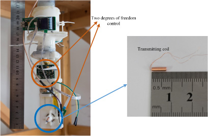
3D printing apparatus and transmitting coil.

Fig. 5.

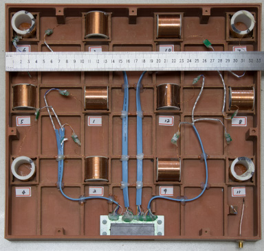
Sensing coil assembly.

Flowchart of the GSCPOP calibration method is appended in Fig. 3.

3. Experiments and results

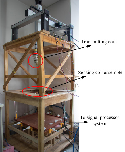
3.1. EMTS experiment setup

The EMTS experimental setup was presented in our previous article [12]. Figure 4 shows the 3D printing apparatus with two degrees of freedom, and a transmitting coil is fixed on it. A Bourns 3547S-1AA-502A angle transducer with a maximum independent linearity error of ±0.25% and a Murata SCA100T-D02 accelerometer with a resolution of 0.0035° are used to measure the orientation of the transmitting coil. Figure 5 shows the sensing coil assembly. Figure 6 shows the signal processor system, and Fig. 7 shows the test platform, with an accuracy of ±0.02 mm and a repeatability of ±0.01 mm.

Fig. 6.

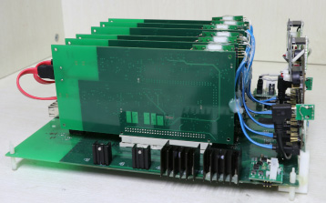
Signal processor system.

Fig. 7.

The test platform.

3.2. Data acquisition

In this study, we collected data twice: once for calculating the position and orientation parameters of the sensing coils, and the other for testing the performance of the calibration method.

Collected data for GSCPOP calibration are as follows.

The motion range of the test platform is 400 mm ∗ 400 mm ∗ 400 mm, and we separate this area every 50 mm. That is, in x and y directions, we collected nine points and in the z direction collected seven points from 0 mm to 300 mm. Therefore, we collected 567 (9 ∗ 9 ∗ 7) points altogether. At each point, we chose 16 orientations of the transmitting coil. These 16 orientations are the combination of two angles because our apparatus has two degrees of freedom, and we chose four angles for each degree. However, when 𝛽 is 0, it is the same to change 𝛼, so there are 13 efficient orientations (Table 1). Therefore, we have 7371 (567 ∗13) different calibration points (Fig. 8).

Table 1
Attitudes of the transmitting coil in the calibration dataset

𝛽 (rad) 𝛼 (rad)

0 0

π∕6 0, π∕6, π∕3, π∕2

π∕3 0, π∕6, π∕3, π∕2

π∕2 0, π∕6, π∕3, π∕2

𝛽 (rad)	𝛼 (rad)
0	0
π∕6	0, π∕6, π∕3, π∕2
π∕3	0, π∕6, π∕3, π∕2
π∕2	0, π∕6, π∕3, π∕2

Fig. 8.

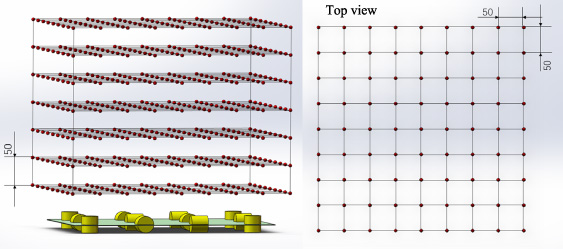
Calibration points diagram and its top view.

Table 2

Attitudes of the transmitting coil in the validation dataset

𝛽 (rad)	𝛼 (rad)
π∕12	π∕4
π∕4	π∕4
5∕12π	π∕2

We also collected data at different points to verify our calibration method. Therefore, we changed the interval of the validation dataset and chose different attitudes of the transmitting coil. In the x and y directions, we collected data every 70 mm from 50 mm to 330 mm, And in z direction, we chose five different heights from 74 mm to 304 mm (74 mm, 124 mm, 184 mm, 244 mm, 304 mm). At each point, we chose three attitudes, as Table 2 shows. Therefore, the total validation data consists of 375 points.

3.3. Evaluation standards

After tracking the transmitting coil, we used Δr to represent the position error between the calculated value and the actual position and Δ𝛼 to represent the orientation error (Fig. 9).

Fig. 9.

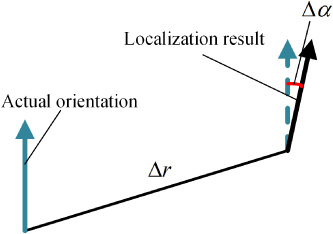
Diagram of position error and orientation error.

To evaluate the improvement in the calibration method on position accuracy and orientation accuracy, we employed the geometric mean 𝛱, the arithmetic mean ϵ, the standard deviation σ, the percentage of data with position error or orientation error less than 3 mm or 3°, respectively, p ₃, and the percentage of data with error less than 10 mm and 10°, respectively, p ₁₀. $\begin{eqnarray}\displaystyle {\Pi}=\exp \left(\frac{1}{m}\mathop{\sum }_{j=1}^{m}\ln {\varepsilon}_{j}\right) & & \displaystyle\end{eqnarray}$ (7) where m is the total number of data.

3.4. Results

We compared the results of three different methods: using theoretical position and orientation values of the sensing coils to locate the transmitting coil (method 1), using the global sensing coil position and orientation parameter calibration method (method 2), and using the iterative GSCPOP calibration method (method 3). A comparison of the position accuracy is shown in Table 3. The single point position accuracy results are shown in Fig. 10. Comparisons of orientation accuracy are shown in Table 4 and Fig. 11.

Table 3
Position accuracy comparison among the three methods

Method 1 Method 2 Method 3

𝛱 (mm) 5.25 3.42 2.18

ϵ (mm) 10.33 6.52 2.68

σ (mm) 23.43 16.68 1.73

p ₃ (%) 26.93% 27.73% 64.53%

p ₁₀ (%) 81.07% 90.93% 1

	Method 1	Method 2	Method 3
𝛱 (mm)	5.25	3.42	2.18
ϵ (mm)	10.33	6.52	2.68
σ (mm)	23.43	16.68	1.73
p ₃ (%)	26.93%	27.73%	64.53%
p ₁₀ (%)	81.07%	90.93%	1

Fig. 10.

Position error distribution among the three methods.

Table 4

Orientation accuracy comparison among the three methods

	Method 1	Method 2	Method 3
𝛱 (°)	3.02	2.40	2.10
ϵ (°)	5.21	3.65	2.28
σ (°)	12.19	8.50	0.88
p ₃ (%)	52.27%	72.80%	85.60%
p ₁₀ (%)	95.47%	97.60%	1

Fig. 11.

Orientation error distribution among the three methods.

Method 3 improved both position accuracy and orientation accuracy compared to the other two methods. Compared with method 1, method 3 showed a 285% improvement in position accuracy and a 129% improvement in orientation accuracy. After several iterations, almost all the results show that method 3 uses the correct GSCPOP to track the transmitting coil.

From the error distribution diagram, method 1 and method 2 show some poor results where the calculated position and orientation of the transmitting coil are far from the real position and orientation due to the non-convergence of the algorithms. Only method 3 does not show very poor results. Poor results from method 1 and method 2 indicate that these two methods cannot completely correct the magnetic field distortion. Method 3 divides the space into many grids in the calibration process and contains the distortion information of the magnetic field in different attitudes of the transmitting coil, which can improve the orientation accuracy of EMTS to a great extent.

4. Discussion

With the help of EMTS to determine the position and shape of endoscopes, this novel tracking system will provide great convenience to doctors during endoscopic insertion surgery, shorten the procedure time, avoid the occurrence of loops, and greatly reduce the suffering of the patient. At the same time, for the patient’s later re-examination, the ability to relocate the lesion is also very helpful.

Fitting the shape of the endoscope usually requires a series of transmitting coils. Only one transmitting coil is discussed in this paper. We can achieve a better reconstruction of the shape of the endoscope by fixing a certain number of transmitting coils into the insertion portion of the endoscope and tracking the positions and orientations of these coils respectively. When we reconstruct only the front end of the endoscope, only one or two transmitting coils are needed, and the orientation information is particularly important.

The usual EMT calibration methods mostly interpolate or use high-order fitting to model the position and orientation errors separately. Our new calibration method, by iterating the GSCPOP, can simultaneously calibrate position and orientation errors. Compared to the uncalibrated method, the iterative GSCPOP calibration method showed a 285% improvement in position accuracy and a 129% improvement in orientation accuracy.

Compared to other calibration methods, such as [14] and [15], our method has obvious advantages. The tracking range of the system in [14] is 250 mm ∗ 200 mm ∗ 100 mm, the position accuracy is 3.3 mm, and the orientation accuracy is 3.0°. The tracking range of the system in [15] is 240 mm ∗ 240 mm ∗ 180 mm, and the position accuracy is 2.15 mm. If we choose the same tracking range, our precision will reach 1.90 mm. Additionally, in comparison to our previous work [12], the complexity of the calibration method is reduced, bringing faster calculation speed, and the correction of orientation error is also added.

Another way to further improve the accuracy of EMTS is to reduce the size of the grid, which can better correct the model error. At the same time, it will extend the calibration procedure. There is a trade-off between tracking accuracy and calibration time.

To adapt to clinical practice, the range of tracking should be larger. We also tested 1000 points from 410 mm to 790 mm along the z axis. The results showed that the iterative GSCPOP calibration method had a 500% improvement in position accuracy and a 76% improvement in orientation accuracy, which can meet the requirements of clinical practice.

However, it should be noted that the calibration method cannot completely remove the influence of metal materials on EMTS, so we need to think of other ways to solve this problem. For example, we could use dual-frequency transmission, or we could combine other sensors (such as three-axis gyroscopes and accelerometers) to correct the error.

5. Conclusion

In this paper, we propose an iterative GSCPOP calibration method. By separately calibrating the sensing coil position and orientation parameters, the position accuracy and orientation accuracy are simultaneously improved. Compared with the uncalibrated method, the proposed calibration method showed a 285% improvement in position accuracy and a 129% improvement in orientation accuracy. In a further tracking range, we also tested our calibration method and achieved good accuracy to meet the requirements of clinical conditions.

Footnotes

Acknowledgements

The authors are grateful to Yishu Hu, Bin Liu, Xiguang Wang, Chenxi Wang, Wentao Yuan and others for valuable discussions.

References

Mancino

M.G.

Bianchi

Festa

Maurizio

and Dezi

, Recent advances in endoscopic management of gastrointestinal cancers, Translational Gastrointestinal Cancer 3 (2014), 80–89, doi:10.3978/j.issn.2224-4778.2013.10.05.

Cleary

and Peters

T.M.

, Image-guided interventions: technology review and clinical applications, Annual Review of Biomedical Engineering 12 (2010), 119–142, doi:10.1146/annurev-bioeng-070909-105249.

Poulin

and Amiot

L.P.

, Interference during the use of an electromagnetic tracking system under OR conditions, Journal of Biomechanics 35 (2002), 733–737, doi:10.1016/S0021-9290(02)00036-2.

Ghazisaedy

Adamczyk

Sandin

D.J.

Kenyon

R.V.

and Defanti

T.A.

, Ultrasonic calibration of a magnetic tracker in a virtual reality space, in: Proc. Virtual Reality International Symposium, 1995, pp. 179–188. doi:10.1109/VRAIS.1995.512494.

Czernuszenko

Daniel

and Defanti

, Line of sight method for tracker calibration in projection-based VR systems, Indian Journal of Chest Diseases & Allied Sciences 28 (1998), 202–211.

Kindratenko

V.V.

and Sherman

W.R.

, Neural network-based calibration of electromagnetic tracking systems, Virtual Reality 9 (2005), 70–78, doi:10.1007/s10055-005-0005-3.

Livingston

M.A.

and State

, Magnetic tracker calibration for improved augmented reality registration, Teleoperators and Virtual Environments 6 (1997), 532–546, doi:10.1162/pres.1997.6.5.532.

Kindratenko

and Bennett

, Evaluation of rotation correction techniques for electromagnetic position tracking systems, in: Proc. Eurographics Workshop, Virtual Environments, Berlin, Germany, pp. 13–22. doi:10.2312/EGVE/EGVE00/013-022.

Kindratenko

, Calibration of electromagnetic tracking devices, Virtual Reality 4 (1999), 139–150, doi:10.1007/BF01408592.

10.

Ikits

Brederson

J.D.

Hansen

C.D.

and Hollerbach

J.M.

, An improved calibration framework for electromagnetic tracking devices, IEEE Computer Society (2001), doi:10.1109/VR.2001.913771.

11.

Zachmann

, Distortion correction of magnetic fields for position tracking, Proc Computer Graphics International (1997), 213–220, doi:10.1109/CGI.1997.601306.

12.

Sun

Xiong

Chen

Han

and Xie

, A locally weighted method for electromagnetic localization of endoscopes, International Journal of Applied Electromagnetics and Mechanics 58 (2018), 387–410, doi:10.3233/JAE-170150.

13.

Meng

M.Q.H.

and Mandal

, Efficient magnetic localization and orientation technique for capsule endoscopy, International Journal of Information Acquisition 2 (2005), 23–36, doi:10.1142/S0219878905000398.

14.

Meng

Q.H.

and Mandal

, The calibration of 3-axis magnetic sensor array system for tracking wireless capsule endoscope, in: Proc. IEEE/RSJ International Conference on Intelligent Robots and Systems, pp. 162–167. doi:10.1109/IROS.2006.282118.

15.

Bien

and Rose

, Algorithm for calibration of the electromagnetic tracking system, in: Proc. IEEE-EMBS International Conference on Biomedical and Health Informatics, pp. 85–88. doi:10.1109/BHI.2012.6211512.

16.

Zachmann

, Virtual reality in assembly simulation – collision detection, simulation algorithms, and interaction techniques, Ph.D. dissertation, University of Bremen, 2000. doi:10.13140/RG.2.2.35200.84482.

A calibration method of position and orientation errors for an endoscopic tracking system

Abstract

Keywords

1. Introduction

2. Principles and methods

2.1. Localization problem

2.2.1. Global calibration of the sensing coil position and orientation parameters

2.3.1. Non-linear least square algorithm

2.3.2. Iterative GSCPOP calibration method

3.1. EMTS experiment setup

Table 1 Attitudes of the transmitting coil in the calibration dataset 𝛽 (rad) 𝛼 (rad) 0 0 π∕6 0, π∕6, π∕3, π∕2 π∕3 0, π∕6, π∕3, π∕2 π∕2 0, π∕6, π∕3, π∕2

Table 3 Position accuracy comparison among the three methods Method 1 Method 2 Method 3 𝛱 (mm) 5.25 3.42 2.18 ϵ (mm) 10.33 6.52 2.68 σ (mm) 23.43 16.68 1.73 p 3 (%) 26.93% 27.73% 64.53% p 10 (%) 81.07% 90.93% 1

5. Conclusion

Footnotes

Acknowledgements

References

Table 1
Attitudes of the transmitting coil in the calibration dataset

𝛽 (rad) 𝛼 (rad)

0 0

π∕6 0, π∕6, π∕3, π∕2

π∕3 0, π∕6, π∕3, π∕2

π∕2 0, π∕6, π∕3, π∕2

Table 3
Position accuracy comparison among the three methods

Method 1 Method 2 Method 3

𝛱 (mm) 5.25 3.42 2.18

ϵ (mm) 10.33 6.52 2.68

σ (mm) 23.43 16.68 1.73

p ₃ (%) 26.93% 27.73% 64.53%

p ₁₀ (%) 81.07% 90.93% 1