Numerical evaluation of focal position selection by line-focusing electromagnetic acoustic transducer with experimental validation

Abstract

As the focal position of a line-focusing electromagnetic acoustic transducer (LF-EMAT) affects the intensity of the focal signal, we measure the displacement signal and the selection method of the focal line position is then studied in this work to improve the signal intensity and detection precision for a shear-vertical (SV) wave LF-EMAT. We calculate the magnetostatics field and bulk wave propagation utilizing the finite element method (FEM). We simulate the characteristics of the SV wave, and we find that the radiant distance and propagation direction has a great influence on the amplitude of the displacement of the specimen. The superposition area of SV waves from different sources possesses better focusing ability, and the triangular area (normalized amplitude of the SV waves lower than 10%) near the surface of a specimen should be avoided to be chosen when designing the meander line coils. As for the line-focusing EMAT described in this manuscript, the selection of focal positions for different thickness specimens or detection depth is completely different. Moreover, we perform an experiment to validate the simulation results and lead to a conclusion that the position of the focal point is required to be appropriately close to the excitation coils to enhance the intensity of the signal, while the best focal position should be calculated.

Keywords

EMAT line focusing focal position selection numerical simulation

1. Introduction

Electromagnetic ultrasonic detection technology is widely used in the industry as a part of ultrasonic guided wave detection technology. As an ultrasonic nondestructive testing (NDT) method, it has great advantages for detecting cracks, interlayers, and folds on the surface or inside the material caused by fatigue, aging, and thermal expansion. The electromagnetic acoustic transducers (EMATs), which use electromagnetic mechanisms for non-contact ultrasound generation and reception, may be expected to replace conventional piezoelectric transducers (PZT) in many applications [1–4]. The contact or couplant between the transducers and the surface of the specimens is not required in an EMAT as the ultrasonic is directly generated within the material adjacent to the transducer. Therefore, it has a wide range of applications for the EMATs such as rough material surface, high temperature and high speed available, etc. [5,6].

Typically, the sensitivity of EMATs is affected by the transmit power, coil turns, constant external magnetic field, electrical conductivity, magnetic permeability and acoustic impedance, which is about 40 dB lower than that of PZTs. The weak transduction efficiency is currently the main challenge of EMATs in practical applications, so different types of signal processing techniques are required to enhance the signal and isolate noise [7–9]. In practical applications, in order to improve the electromagnetic ultrasonic transduction efficiency, a high-power transmitting device with a tuning circuit is required to obtain a strong sound pressure. Moreover, due to the effect of the high transmitting power, there must be a protection device at the input of the receiving circuit. A low noise signal amplifier is also required because the received signal input to the amplifier after two transmissions has a relatively small amplitude (usually at the level of μV). Also, the broad radiation patterns of elastic waves also diminish the ultrasonic energy. It means that the elastic wave generated by an EMAT propagates nearly all the directions in the specimen, which is undesirable for flaw detection purposes. Therefore, many methods of concentrating the wave energy and sharpening the directivity were proposed.

The shear-vertical (SV) wave is generated with longitudinal waves and Rayleigh waves simultaneously by an EMAT and propagates along the oblique direction in the specimen. Contrary to the surface propagation characteristics of the Rayleigh waves [10,11], SV wave EMAT has great advantages in detecting internal and bottom defects of the specimen. Moreover, SV waves focusing is an important method due to the weak transduction efficiency of the transducers. Therefore, in recent years, the proposal and optimization of different focusing methods have attracted more and more attention. Ogi first developed a line-focusing EMAT (LF-EMAT) by changing the spacings of the meander line so that the SV waves generated from all sources become coherent on the focal line [12,13]. The focal line was selected firstly at a fixed frequency, and then the spacings of the meander line are adjusted through an equation. In order to concentrate the SV wave on the focal line, the spacing between the predetermined focal line and the coil segment is an integer multiple of a half wavelength, which is not a constant value at a fixed frequency. The point-focusing EMAT (PF-EMAT) was developed in recent years by utilizing curved meander line coils, then the resolution and intensity of the EMAT were improved [14]. Then the defect detectability of an EMAT has been enhanced by focusing shear waves generated by concentric line sources at a focal point [15]. According to the latest research by Jia in 2018, the effect of the aperture angle of the coils has been investigated as well as the design focal offset for the focusing SV wave EMATs [16]. It should be noted that the selection of the focal line or point is not considered in those works. The driving frequency and the focal position have always been the first step in the implementation of the focusing method, and they are almost ignored in the existing literature. As one of the conditions mentioned above, the selection of the focal position has been investigated in detail herein.

In this manuscript, numerical simulation on the EMAT is achieved by utilizing finite element & multi-physical field methods. The magnetostatics field and bulk wave propagation are investigated by solving the electromagnetic model and the elasto-dynamic model. The effect of different focal lines on the focal intensity is also discussed. Also, normalized amplitudes at different horizontal lines are carefully studied with the change of the focal positions. Simulation and experimental analysis of the SV wave focal position for multi-radiation sources is performed.

2. Model description

Lorenz force is the main force of the ultrasonic excitation for non-ferromagnetic materials. Therefore, in order to study the EMAT, the working process of the transducer is divided into two phases according to the structure of the EMAT. The initial phase is the production process of the Lorenz’s force. The eddy current produced by the electric coil in the specimen generate the Lorenz force under the effect of the external bias magnetic field during this phase. This phase is the conversion process of electromagnetic energy. In the second phase, the specimen effected by the Lorenz force will produce elastic deformation in the interior and surface of the specimen. The vibration and displacement transfer process of the specimen shows the generation and propagation of the ultrasonic wave, and this phase can be described by the elasto-dynamic model.

2.1. Electromagnetic model

The electromagnetic field model corresponds to the first phase of the EMAT. According to the electromagnetics theory, the description of this process utilizes the Maxwell equation and the Lorenz force formula. $\begin{eqnarray}\displaystyle & \displaystyle {\nabla}\times \boldsymbol{H}_{d}=\boldsymbol{J}_{c} & \displaystyle\end{eqnarray}$ (1) $\begin{eqnarray}\displaystyle & \displaystyle \boldsymbol{B}_{d}={\mu}_{m}\boldsymbol{H}_{d} & \displaystyle\end{eqnarray}$ (2) $\begin{eqnarray}\displaystyle & \displaystyle {\nabla}\times \boldsymbol{E}=-\frac{\partial \boldsymbol{B}_{d}}{\partial t} & \displaystyle\end{eqnarray}$ (3) $\begin{eqnarray}\displaystyle & \displaystyle \boldsymbol{J}_{e}={\sigma}\boldsymbol{E} & \displaystyle\end{eqnarray}$ (4) $\begin{eqnarray}\displaystyle & \displaystyle \boldsymbol{F}=\boldsymbol{J}_{e}\times (\boldsymbol{B}_{s}+\boldsymbol{B}_{d}) & \displaystyle\end{eqnarray}$ (5) where H _d is the alternating magnetic field generated by the alternating current in the coils; J _c the conduction current density; B _d the magnetic induction intensity produced by the alternating current; 𝜇_m the relative permeability of the specimen; E the electric field of the eddy current field; J _e the eddy current density; σ the conductivity; B _s the static magnetic field produced by the permanent magnet; F the Lorenz force.

The frequency of the dynamic Lorenz force excited by the dynamic magnetic field generated by the alternating coil is two times that of the static Lorenz force, so the weak dynamic magnetic field can be omitted [17,18].

2.2. Elasto-dynamic model

The ultrasonic wave generated by the EMAT makes the stress and strain of the interior particle of the specimen displaced. The force produced by the displaced particle and the surrounding particle will spread the force, then the ultrasonic wave forms. Therefore, the fundamental equation and wave equation of the elasto-dynamic can describe the second phase of the EMAT. The Lorentz force F in Eq. (5), which is determined by Fleming’s right-hand rule of thumb, is applied as the source term F _v of the elasto-dynamic equation in this model. The Lorentz force calculated by the electromagnetic model affects both the surface and the interior of the specimen in the model. $\begin{eqnarray}\displaystyle & \displaystyle {\rho}\frac{\partial ^{2}\boldsymbol{u}}{\partial t^{2}}={\nabla}\cdot S+\boldsymbol{F}_{v} & \displaystyle\end{eqnarray}$ (6) $\begin{eqnarray}\displaystyle & \displaystyle S=C:{\varepsilon}_{el} & \displaystyle\end{eqnarray}$ (7) $\begin{eqnarray}\displaystyle & \displaystyle C=\left[\begin{array}{@{}cccccc@{}}{\lambda}+2{\mu} & {\lambda} & {\lambda} & 0 & 0 & 0\\ {\lambda} & {\lambda}+2{\mu} & {\lambda} & 0 & 0 & 0\\ {\lambda} & {\lambda} & {\lambda}+2{\mu} & 0 & 0 & 0\\ 0 & 0 & 0 & {\mu} & 0 & 0\\ 0 & 0 & 0 & 0 & {\mu} & 0\\ 0 & 0 & 0 & 0 & 0 & {\mu}\\ \end{array}\right] & \displaystyle\end{eqnarray}$ (8) $\begin{eqnarray}\displaystyle & \displaystyle {\varepsilon}_{el}={\varepsilon}-{\varepsilon}_{inel}=\frac{1}{2}[({\nabla}\boldsymbol{u})^{T}+{\nabla}\boldsymbol{u}]-{\varepsilon}_{inel}. & \displaystyle\end{eqnarray}$ (9)

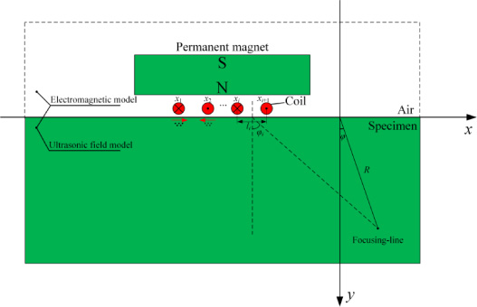
The wave equation shown above equals to the Navier’s equation in the isotropic elastic solid medium though they represent in the different form. Elastic waves displacement of the model is calculated by applying the various properties of the aluminum specimen in this equation. $\begin{eqnarray}\displaystyle ({\lambda}+{\mu}){\nabla}{\nabla}\cdot \boldsymbol{u}+{\mu}{\nabla}^{2}\boldsymbol{u}+\boldsymbol{F}_{v}={\rho}\frac{\partial ^{2}\boldsymbol{u}}{\partial t^{2}} & & \displaystyle\end{eqnarray}$ (10) where u is the displacement vector; t the time; 𝜌 the mass density; S the stress tensor; F _v the volume force vector which can be obtained from the calculation of the Lorenz force in the electromagnetic field model; C the elasticity tensor which relates to the Lame’s constants 𝜆 and 𝜇 of the material; “:” stands for the double-dot tensor product; ϵ_el is the difference between the total strain ϵ and all inelastic strains ϵ_inel, and ϵ_inel = 0 in this manuscript.

Fig. 1.

Two-dimensional schematic diagram of the EMAT in the simulation.

2.3. Model configuration

Schematic diagram of the EMAT is shown in Fig. 1 and a 2-D space is considered here. The permanent magnet is located on the top of the coil and the specimen, the S-pole of the magnet is on the top with the N-pole underneath. The liftoff of the coil in the model is only 25 μm, which can increase the weak coupling efficiency of the EMAT. Coordinates of the coils in the Cartesian coordinate system are (x _i, 0.025 mm) and the distances between the two coils are l _i. In order to facilitate the analysis process, the coordinates of each point in the simulation are corrected. The electromagnetic model is calculated in both air and the specimen while the elasto-dynamic model is utilized in the specimen only.

The fundamental theory of the point-focusing EMAT is developed by Ogi et al. The major radiation angle 𝜑 of the SV waves is determined by the coils’ distances l _i, the wave velocity c and the frequency f of the pulsed current in the coil [19]. $\begin{eqnarray}\displaystyle \sin {\varphi}=\frac{c}{2lf}. & & \displaystyle\end{eqnarray}$ (11)

Then the coordinates of the coils could be calculated using the equation: $\begin{eqnarray}\displaystyle \sin {\varphi}_{i}=\frac{c_{S}}{2l_{i}f}=\frac{|R\sin {\varphi}-x_{i}-l_{i}/2|}{\sqrt{(R\cos {\varphi})^{2}+(R\sin {\varphi}-x_{i}-l_{i}/2)^{2}}} & & \displaystyle\end{eqnarray}$ (12) where the shear wave velocity c _S = (𝜇∕𝜌)^0.5 = 3.2 × 10⁶ mm∕s; f = 1 MHz; 𝜑 = 45°; R = 28.28 mm. Therefore, the coordinates of x ₁, …, x ₁₆ is calculated in this work. Moreover, the focal line locates at (20 mm, 20 mm) in this manuscript.

The excitation current is a burst wave with an amplitude of 3.5 A. The expression of the excitation burst current for the EMAT coils is $\begin{eqnarray}\displaystyle i(t)={\beta}e^{-{\alpha}(t-{\tau})^{2}}\cos [2{\pi}f_{c}(t-{\tau})+{\theta}] & & \displaystyle\end{eqnarray}$ (13) where 𝛽 is the amplitude of the signal, 𝛼 is the bandwidth factor, τ is the arrival time, f _c is the central frequency, and θ is the phase delay. The value of the parameters above is shown in Table 1, and the waveform of the excitation current is shown in Fig. 2.

2.4. Numerical algorithm

The skin effect exists near the surface of the specimen due to the induced current. Therefore, in order to reduce oscillations and overshoots in our simulations, the mesh in the computing area needs to be subdivided carefully. A fine meshing method is utilized in Fig. 3 and the mesh parameters are shown in Table 2. Time steps in this model are automatically determined by the specified relative (0.01) and absolute (0.001) tolerances. Backward Differentiation Formulas are utilized for time differentiation according to the algorithm [20].

Fig. 2.

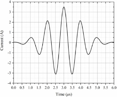
The waveform of the excitation current.

Table 1

Parameters of burst signals for the coils

Parameters	Value
𝛽 (A)	3.5
𝛼	5 × 10¹¹
τ (μs)	3
f _c (MHz)	1
θ (°)	0

Fig. 3.

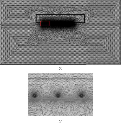
The meshing of the computational domain: (a) Meshing of the overall calculation domain; (b) Meshing of the local calculation domain.

Table 2

Unit dimension parameter of mesh generation

Number of elements	Average element quality	Average growth rates
75478	0.932	1.093

3. Results and discussions

3.1. Magnetostatics field and bulk wave propagation

The static magnetic field produced by permanent magnets is calculated in the steady simulation first, and the distribution of the magnetic field inside the specimen is obtained and shown in Fig. 4. It is shown in this figure that the maximum value of the magnetic flux density exists at the four corners of the permanent magnet. It can be explained that the magnetic lines of force are distributed along the direction of less magnetic reluctance. It can be seen from the changes in the size and direction of the arrow that the magnetic flux density perpendicular to the surface of the specimen is mainly located near the central position of the permanent magnet. Therefore, the tangent Lorenz force that forms the SV wave mainly exists in this area.

Fig. 4.

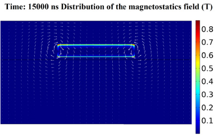
Distribution of the magnetostatics field.

The induced current of the pulse current in the coil is calculated in the specimen and the Lorenz force at each point inside the specimen can be obtained when taken the calculated magnetostatics field above as the background magnetic field. Then the Lorenz force is applied to the aluminum material and the stress, strain and displacement of the specimen are calculated. The transient calculation method is utilized at this stage and the total time of the simulation is 15 μs.

In order to indicate the amplitude and the direction of the displacements of each point in the specimen clearly, the simulation result at 5 μs, 10 μs, and 15 μs is taken as a special case and shown in Fig. 5(a–i).

As shown in Fig. 5(a–c), the displacement in the specimen decreases when far away from the surface, and the maximum value of the displacement exists around the middle of the specimen’s surface. Due to the influence of the periodic Lorenz force, the SV wave will propagate in two directions. Therefore, it can be proved in this figure that the propagation direction of the SV waves is approximately symmetric of the center line and spread obliquely. Figure 5(d–f) shows the distribution of the displacement field when the coil has constant spaces of 2.3 mm. It can be seen from the figure that there is mutual interference and superposition between the various radiation sources. Compared with the figure, the focusing coil is utilized in Fig. 5(g–i). It can be clearly seen that the amplitude of the displacement at the focal point is large, which proves the existence of the focusing effects.

For comparison purposes, uniformly-spaced coils are utilized in another simulation, which has a constant space of 2.3 mm shown in Fig. 5(d–f). When other conditions remain unchanged, the displacements at the same point (focal line) are shown in Fig. 6. It can be seen from the figure that the LF-EMAT successfully focused the SV wave at the position as expected while the uniformly-spaced EMAT has a smaller displacement amplitude than the LF-EMAT.

Fig. 5.

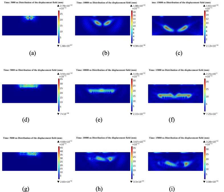
Distribution of the displacement field at 5000 ns, 10000 ns, and 15000 ns: (a–c) Single-source EMAT, (d–f) Constant-spaced EMAT and (g–i) Focusing EMAT.

The direction of the transverse wave is perpendicular to the direction of the vibration, then the amplitude of the SV wave cannot be obtained accurately by the calculation of total displacement above.

Fig. 6.

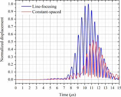
The displacements at the same point (focal line) radiated by LF-EMAT and constant-spaced EMAT.

Fig. 7.

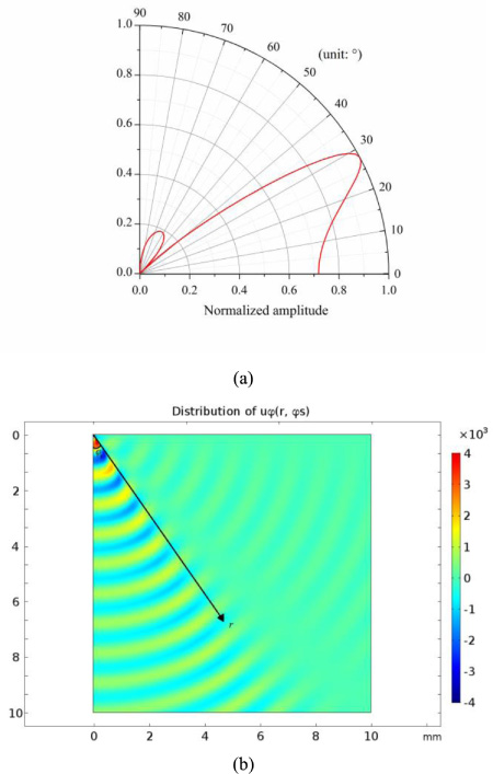
The normalized amplitude and phase distribution of u _𝜑 generated from a line source; (a) Normalized amplitude at different propagation angles of SV waves and (b) Distribution of u _𝜑(r, 𝜑_S) in a 2-D plane.

3.2. Selection of focal position

The displacement u _𝜑 of the SV wave generated by a strip source is perpendicular to the propagation direction and can be expressed as follows [21]. $\begin{eqnarray}\displaystyle & \displaystyle u_{{\varphi}}(r,{\varphi}_{S})=\frac{C}{\sqrt{r}}\frac{({\lambda}+2{\mu})\cos 2{\varphi}_{S}\cos {\varphi}_{S}}{2{\mu}\sin 2{\varphi}_{S}\sin {\varphi}_{L}\cos {\varphi}_{L}+({\lambda}+2{\mu})\cos ^{2}2{\varphi}_{S}}e^{j[(3/4){\pi}-k_{S}r]} & \displaystyle\end{eqnarray}$ (14) $\begin{eqnarray}\displaystyle & \displaystyle \cos ^{2}{\varphi}_{L}=1-\left(\frac{{\lambda}+2{\mu}}{{\mu}}\right)\sin ^{2}{\varphi}_{S} & \displaystyle\end{eqnarray}$ (15) where C is a constant; 𝜆 and 𝜇 are Lame’s constants which equals to 58 GPa and 26 GPa respectively; k _S = ω∕c _S is wave number of the SV wave; 𝜑_s is the SV wave’s propagation direction; 𝜑_L is the angle of the longitudinal wave. The normalized amplitude and phase distribution of u _𝜑 generated from a line source is shown in Fig. 7(a,b). It is obtained from Fig. 7(a) that there is a maximum value at around 28° and beyond which the amplitude drops. According to Fig. 7(b), we can conclude that the radiant distance has a great influence on the amplitude of the displacement u _𝜑. In previous studies, the focal line is selected firstly as a prerequisite. However, the effect of different focal positions does not fully consider by these papers. Therefore, it is necessary to select a better radiant angle and distance of the SV waves to improve the efficiency of the EMAT.

According to the equation $\begin{eqnarray}\displaystyle \sin {\varphi}=\frac{c}{2lf}=\frac{3.2∼\text{km}/\text{s}}{2\times 10^{6}/s\times l}=\frac{1.6}{l}. & & \displaystyle\end{eqnarray}$ (16)

Therefore, in order to generate the SV wave, the spaces of the coils l _i > 1.6 mm should be satisfied. In this manuscript, the radiant point refers to the center point at which the eddy currents induced by two adjacent coils on the surface of the specimen. The distance a between the two radiant points of SV waves satisfies equation a > (l _i + l _i+1)∕2 > 1.6 mm. To simplify the process of the simulation, two radiate points are utilized to calculate the equation u _𝜑(r, 𝜑_S). One point locates at the origin of the coordinates, and another point locates at a distance of a from the first one. Here a is chosen as 2 mm, 3 mm and 4 mm as three cases, and the calculation data is normalized to facilitate the comparison. The distribution of the normalized amplitude represents the focusing efficiency. Although the maximum SV wave intensity appears near the surface of the specimen, it is hard to put into use in the practice. Therefore, the reasonable efficiency values 10%–30% are chosen and shown as contour lines in Fig. 8(a–c). Assume that the efficiency value of 20% is acceptable in this manuscript, the distributions of different a are shown in Fig. 8(d–f).

Fig. 8.

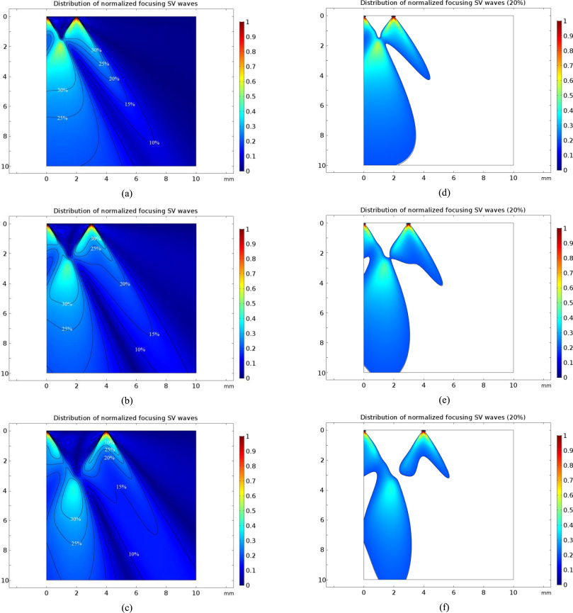
Distribution of normalized focusing SV waves; (a) a = 2 mm, (b) a = 3 mm, (c) a = 4 mm, (d) a = 2 mm (20%), (e) a = 3 mm (20%) and (f) a = 4 mm (20%).

We can conclude from Fig. 8(a–f) that the selection of the focal line’s position is significant to improve the efficiency of the EMATs. It is known that the SV waves propagate symmetrically in two directions, so the superposition area of SV waves from different sources possesses the better focusing ability. As the distance a increases, the overall focusing level in the region has been reduced, and the “effective area” is also narrowed. It should be noticed that in a triangular area near the surface of a specimen, the amplitude of the SV wave is shown extremely weak. Therefore, the focal line should be avoided to set here.

Fig. 9.

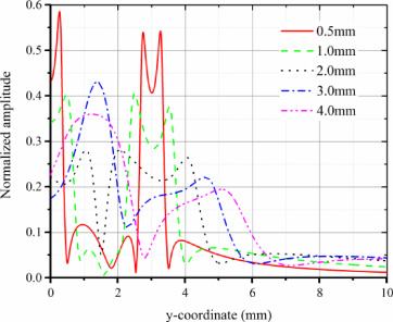
Normalized amplitudes at different horizontal lines.

The LF-EMAT was usually utilized in the detection of shallow notch on the surface of an aluminum block, and the focal line always located on the surface of the block. In order to investigate the influence of the focal position, 5 horizontal lines at different positions (y = 0.5 mm, 1.0 mm, 2.0 mm, 3.0 mm, 4.0 mm) are selected when the distance fixed at a = 3 mm. Normalized amplitudes along each horizontal line are shown in Fig. 9. We can conclude from this figure that the amplitude along each horizontal line shows common characteristics. The two peaks in the figure are both below the radiate points and the amplitude decreases when the focal line moves far away. As the intensity of the SV wave is related to the direction of radiation and it is proved that there is a maximum value at around 28°. Therefore, there are two symmetrical peaks at the maximum amplitude under each radiation source. Moreover, Due to the superposition of the waves, the maximum value appears in the middle of the two radiant points when y = 3 mm. We can conclude that the position of the focal line should be chosen near the radiation point when the aluminum block is thin enough. However, the focal line needs to be located at the middle of the radiation points when the thickness of the aluminum plate is larger than 4 mm.

3.3. Experiment

A simple model of two radiation sources is studied above, and the influence of the focal position selection on the intensity of the focused signal is analyzed when the specimen is thin. However, the number of the meander line coils should be more to ensure that the signal is strong enough in the practical application of defect detection, and the thickness of the aluminum block is larger. Moreover, changes in the focal position also lead to the change of the coil spacing, which is more complicated for the analysis. Therefore, simulation and experimental analysis of the SV wave focus position for multi-radiation sources are also important. The schematic diagram of the experimental setup is shown in Fig. 10.

Fig. 10.

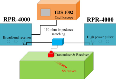
Experimental configuration for the SV wave EMAT.

The signal generation and reception in the experiment are modulated and amplified before being processed for signal generation purposes. Therefore, RPR-4000 pulser/receiver is selected in the experiment. The coils inside the transmitter and the receiver are well-designed and made by the PCB method. The arrangement of the coils in the experiment is a meanderline coil structure. The material of the specimen is aluminum, and the size is 150 × 50 × 50 mm³ in the experiment, and the coils are excited by a burst current with an amplitude of 3.5 A and bandwidth factor of 5 ×10¹¹, which can be controlled by the RPR-4000 power and the programming method. The focal point and structures of the transmitter and the receiver are the same, and the experimental conditions are consistent with the simulation conditions. Due to the low energy conversion efficiency of EMAT, high-power pulse current excitation is required. Therefore, in order to obtain the maximum output power of the excitation source, it is required to match the impedance of the load with the internal impedance of the excitation source, then 150 ohms matching impedance are utilized in the experiment to improve the accuracy and the efficiency of the EMAT.

Fig. 11.

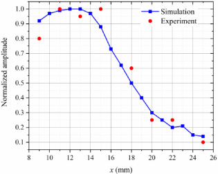
Normalized amplitude of the displacement signal at different x-coordinates of the focal point position.

In the defect detection, the position of the defect is generally on the surface of the specimen. Therefore, the y coordinate of the focal point should be kept constant when selecting the focal position, and the absolute value of the y coordinate is equal to the thickness of the specimen. The effect of the focal position can also be explained as the effect of the horizontal distance between the first coil and the focal point position on the signal intensity. Therefore, it is only necessary to study the relationship between the x coordinate at the focal point and the intensity of the focused signal when the position of the first coil x ₁ (−20 mm, 0.025 mm) is determined. Since the number of coils also affects the intensity of the signal, the number of the coils is fixed to 10 in both simulation and experiment. In this study, different focal positions with different coil spacings are investigated. The relationship between the normalized amplitudes of the SV waves and the x coordinates of the focal points in both simulation and experiment is shown in Fig. 11. It can be seen that the intensity of the signal decreases as the x coordinate increases non-linearly when x > 12 mm, and the phenomenon is different when x < 12 mm. Moreover, the experiment results show good agreement with the simulation results. The amplitude of the signal reaches a peak at x = 12 mm, and it is found by calculation that the radiation angle of the radiation source, which is closest to the focal point, is about 30° in this study. Therefore, it can be concluded that when designing the coil structure of the transducer, the position of the focal point is required to be appropriately close to the excitation coils, and the best focal point is then selected after the calculation.

4. Summary and conclusions

In summary, in order to study the effect of the focal position selection, an electromagnetic model coupled with an elasto-dynamic model are simulated to analyze the characteristics of the line-focusing EMAT. The magnetostatics field and bulk wave propagation are calculated and analyzed utilizing the finite element method. The displacement distribution of the specimen is shown under the burst driven current, which proves the symmetric propagation direction of the SV waves. We conclude from the simulation result that the selection of the focal line’s position is significant to improve the efficiency of the EMATs. For thin aluminum blocks, as the distance between the two radiate points increases, the overall focusing level in the region has been reduced, and the “effective area (20% normalized amplitude)” is also narrowed. It is proved that the focal line should not be located in a triangular area around the surface of the specimen. Moreover, the position of the focal line should be chosen near the radiation point when the aluminum block is thin, while it should be located at the middle of the radiation points when the aluminum block is thicker. Although 30° radiation angle will result in higher signal intensity for a thick plate in the experiment, different focal points can affect the distribution of all the radiant points (or coils), so we perform the simulation and experiment. The simulation agrees well with the experiment and the overall error is less than 10%. We lead to a conclusion that the position of the focal point is required to be appropriately close to the excitation coils to enhance the intensity of the signal, while the best focal position should be calculated. Therefore, it is significant to process the necessary calculation before selecting the focal line.

Footnotes

Acknowledgements

This research was supported by the National Key R&D Program of China (Grant No. 2018YFC0809002), National Natural Science Foundation of China (NSFC) (No. 51677093) and National Natural Science Foundation of China (NSFC) (No. 51777100).

References

Wang

Huang

Wang

and Zhao

, Characterizing excitability of Lamb waves generated by electromagnetic acoustic transducers with coupled frequency domain models, Ultrasonics 93 (2019), 71–80.

Jafarishapoorabadi

Konrad

and Sinclair

, The governing electrodynamic equations of electromagnetic acoustic transducers, J. Appl. Phys. 97 (2005), 2081.

Zhang

Huang

S.L.

Wang

Wei

, Recognition of overlapped lamb wave detecting signals in aluminum plate by EMD-based STFT flight time extraction method, International Journal of Applied Electromagnetics and Mechanics 52 (2016), 991–998.

Zhang

Huang

S.L.

Zhao

Shen

and Wang

, Electromagnetic ultrasonic guided wave long-term monitoring and data difference adaptive extraction method for buried oil-gas pipelines, International Journal of Applied Electromagnetics and Mechanics 54 (2017), 329–339.

Wei

Huang

S.L.

Wang

, Magnetostriction-based omni-directional guided wave transducer for high-accuracy tomography of steel plate defects, IEEE Sens. J. 15 (2015), 6549–6558.

Wang

Huang

S.L.

Zhang

, Multiphysics modeling of a Lorentz force-based meander coil electromagnetic acoustic transducer via steady-state and transient analyses, IEEE Sens. J. 16 (2016), 6641–6651.

Wang

Chen

, Numerical and experimental analysis of unidirectional meander-line coil electromagnetic acoustic transducers, IEEE Trans. Ultrason. Ferr. 60 (2013), 2657–2664.

Dhayalan

and Balasubramaniam

, A two-stage finite element model of a meander coil electromagnetic acoustic transducer transmitter, Nondestr. Test. Eval. 26 (2011), 101–118.

Jian

Dixon

Grattan

K.T.V.

, A model for pulsed Rayleigh wave and optimal EMAT design, Sens. Actuators, A 128 (2006), 296–304.

10.

Thring

C.B.

Fan

and Edwards

R.S.

, Multi-coil focused EMAT for characterization of surface-breaking defects of arbitrary orientation, NDT E Int 88 (2017), 1–7.

11.

Thring

C.B.

Fan

and Edwards

R.S.

, Focused Rayleigh wave EMAT for characterisation of surface-breaking defects, NDT E Int 81 (2016), 20–27.

12.

Ogi

Hirao

and Ohtani

, Line-focusing of ultrasonic SV wave by electromagnetic acoustic transducer, J. Acoust. Soc. Am. 103 (1998), 2411–2415.

13.

Ogi

Hirao

and Ohtani

, Line-focusing electromagnetic acoustic transducers for the detection of slit defects, IEEE Trans. Ultrason. Eng. 46 (1999), 341.

14.

Nakamura

Ashida

Takishita

, Inspection of stress corrosion cracking in welded stainless steel pipe using point-focusing electromagnetic-acoustic transducer, NDT E Int 83 (2016), 88–93.

15.

Takishita

Ashida

Nakamura

, Development of shear-vertical-wave point-focusing electromagnetic acoustic transducer, Jpn. J. Appl. Phys. 54 (2015), 07HC04.

16.

Jia

X.J.

and Qi

Q.Y.

, Influence of aperture angles and design focal depths on the performance of point-focusing shear vertical wave electromagnetic acoustic transducers, J. Acoust. Soc. Am. 143 (2018), 2892–2900.

17.

Mirkhani

Chaggares

Masterson

, Optimal design of EMAT transmitters, NDT E Int 37 (2004), 181–193.

18.

Hao

Huang

Zhao

, Analytical modelling and calculation of pulsed magnetic field and input impedance for EMATs with planar spiral coils, NDT E Int 44 (2011), 274–280.

19.

Moran

T.J.

and Panos

R.M.

, Electromagnetic generation of electronically steered ultrasonic bulk waves, J. Appl. Phys. 47 (1976), 2225–2227.

20.

Gear

, Numerical Initial Value Problems in Ordinary Differential Equations, Prentice Hall, Englewood Cliffs, NJ, 1971.

21.

Miller

G.F.

and Pursey

, The field radiation impedance of mechanical radiators on the free surface of a semi-infinite isotropic solid, Proc. R. Soc. London, Ser. A 223 (1954), 521–541.