Movable and immovable magnets for two machines

Abstract

In this article, the mathematical model of a machine with eight immovable magnets and two movable magnets, and the machine with four immovable magnets and two movable magnets are introduced for the electricity creation. The proposed machines are based on the machine with two immovable magnets and two movable magnets, but they have two main differences: they have more interactions between the immovable and movable magnets, and they create more electricity. Experiments are included to validate that the proposed mathematical models represent a prototype and to observe which machine creates more electricity.

Keywords

Machines immovable magnets movable magnets electricity creation mathematical models

1. Introduction

In these days, the term free-energy is utilized in processes which can obtain energy from the environment, avoiding the necessity of a kind of fuel. Now, some of the most important free-energy processes can be classified in: machines, wind turbines, or solar generators. This article is focused on the machines. The machines of this article utilize the interactions between their immovable and movable magnets for the electricity creation.

There are interesting investigations in magnets processes. In [1–5], the magnet properties of materials are addressed. Magnet sensors are mentioned in [6–10]. In [11,12], magnet navigation is established. Magnet motors are developed in [13,14]. In [15–20], magnet machines are studied. The aforementioned research shows that the magnets processes are a novel topic.

The drawback in the machines is that they need the electricity as a fuel, or in the other case, the machines create electricity during some time until they stop. In this article, two mathematical models of machines are introduced in which the number of immovable magnets is increased with the purpose to increase the electricity creation. The proposed mathematical model is detailed by differential equations and it is based on the parallel axis theorem to obtain the inertia model, the Euler–Lagrange strategy to obtain the mechanic model, and the Kirchhoff voltage law to obtain the electric model. Experiments are included to validate that the proposed mathematical models represent the prototype and to observe which machine creates more electricity. This prototype is transformed to represent each of the proposed machines.

The other sections are described in the next sentence. Section 2 describes the Euler–Lagrange strategy to obtain the mathematical models of machines. Section 3, introduces the mathematical model of the machine with four immovable magnets and two movable magnets. Section 4, proposes the mathematical model of the machine with eight immovable magnets and two movable magnets. Section 5 shows the comparisons between the two machines. The conclusion and future work are explained in Section 6.

2. The Euler–Lagrange strategy to obtain the mathematical models of machines

The equation to be solved by the Euler–Lagrange strategy to obtain the mathematical models of machines is: $\begin{eqnarray}\displaystyle \begin{array}{@{}l@{}}{\tau}={\displaystyle \frac{d}{dt}}\left({\displaystyle \frac{\partial N_{1}}{\partial \dot{{\alpha}}}}\right)-\left({\displaystyle \frac{\partial N_{1}}{\partial {\alpha}}}\right)+{\displaystyle \frac{d}{dt}}\left({\displaystyle \frac{\partial N_{2}}{\partial \dot{{\alpha}}}}\right)-\left({\displaystyle \frac{\partial N_{2}}{\partial {\alpha}}}\right)+b\dot{{\alpha}}\\[10.0pt] N_{1}=J_{1}-W_{1},\quad N_{2}=J_{2}-W_{2}\end{array} & & \displaystyle\end{eqnarray}$ (1) where τ is the torque produced by the interaction of magnets, N ₁ is the is the Lagrangian produced by a movable magnet 1, N ₂ is the Lagrangian produced by a movable magnet 2, J ₁ is the kinetic energy produced by a movable magnet 1, J ₂ is the kinetic energy produced a the movable magnet 2, W ₁ is the potential energy produced by a movable magnet 1, W ₂ is the potential energy produced by a movable magnet 2, b is the damping coefficient of movable magnets.

The procedure to obtain all the mathematical models of machines is:

Energies J ₁, J ₂, W ₁, W ₂ will be gotten as: a) the interactions of all immovable magnets and the movable magnet 1 are used to obtain J ₁, W ₁, b) the interaction between all immovable magnets and the movable magnet 2 are used to obtain J ₂, W ₂.

Energies J ₁, W ₁ will be substituted in the second part of Eq. (1) to obtain N ₁.

Energies J ₂, W ₂ will be substituted in the third part of Eq. (1) to obtain N ₂.

Lagrangians N ₁, N ₂ will be substituted in first part of Eq. (1) to obtain τ.

3. Mathematical model of the machine with four immovable magnets and two movable magnets

The mathematical model of the machine of this section is based on the interaction of two movable magnets with four immovable magnets to obtain a mechanic motion, and the mechanic motion is converted to electricity via an electric generator. Figure 1 shows the full machine with four immovable magnets and two movable magnets. The operation of this mechanism is explained in the next sentence. Immovable is for all parts which do not present motion, and Movable is for all parts which present motion. The immovable platform is to hold the movable and immovable magnets, movable links, and movable arrow, while the immovable structure is to hold the immovable stator and movable arrow. Movable magnets have motion because they interact with immovable magnets. Movable link 1 and movable link 2 have rotations around their joint because in one side they are joined each other, and in the other side they are joined to the two movable magnets. The movable arrow is joined to the joint of movable link 1 and movable link 2; consequently, the rotation of the movable link 1 and movable link 2 yield the rotation of the movable arrow. The movable arrow is the first part of the electric generator, the second part of the electric generator is the immovable stator. The rotation of the movable arrow yields electricity inside of the immovable stator. Then, the operation of the explained mechanism starts with the magnetism produced by interaction between the two movable and four immovable magnets and it finishes with the electricity produced by the immovable stator.

Fig. 1.

Machine with four immovable magnets and two movable magnets.

3.1. The mechanic model

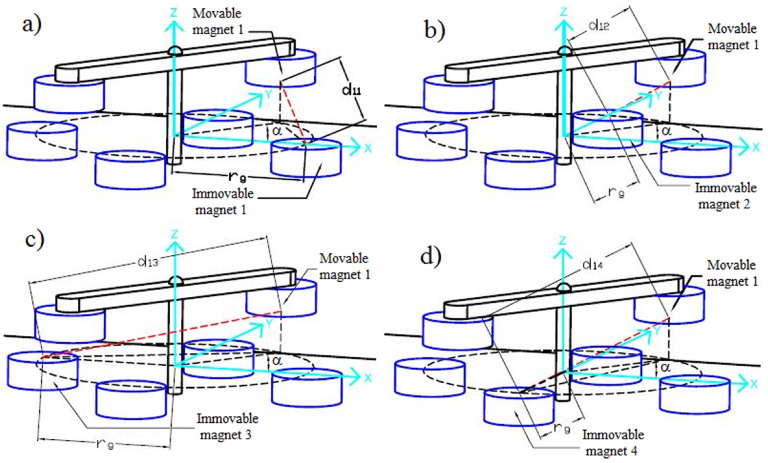
Figure 2 shows four views for the interaction of the movable magnet 1 with respect to the immovable magnet 1 in a), the immovable magnet 2 in b), the immovable magnet 3 in c), and the immovable magnet 4 in d), where some of the main variables are described.

Fig. 2.

Interaction between the movable magnet 1 and the four immovable magnets.

Figure 1 and Fig. 2 show the machine. By using the inertia, the kinetic energy of the movable magnet 1 J ₁ is: $\begin{eqnarray}\displaystyle J_{1}=\frac{1}{2}I_{1}\dot{{\alpha}}^{2}, & & \displaystyle\end{eqnarray}$ (2) where I ₁ is the inertia produced by the movable magnet 1 and $\dot{{\alpha}}$ is the angular velocity of the movable magnet 1. Utilizing the section which take the movable magnet 1, the inertia produced by the link 1 I _e1 is represented as: $\begin{eqnarray}\displaystyle I_{e1}=\frac{1}{12}m_{e1}\left(a_{1}^{2}+c_{1}^{2}\right) & & \displaystyle\end{eqnarray}$ (3) where m _e1 is the mass of the link 1, a ₁ is the width of the link 1, and c ₁ is the length of the link 1. The inertia of the movable magnet 1 I _i1 is: $\begin{eqnarray}\displaystyle I_{i1}=\frac{1}{2}m_{i}r_{i}^{2} & & \displaystyle\end{eqnarray}$ (4) where m _i is the mass of the movable magnet 1, and r _i is the radius of movable magnet 1. Utilizing the parallel axis theorem, the inertia is: $\begin{eqnarray}\displaystyle I=\overline{I}+mr_{g}^{2} & & \displaystyle\end{eqnarray}$ (5) where I is the inertia of Eqs (3) or (4), m is the mass of Eqs (3) or (4), and r _g is the radius of the body rotation. Applying (5) to (3) and (4) gives: $\begin{eqnarray}\displaystyle I_{eu}=\frac{1}{12}m_{e1}(a_{1}^{2}+c_{1}^{2})+m_{e1}r_{g}^{2},\quad I_{iu}=\frac{1}{2}m_{i}r_{i}^{2}+m_{i}r_{g}^{2} & & \displaystyle\end{eqnarray}$ (6) where I _eu is the inertia produced in the link 1, I _iu is the inertia produced in the movable magnet 1, The inertia produced for the movable magnet 1 I ₁ is: $\begin{eqnarray}\displaystyle I_{1}=I_{eu}+I_{iu},\quad I_{1}=\frac{1}{12}m_{e1}(a_{1}^{2}+c_{1}^{2})+m_{e1}r_{g}^{2}+\frac{1}{2}m_{i}r_{i}^{2}+m_{i}r_{g}^{2}. & & \displaystyle\end{eqnarray}$ (7) Substituting the inertia produced for the movable magnet 1 in the kinetic energy of the movable magnet 1 J ₁, gives: $\begin{eqnarray}\displaystyle J_{1}=\left(\frac{1}{24}m_{e1}(a_{1}^{2}+c_{1}^{2})+\frac{1}{2}m_{e1}r_{g}^{2}\right)\dot{{\alpha}}^{2}+\left(\frac{1}{4}m_{i}r_{i}^{2}+\frac{1}{2}m_{i}r_{g}^{2}\right)\dot{{\alpha}}^{2}. & & \displaystyle\end{eqnarray}$ (8) Taking a similar procedure, J ₂ is: $\begin{eqnarray}\displaystyle J_{2}=\left(\frac{1}{24}m_{e2}(a_{2}^{2}+c_{2}^{2})+\frac{1}{2}m_{e2}r_{g}^{2}\right)\dot{{\alpha}}^{2}+\left(\frac{1}{4}m_{i}r_{i}^{2}+\frac{1}{2}m_{i}r_{g}^{2}\right)\dot{{\alpha}}^{2}. & & \displaystyle\end{eqnarray}$ (9) For the Lagrangian N ₁, the potential energy W ₁ for the movable magnet 1 is gotten by the Fig. 1 and Fig. 2: $\begin{eqnarray}\displaystyle W_{1}=\frac{B_{11}^{2}}{2{\mu}}V_{11}+\frac{B_{12}^{2}}{2{\mu}}V_{12}+\frac{B_{13}^{2}}{2{\mu}}V_{13}+\frac{B_{14}^{2}}{2{\mu}}V_{14}=\frac{B^{2}}{2{\mu}}V_{11}+\frac{B^{2}}{2{\mu}}V_{12}+\frac{B^{2}}{2{\mu}}V_{13}+\frac{B^{2}}{2{\mu}}V_{14}, & & \displaystyle\end{eqnarray}$ (10) B ₁₁ = B _m1 + B _f1 is the magnet flux density presented in the volume created by the movable magnet 1 and immovable magnet 1, B ₁₂ = B _m1 + B _f2 is the magnet flux density presented in the volume of the movable magnet 1 and immovable magnet 2, B ₁₃ = B _m1 + B _f3 is the magnet flux density presented in the volume of the movable magnet 1 and immovable magnet 3, B ₁₄ = B _m1 + B _f4 is the magnet flux density presented in the volume of the movable magnet 1 and immovable magnet 4, since all magnets are equal B ₁₁ = B ₁₂ = B ₁₃ = B ₁₄ = B,V ₁₁ is the volume of the movable magnet 1 and immovable magnet 1, V ₁₂ is the volume of the movable magnet 1 and immovable magnet 2, V ₁₃ is the volume of the movable magnet 1 and immovable magnet 3, V ₁₄ is the volume of the movable magnet 1 and immovable magnet 4, μ is the magnet permeability constant in magnets. From Fig. 1 and Fig. 2, volumes and distances are: $\begin{eqnarray}\displaystyle \begin{array}{@{}l@{}}V_{11}={\pi}r_{i}^{2}d_{11},\quad V_{12}={\pi}r_{i}^{2}d_{12},\quad V_{13}={\pi}r_{i}^{2}d_{13},\quad V_{14}={\pi}r_{i}^{2}d_{14},\\[6.0pt] d_{11}=(x_{11}^{2}+y_{11}^{2}+z_{11}^{2})^{0.5},\quad d_{12}=(x_{12}^{2}+y_{12}^{2}+z_{12}^{2})^{0.5},\\[6.0pt] d_{13}=(x_{13}^{2}+y_{13}^{2}+z_{13}^{2})^{0.5},\quad d_{14}=(x_{14}^{2}+y_{14}^{2}+z_{14}^{2})^{0.5},\end{array} & & \displaystyle\end{eqnarray}$ (11) r _i is the radius of the surface in the magnet, d ₁₁ is the centers distance of the movable magnet 1 and immovable magnet 1, d ₁₂ is the centers distance of the movable magnet 1 and immovable magnet 2, d ₁₃ is the centers distance of the movable magnet 1 and immovable magnet 3, d ₁₄ is the centers distance of the movable magnet 1 and immovable magnet 4, x ₁₁, y ₁₁, z ₁₁ are parts of the distance d ₁₁, x ₁₂, y ₁₂, z ₁₂ are parts of the distance d ₁₂, x ₁₃, y ₁₃, z ₁₃ are parts of the distance d ₁₃, and x ₁₄, y ₁₄, z ₁₄ are parts of the distance d ₁₄, where: $\begin{eqnarray}\displaystyle \begin{array}{@{}l@{}}x_{11}=r_{g}(1-\cos {\alpha}),\quad x_{12}=x_{14}=r_{g}\cos {\alpha},\quad x_{13}=r_{g}(1+\cos {\alpha}),\\[4.0pt] y_{11}=y_{13}=r_{g}\sin {\alpha},\quad y_{12}=r_{g}(1-\sin {\alpha}),\quad y_{14}=r_{g}(1+\sin {\alpha}),\\[4.0pt] z_{11}=z_{12}=z_{13}=z_{14}=h,\end{array} & & \displaystyle\end{eqnarray}$ (12) r _g is the radius of movable magnets, h is the distance of a movable magnet and a immovable magnet on the axis z. Substituting (12) in (11) is: $\begin{eqnarray}\displaystyle \begin{array}{@{}l@{}}d_{11}=[r_{g}^{2}(1-\cos {\alpha})^{2}+r_{g}^{2}(\sin {\alpha})^{2}+h^{2}]^{0.5}=[2r_{g}^{2}(1-\cos {\alpha})+h^{2}]^{0.5},\\[6.0pt] d_{12}=[r_{g}^{2}(\cos {\alpha})^{2}+r_{g}^{2}(1-\sin {\alpha})^{2}+h^{2}]^{0.5}=[2r_{g}^{2}(1-\sin {\alpha})+h^{2}]^{0.5},\\[6.0pt] d_{13}=[r_{g}^{2}(1+\cos {\alpha})^{2}+r_{g}^{2}(\sin {\alpha})^{2}+h^{2}]^{0.5}=[2r_{g}^{2}(1+\cos {\alpha})+h^{2}]^{0.5},\\[6.0pt] d_{14}=[r_{g}^{2}(\cos {\alpha})^{2}+r_{g}^{2}(1+\sin {\alpha})^{2}+h^{2}]^{0.5}=[2r_{g}^{2}(1+\sin {\alpha})+h^{2}]^{0.5}.\\[6.0pt] V_{11}={\pi}r_{i}^{2}[2r_{g}^{2}(1-\cos {\alpha})+h^{2}]^{0.5},\quad V_{12}={\pi}r_{i}^{2}[2r_{g}^{2}(1-\sin {\alpha})+h^{2}]^{0.5},\\[6.0pt] V_{13}={\pi}r_{i}^{2}[2r_{g}^{2}(1+\cos {\alpha})+h^{2}]^{0.5},\quad V_{14}={\pi}r_{i}^{2}[2r_{g}^{2}(1+\sin {\alpha})+h^{2}]^{0.5}.\end{array} & & \displaystyle\end{eqnarray}$ (13) Substituting the equation (13) in the potential energy W ₁ of the equation (10) is: $\begin{eqnarray}\displaystyle W_{1} & = & \displaystyle \frac{B^{2}}{2{\mu}}{\pi}r_{i}^{2}[2r_{g}^{2}(1-\cos {\alpha})+h^{2}]^{0.5}+\frac{B^{2}}{2{\mu}}{\pi}r_{i}^{2}[2r_{g}^{2}(1-\sin {\alpha})+h^{2}]^{0.5}\nonumber\\ \displaystyle \text{} & \text{} & \displaystyle +∼\frac{B^{2}}{2{\mu}}{\pi}r_{i}^{2}[2r_{g}^{2}(1+\cos {\alpha})+h^{2}]^{0.5}+\frac{B^{2}}{2{\mu}}{\pi}r_{i}^{2}[2r_{g}^{2}(1+\sin {\alpha})+h^{2}]^{0.5}.\end{eqnarray}$ (14) Taking a similar procedure, W ₂ is: $\begin{eqnarray}\displaystyle W_{2} & = & \displaystyle \frac{B^{2}}{2{\mu}}{\pi}r_{i}^{2}[2r_{g}^{2}(1-\cos {\alpha})+h^{2}]^{0.5}+\frac{B^{2}}{2{\mu}}{\pi}r_{i}^{2}[2r_{g}^{2}(1-\sin {\alpha})+h^{2}]^{0.5}\nonumber\\ \displaystyle \text{} & \text{} & \displaystyle +∼\frac{B^{2}}{2{\mu}}{\pi}r_{i}^{2}[2r_{g}^{2}(1+\cos {\alpha})+h^{2}]^{0.5}+\frac{B^{2}}{2{\mu}}{\pi}r_{i}^{2}[2r_{g}^{2}(1+\sin {\alpha})+h^{2}]^{0.5}.\end{eqnarray}$ (15) Substituting the potential energy W ₁ of (14) and kinetic energy J ₁ of (8) into the Lagrangian N ₁ of (1) is: $\begin{eqnarray}\displaystyle N_{1} & = & \displaystyle J_{1}-W_{1}=\left(\frac{1}{24}m_{e1}(a_{1}^{2}+c_{1}^{2})+\frac{1}{2}m_{e1}r_{g}^{2}\right)\dot{{\alpha}}^{2}+\left(\frac{1}{4}m_{i}r_{i}^{2}+\frac{1}{2}m_{i}r_{g}^{2}\right)\dot{{\alpha}}^{2}\nonumber\\ \displaystyle \text{} & \text{} & \displaystyle -∼\frac{B^{2}}{2{\mu}}{\pi}r_{i}^{2}[2r_{g}^{2}(1-\cos {\alpha})+h^{2}]^{0.5}-\frac{B^{2}}{2{\mu}}{\pi}r_{i}^{2}[2r_{g}^{2}(1-\sin {\alpha})+h^{2}]^{0.5}\nonumber\\ \displaystyle \text{} & \text{} & \displaystyle -∼\frac{B^{2}}{2{\mu}}{\pi}r_{i}^{2}[2r_{g}^{2}(1+\cos {\alpha})+h^{2}]^{0.5}-\frac{B^{2}}{2{\mu}}{\pi}r_{i}^{2}[2r_{g}^{2}(1+\sin {\alpha})+h^{2}]^{0.5}.\end{eqnarray}$ (16) Substituting the potential energy W ₂ of (15) and kinetic energy J ₂ of (9) into the Lagrangian N ₂ of (1) is: $\begin{eqnarray}\displaystyle N_{2} & = & \displaystyle J_{2}-W_{2}=\left(\frac{1}{24}m_{e2}\left(a_{2}^{2}+c_{2}^{2}\right)+\frac{1}{2}m_{e2}r_{g}^{2}\right)\dot{{\alpha}}^{2}+\left(\frac{1}{4}m_{i}r_{i}^{2}+\frac{1}{2}m_{i}r_{g}^{2}\right)\dot{{\alpha}}^{2}\nonumber\\ \displaystyle \text{} & \text{} & \displaystyle -∼\frac{B^{2}}{2{\mu}}{\pi}r_{i}^{2}[2r_{g}^{2}(1-\cos {\alpha})+h^{2}]^{0.5}-\frac{B^{2}}{2{\mu}}{\pi}r_{i}^{2}[2r_{g}^{2}(1-\sin {\alpha})+h^{2}]^{0.5}\nonumber\\ \displaystyle \text{} & \text{} & \displaystyle -∼\frac{B^{2}}{2{\mu}}{\pi}r_{i}^{2}[2r_{g}^{2}(1+\cos {\alpha})+h^{2}]^{0.5}-\frac{B^{2}}{2{\mu}}{\pi}r_{i}^{2}[2r_{g}^{2}(1+\sin {\alpha})+h^{2}]^{0.5}.\end{eqnarray}$ (17) Substituting N ₁ of (16) and N ₂ of (17) into (1) yields the torque of magnets τ as: $\begin{eqnarray}\displaystyle {\tau} & = & \displaystyle \left(\frac{1}{12}m_{e1}(a_{1}^{2}+c_{1}^{2})+m_{e1}r_{g}^{2}\right)\ddot{{\alpha}}+\left(\frac{1}{2}m_{i}r_{i}^{2}+m_{i}r_{g}^{2}\right)\ddot{{\alpha}}+b\dot{{\alpha}}\nonumber\\ \displaystyle \text{} & \text{} & \displaystyle +∼\frac{{\pi}B^{2}r_{g}^{2}r_{i}^{2}\sin {\alpha}}{2{\mu}[h^{2}+2r_{g}^{2}(1-\cos {\alpha})]^{0.5}}-\frac{{\pi}B^{2}r_{g}^{2}r_{i}^{2}\cos {\alpha}}{2{\mu}[h^{2}+2r_{g}^{2}(1-\sin {\alpha})]^{0.5}}\nonumber\\ \displaystyle \text{} & \text{} & \displaystyle -∼\frac{{\pi}B^{2}r_{g}^{2}r_{i}^{2}\sin {\alpha}}{2{\mu}[h^{2}+2r_{g}^{2}(1+\cos {\alpha})]^{0.5}}+\frac{{\pi}B^{2}r_{g}^{2}r_{i}^{2}\cos {\alpha}}{2{\mu}[h^{2}+2r_{g}^{2}(1+\sin {\alpha})]^{0.5}}\nonumber\\ \displaystyle \text{} & \text{} & \displaystyle +∼\left(\frac{1}{24}m_{e2}(a_{2}^{2}+c_{2}^{2})+\frac{1}{2}m_{e2}r_{g}^{2}\right)\dot{{\alpha}}^{2}+\left(\frac{1}{4}m_{i}r_{i}^{2}+\frac{1}{2}m_{i}r_{g}^{2}\right)\dot{{\alpha}}^{2}\nonumber\\ \displaystyle \text{} & \text{} & \displaystyle -∼\frac{{\pi}B^{2}r_{g}^{2}r_{i}^{2}\sin {\alpha}}{2{\mu}[h^{2}+2r_{g}^{2}(1+\cos {\alpha})]^{0.5}}+\frac{{\pi}B^{2}r_{g}^{2}r_{i}^{2}\cos {\alpha}}{2{\mu}[h^{2}+2r_{g}^{2}(1+\sin {\alpha})]^{0.5}}\nonumber\\ \displaystyle \text{} & \text{} & \displaystyle +∼\frac{{\pi}B^{2}r_{g}^{2}r_{i}^{2}\sin {\alpha}}{2{\mu}[h^{2}+2r_{g}^{2}(1-\cos {\alpha})]^{0.5}}-\frac{{\pi}B^{2}r_{g}^{2}r_{i}^{2}\cos {\alpha}}{2{\mu}[h^{2}+2r_{g}^{2}(1-\sin {\alpha})]^{0.5}}.\end{eqnarray}$ (18)

Finally, utilizing 2m _e1 = 2m _e2 = m _e, 2a ₁ = 2a ₂ = a, 2c ₁ = 2c ₂ = c, the torque of magnets τ is gotten as: $\begin{eqnarray}\displaystyle {\tau} & = & \displaystyle m_{e}\left(\frac{1}{24}a^{2}+\frac{1}{24}c^{2}+r_{g}^{2}\right)\ddot{{\alpha}}+m_{i}(r_{i}^{2}+2r_{g}^{2})\ddot{{\alpha}}+b\dot{{\alpha}}+\frac{{\pi}B^{2}r_{g}^{2}r_{i}^{2}\sin {\alpha}}{{\mu}[h^{2}+2r_{g}^{2}(1-\cos {\alpha})]^{0.5}}\nonumber\\ \displaystyle \text{} & \text{} & \displaystyle +∼\frac{{\pi}B^{2}r_{g}^{2}r_{i}^{2}\cos {\alpha}}{{\mu}[h^{2}+2r_{g}^{2}(1+\sin {\alpha})]^{0.5}}-\frac{{\pi}B^{2}r_{g}^{2}r_{i}^{2}\sin {\alpha}}{{\mu}[h^{2}+2r_{g}^{2}(1+\cos {\alpha})]^{0.5}}-\frac{{\pi}B^{2}r_{g}^{2}r_{i}^{2}\cos {\alpha}}{{\mu}[h^{2}+2r_{g}^{2}(1-\sin {\alpha})]^{0.5}}.\end{eqnarray}$ (19)

3.2. The electric model

Now, the conversion from the mechanic movement to electricity of the machine is detailed. From Fig. 1, and utilizing the Kirchhoff voltage law, the electric model of the generator is: $\begin{eqnarray}\displaystyle e=V_{R}+V_{L}+V, & & \displaystyle\end{eqnarray}$ (20) $e=K_{m}\dot{{\alpha}}$ is the electromotive force, V _R = Ri is the voltage in the resistance, $V_{L}=L\dot{i}$ is the voltage in the inductance, V = R _e i is the voltage in the load, K _m is the electromotive force constant, $\dot{{\alpha}}$ is the derivative of angle, R is the resistance, i is the current, L is the inductance, R _e is the load resistance. Then, (20) is written as: $\begin{eqnarray}\displaystyle K_{m}\dot{{\alpha}}=Ri+L\dot{i}+R_{e}i. & & \displaystyle\end{eqnarray}$ (21)

3.3. The mathematical model in state space

Thus, (19) is the conversion between the magnetism and mechanic motions, and (21) is the conversion between the mechanic motions and electricity, they are known as the mathematical model of the machine. States are selected as z ₁ = i, z ₂ = 𝛼, $z_{3}=\dot{{\alpha}}$ and the input is selected as v = τ. Finally, the mathematical model of Eqs (19) and (21) represents the machine of four immovable magnets and two movable magnets as: $\begin{eqnarray}\displaystyle \text{} & \text{} & \displaystyle {\dot{z}}_{1}=-\frac{(R+R_{e})}{L}z_{1}+\frac{K_{m}}{L}z_{3},\nonumber\\ \displaystyle \text{} & \text{} & \displaystyle {\dot{z}}_{2}=z_{3},\nonumber\end{eqnarray}$ $\begin{eqnarray}\displaystyle {\dot{z}}_{3} & = & \displaystyle \left(\frac{1}{m_{e}\left({\displaystyle \frac{1}{24}}a^{2}+{\displaystyle \frac{1}{24}}c^{2}+r_{g}^{2}\right)+m_{i}(r_{i}^{2}+2r_{g}^{2})}\right)\nonumber\\ \displaystyle \text{} & \text{} & \displaystyle \ast \left(v-\frac{{\pi}B^{2}r_{i}^{2}r_{g}^{2}\sin z_{2}}{{\mu}[h^{2}+2r_{g}^{2}(1-\cos z_{2})]^{0.5}}-\frac{{\pi}B^{2}r_{i}^{2}r_{g}^{2}\cos z_{2}}{{\mu}[h^{2}+2r_{g}^{2}(1+\sin z_{2})]^{0.5}}\right.\nonumber\\ \displaystyle \text{} & \text{} & \displaystyle +∼\left.\frac{{\pi}B^{2}r_{i}^{2}r_{g}^{2}\sin z_{2}}{{\mu}[h^{2}+2r_{g}^{2}(1+\cos z_{2})]^{0.5}}+\frac{{\pi}B^{2}r_{i}^{2}r_{g}^{2}\cos z_{2}}{{\mu}[h^{2}+2r_{g}^{2}(1-\sin z_{2})]^{0.5}}-bz_{3}\right).\end{eqnarray}$ (22)

4. Mathematical model of the machine with eight immovable magnets and two movable magnets

The mathematical model of the machine of this section is based on the interaction of two movable magnets with eight immovable magnets to obtain a mechanic motion, and the mechanic motion is converted to electricity via an electric generator. Figure 3 shows the full machine with eight immovable magnets and two movable magnets. The operation of this mechanism is explained similar to the past section with the difference that in the past section four immovable magnets were taken into account while in this section eight immovable magnets are take into account.

Fig. 3.

Machine with eight immovable magnets and two movable magnets.

4.1. The mechanic model

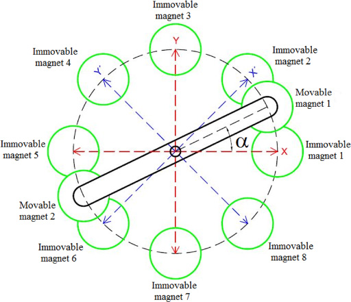
Figure 4 shows a view for the interaction between the two movable magnets and the eight immovable magnets where some of the main variables are described. From Fig. 4, it can be observed that the circle of immovable magnets correspond to 2π, and this circle of immovable magnets is divided in 8 immovable magnets, it yields a factor of $\frac{{\pi}}{4}$ which will be used to get the potential energies.

Fig. 4.

Interaction between the movable magnets and the eight immovable magnets.

Figure 3 and Fig. 4 show the machine. The kinetic energies are explained equal to the past section with the difference that in the past section four immovable magnets were taken into account while in this section eight immovable magnets are take into account. Hence, kinetic energies are equal in both cases because they only depend of the motion produced by the movable magnets 1 and 2, it yields that (8) and (9) are the kinetic energies J ₁ and J ₂.

The potential energies are explained similar to the past section with the difference that in the past section four immovable magnets were taken into account while in this section eight immovable magnets are take into account. Consequently, potential energies of this section are different to the potential energies of the past section because they depend of the interaction produced by the two movable magnets and eight immovable magnets. To obtain the potential energies W ₁ and W ₂, a similar method as the previous is utilized as: $\begin{eqnarray}\displaystyle \text{} & \text{} & \displaystyle W_{1}=\frac{B^{2}}{2{\mu}}V_{11}+\frac{B^{2}}{2{\mu}}V_{12}+\frac{B^{2}}{2{\mu}}V_{13}+\frac{B^{2}}{2{\mu}}V_{14}+\frac{B^{2}}{2{\mu}}V_{15}+\frac{B^{2}}{2{\mu}}V_{16}+\frac{B^{2}}{2{\mu}}V_{17}+\frac{B^{2}}{2{\mu}}V_{18},\end{eqnarray}$ (23) $\begin{eqnarray}\displaystyle \text{} & \text{} & \displaystyle W_{2}=\frac{B^{2}}{2{\mu}}V_{21}+\frac{B^{2}}{2{\mu}}V_{22}+\frac{B^{2}}{2{\mu}}V_{23}+\frac{B^{2}}{2{\mu}}V_{24}+\frac{B^{2}}{2{\mu}}V_{25}+\frac{B^{2}}{2{\mu}}V_{26}+\frac{B^{2}}{2{\mu}}V_{27}+\frac{B^{2}}{2{\mu}}V_{28},\end{eqnarray}$ (24) where from V ₁₁ to V ₁₈ are the volumes of the movable magnet 1 and immovable magnets from 1 to 8, from V ₂₁ to V ₂₈ are the volumes of the movable magnet 2 and immovable magnets from 1 to 8, B is the magnet flux density, and μ is the magnet permeability constant in magnets. From Fig. 3 and Fig. 4, it can be observed that the circle of immovable magnets correspond to 2π, and this circle of immovable magnets is divided in 8 immovable magnets, it yields a factor of $\frac{{\pi}}{4}$ . Then, the same eight parts of the potential energies W ₁ and W ₂ of the before model are obtained plus other eight parts with and angle of ${\alpha}-\frac{{\pi}}{4}$ . Taking it into account, the potential energies W ₁ and W ₂ are: $\begin{eqnarray}\displaystyle W_{1} & = & \displaystyle \frac{B^{2}}{2{\mu}}{\pi}r_{i}^{2}[2r_{g}^{2}(1-\cos {\alpha})+h^{2}]^{0.5}+\frac{B^{2}}{2{\mu}}{\pi}r_{i}^{2}\left[2r_{g}^{2}\left(1-\cos \left({\alpha}-\frac{{\pi}}{4}\right)\right)+h^{2}\right]^{0.5}\nonumber\\ \displaystyle \text{} & \text{} & \displaystyle +∼\frac{B^{2}}{2{\mu}}{\pi}r_{i}^{2}[2r_{g}^{2}(1-\sin {\alpha})+h^{2}]^{0.5}+\frac{B^{2}}{2{\mu}}{\pi}r_{i}^{2}\left[2r_{g}^{2}\left(1-\sin \left({\alpha}-\frac{{\pi}}{4}\right)\right)+h^{2}\right]^{0.5}\nonumber\\ \displaystyle \text{} & \text{} & \displaystyle +\frac{B^{2}}{2{\mu}}{\pi}r_{i}^{2}[2r_{g}^{2}(1+\cos {\alpha})+h^{2}]^{0.5}+\frac{B^{2}}{2{\mu}}{\pi}r_{i}^{2}\left[2r_{g}^{2}\left(1+\cos \left({\alpha}-\frac{{\pi}}{4}\right)\right)+h^{2}\right]^{0.5}\nonumber\\ \displaystyle \text{} & \text{} & \displaystyle +\frac{B^{2}}{2{\mu}}{\pi}r_{i}^{2}[2r_{g}^{2}(1+\sin {\alpha})+h^{2}]^{0.5}+\frac{B^{2}}{2{\mu}}{\pi}r_{i}^{2}\left[2r_{g}^{2}\left(1+\sin \left({\alpha}-\frac{{\pi}}{4}\right)\right)+h^{2}\right]^{0.5}.\end{eqnarray}$ (25) $\begin{eqnarray}\displaystyle W_{2} & = & \displaystyle \frac{B^{2}}{2{\mu}}{\pi}r_{i}^{2}[2r_{g}^{2}(1-\cos {\alpha})+h^{2}]^{0.5}+\frac{B^{2}}{2{\mu}}{\pi}r_{i}^{2}\left[2r_{g}^{2}\left(1-\cos \left({\alpha}-\frac{{\pi}}{4}\right)\right)+h^{2}\right]^{0.5}\nonumber\\ \displaystyle \text{} & \text{} & \displaystyle +∼\frac{B^{2}}{2{\mu}}{\pi}r_{i}^{2}[2r_{g}^{2}(1-\sin {\alpha})+h^{2}]^{0.5}+\frac{B^{2}}{2{\mu}}{\pi}r_{i}^{2}\left[2r_{g}^{2}\left(1-\sin \left({\alpha}-\frac{{\pi}}{4}\right)\right)+h^{2}\right]^{0.5}\nonumber\\ \displaystyle \text{} & \text{} & \displaystyle +\frac{B^{2}}{2{\mu}}{\pi}r_{i}^{2}[2r_{g}^{2}(1+\cos {\alpha})+h^{2}]^{0.5}+\frac{B^{2}}{2{\mu}}{\pi}r_{i}^{2}\left[2r_{g}^{2}\left(1+\cos \left({\alpha}-\frac{{\pi}}{4}\right)\right)+h^{2}\right]^{0.5}\nonumber\\ \displaystyle \text{} & \text{} & \displaystyle +\frac{B^{2}}{2{\mu}}{\pi}r_{i}^{2}[2r_{g}^{2}(1+\sin {\alpha})+h^{2}]^{0.5}+\frac{B^{2}}{2{\mu}}{\pi}r_{i}^{2}\left[2r_{g}^{2}\left(1+\sin \left({\alpha}-\frac{{\pi}}{4}\right)\right)+h^{2}\right]^{0.5}.\end{eqnarray}$ (26) Substituting equations J ₁ of ((8)), J ₂ of ((9)), W ₁ ((25)), and W ₂ of ((26)) in N ₁ and N ₂ of ((1)), Lagrangians N ₁ and N ₂ are: $\begin{eqnarray}\displaystyle N_{1} & = & \displaystyle J_{1}-W_{1}=\left(\frac{1}{24}m_{e1}(a_{1}^{2}+c_{1}^{2})+\frac{1}{2}m_{e1}r_{g}^{2}\right)\dot{{\alpha}}^{2}+\left(\frac{1}{4}m_{i}r_{i}^{2}+\frac{1}{2}m_{i}r_{g}^{2}\right)\dot{{\alpha}}^{2}\nonumber\\ \displaystyle \text{} & \text{} & \displaystyle -∼\frac{B^{2}}{2{\mu}}{\pi}r_{i}^{2}[2r_{g}^{2}(1-\cos {\alpha})+h^{2}]^{0.5}-\frac{B^{2}}{2{\mu}}{\pi}r_{i}^{2}\left[2r_{g}^{2}\left(1-\cos \left({\alpha}-\frac{{\pi}}{4}\right)\right)+h^{2}\right]^{0.5}\nonumber\\ \displaystyle \text{} & \text{} & \displaystyle -∼\frac{B^{2}}{2{\mu}}{\pi}r_{i}^{2}[2r_{g}^{2}(1-\sin {\alpha})+h^{2}]^{0.5}-\frac{B^{2}}{2{\mu}}{\pi}r_{i}^{2}\left[2r_{g}^{2}\left(1-\sin \left({\alpha}-\frac{{\pi}}{4}\right)\right)+h^{2}\right]^{0.5}\nonumber\\ \displaystyle \text{} & \text{} & \displaystyle -∼\frac{B^{2}}{2{\mu}}{\pi}r_{i}^{2}[2r_{g}^{2}(1+\cos {\alpha})+h^{2}]^{0.5}-\frac{B^{2}}{2{\mu}}{\pi}r_{i}^{2}\left[2r_{g}^{2}\left(1+\cos \left({\alpha}-\frac{{\pi}}{4}\right)\right)+h^{2}\right]^{0.5}\nonumber\\ \displaystyle \text{} & \text{} & \displaystyle -∼\frac{B^{2}}{2{\mu}}{\pi}r_{i}^{2}[2r_{g}^{2}(1+\sin {\alpha})+h^{2}]^{0.5}-\frac{B^{2}}{2{\mu}}{\pi}r_{i}^{2}\left[2r_{g}^{2}\left(1+\sin \left({\alpha}-\frac{{\pi}}{4}\right)\right)+h^{2}\right]^{0.5}.\end{eqnarray}$ (27) $\begin{eqnarray}\displaystyle N_{2} & = & \displaystyle J_{2}-W_{2}=\left(\frac{1}{24}m_{e2}(a_{2}^{2}+c_{2}^{2})+\frac{1}{2}m_{e2}r_{g}^{2}\right)\dot{{\alpha}}^{2}+\left(\frac{1}{4}m_{i}r_{i}^{2}+\frac{1}{2}m_{i}r_{g}^{2}\right)\dot{{\alpha}}^{2}\nonumber\\ \displaystyle \text{} & \text{} & \displaystyle -∼\frac{B^{2}}{2{\mu}}{\pi}r_{i}^{2}[2r_{g}^{2}(1-\cos {\alpha})+h^{2}]^{0.5}-\frac{B^{2}}{2{\mu}}{\pi}r_{i}^{2}\left[2r_{g}^{2}\left(1-\cos \left({\alpha}-\frac{{\pi}}{4}\right)\right)+h^{2}\right]^{0.5}\nonumber\\ \displaystyle \text{} & \text{} & \displaystyle -∼\frac{B^{2}}{2{\mu}}{\pi}r_{i}^{2}[2r_{g}^{2}(1-\sin {\alpha})+h^{2}]^{0.5}-\frac{B^{2}}{2{\mu}}{\pi}r_{i}^{2}\left[2r_{g}^{2}\left(1-\sin \left({\alpha}-\frac{{\pi}}{4}\right)\right)+h^{2}\right]^{0.5}\nonumber\\ \displaystyle \text{} & \text{} & \displaystyle -∼\frac{B^{2}}{2{\mu}}{\pi}r_{i}^{2}[2r_{g}^{2}(1+\cos {\alpha})+h^{2}]^{0.5}-\frac{B^{2}}{2{\mu}}{\pi}r_{i}^{2}\left[2r_{g}^{2}\left(1+\cos \left({\alpha}-\frac{{\pi}}{4}\right)\right)+h^{2}\right]^{0.5}\nonumber\\ \displaystyle \text{} & \text{} & \displaystyle -∼\frac{B^{2}}{2{\mu}}{\pi}r_{i}^{2}[2r_{g}^{2}(1+\sin {\alpha})+h^{2}]^{0.5}-\frac{B^{2}}{2{\mu}}{\pi}r_{i}^{2}\left[2r_{g}^{2}\left(1+\sin \left({\alpha}-\frac{{\pi}}{4}\right)\right)+h^{2}\right]^{0.5}.\end{eqnarray}$ (28) Substituting N ₁ of ((27)) and N ₂ of ((28)) into ((1)) yields the torque of magnets τ as: $\begin{eqnarray} \displaystyle {\tau} & = & \displaystyle \left(\frac{1}{12}m_{e1}(a_{1}^{2}+c_{1}^{2})+m_{e1}r_{g}^{2}\right)\ddot{{\alpha}}+\left(\frac{1}{2}m_{i}r_{i}^{2}+m_{i}r_{g}^{2}\right)\ddot{{\alpha}}\nonumber\\ \displaystyle \text{} & \text{} & \displaystyle +∼\frac{{\pi}B^{2}r_{g}^{2}r_{i}^{2}\sin {\alpha}}{2{\mu}[h^{2}+2r_{g}^{2}(1-\cos {\alpha})]^{0.5}}+\frac{{\pi}B^{2}r_{g}^{2}r_{i}^{2}\sin \left({\alpha}-{\displaystyle \frac{{\pi}}{4}}\right)}{2{\mu}\left[h^{2}+2r_{g}^{2}\left(1-\cos \left({\alpha}-{\displaystyle \frac{{\pi}}{4}}\right)\right)\right]^{0.5}}\nonumber\\ \displaystyle \text{} & \text{} & \displaystyle -∼{\displaystyle \frac{{\pi}B^{2}r_{g}^{2}r_{i}^{2}\cos {\alpha}}{2{\mu}[h^{2}+2r_{g}^{2}(1-\sin {\alpha})]^{0.5}}}-{\displaystyle \frac{{\pi}B^{2}r_{g}^{2}r_{i}^{2}\cos \left({\alpha}-{\displaystyle \frac{{\pi}}{4}}\right)}{2{\mu}\left[h^{2}+2r_{g}^{2}\left(1-\sin \left({\alpha}-{\displaystyle \frac{{\pi}}{4}}\right)\right)\right]^{0.5}}}\nonumber\\ \displaystyle \text{} & \text{} & \displaystyle -∼{\displaystyle \frac{{\pi}B^{2}r_{g}^{2}r_{i}^{2}\sin {\alpha}}{2{\mu}[h^{2}+2r_{g}^{2}(1+\cos {\alpha})]^{0.5}}}-{\displaystyle \frac{{\pi}B^{2}r_{g}^{2}r_{i}^{2}\sin \left({\alpha}-{\displaystyle \frac{{\pi}}{4}}\right)}{2{\mu}\left[h^{2}+2r_{g}^{2}\left(1+\cos \left({\alpha}-{\displaystyle \frac{{\pi}}{4}}\right)\right)\right]^{0.5}}}\nonumber\\ \displaystyle \text{} & \text{} & \displaystyle +∼{\displaystyle \frac{{\pi}B^{2}r_{g}^{2}r_{i}^{2}\cos {\alpha}}{2{\mu}[h^{2}+2r_{g}^{2}(1+\sin {\alpha})]^{0.5}}}+{\displaystyle \frac{{\pi}B^{2}r_{g}^{2}r_{i}^{2}\cos \left({\alpha}-{\displaystyle \frac{{\pi}}{4}}\right)}{2{\mu}\left[h^{2}+2r_{g}^{2}\left(1+\sin \left({\alpha}-{\displaystyle \frac{{\pi}}{4}}\right)\right)\right]^{0.5}}}\nonumber\\ \displaystyle \text{} & \text{} & \displaystyle +∼\left({\displaystyle \frac{1}{24}}m_{e2}(a_{2}^{2}+c_{2}^{2})+{\displaystyle \frac{1}{2}}m_{e2}r_{g}^{2}\right)\dot{{\alpha}}^{2}+\left({\displaystyle \frac{1}{4}}m_{i}r_{i}^{2}+{\displaystyle \frac{1}{2}}m_{i}r_{g}^{2}\right)\dot{{\alpha}}^{2}+b\dot{{\alpha}}\nonumber\\ \displaystyle \text{} & \text{} & \displaystyle -∼{\displaystyle \frac{{\pi}B^{2}r_{g}^{2}r_{i}^{2}\sin {\alpha}}{2{\mu}[h^{2}+2r_{g}^{2}(1+\cos {\alpha})]^{0.5}}}-{\displaystyle \frac{{\pi}B^{2}r_{g}^{2}r_{i}^{2}\sin \left({\alpha}-{\displaystyle \frac{{\pi}}{4}}\right)}{2{\mu}\left[h^{2}+2r_{g}^{2}\left(1+\cos \left({\alpha}-{\displaystyle \frac{{\pi}}{4}}\right)\right)\right]^{0.5}}}\nonumber\\ \displaystyle \text{} & \text{} & \displaystyle +∼{\displaystyle \frac{{\pi}B^{2}r_{g}^{2}r_{i}^{2}\cos {\alpha}}{2{\mu}[h^{2}+2r_{g}^{2}(1+\sin {\alpha})]^{0.5}}}+{\displaystyle \frac{{\pi}B^{2}r_{g}^{2}r_{i}^{2}\cos \left({\alpha}-{\displaystyle \frac{{\pi}}{4}}\right)}{2{\mu}\left[h^{2}+2r_{g}^{2}\left(1+\sin \left({\alpha}-{\displaystyle \frac{{\pi}}{4}}\right)\right)\right]^{0.5}}}\nonumber\\ \displaystyle \text{} & \text{} & \displaystyle +∼{\displaystyle \frac{{\pi}B^{2}r_{g}^{2}r_{i}^{2}\sin {\alpha}}{2{\mu}[h^{2}+2r_{g}^{2}(1-\cos {\alpha})]^{0.5}}}+{\displaystyle \frac{{\pi}B^{2}r_{g}^{2}r_{i}^{2}\sin \left({\alpha}-{\displaystyle \frac{{\pi}}{4}}\right)}{2{\mu}\left[h^{2}+2r_{g}^{2}\left(1-\cos \left({\alpha}-{\displaystyle \frac{{\pi}}{4}}\right)\right)\right]^{0.5}}}\nonumber\\ \displaystyle \text{} & \text{} & \displaystyle -∼{\displaystyle \frac{{\pi}B^{2}r_{g}^{2}r_{i}^{2}\cos {\alpha}}{2{\mu}[h^{2}+2r_{g}^{2}(1-\sin {\alpha})]^{0.5}}}-{\displaystyle \frac{{\pi}B^{2}r_{g}^{2}r_{i}^{2}\cos \left({\alpha}-{\displaystyle \frac{{\pi}}{4}}\right)}{2{\mu}\left[h^{2}+2r_{g}^{2}\left(1-\sin \left({\alpha}-{\displaystyle \frac{{\pi}}{4}}\right)\right)\right]^{0.5}}}. \end{eqnarray}$ (29)

4.2. The electric model

The electric model is explained equal to the past section with the difference that in the past section four immovable magnets were taken into account while in this section eight immovable magnets are take into account. The electric model is equal in both cases because it only depends of the motion produced by the two movable magnets, it yields that (21) is the electric model.

4.3. The mathematical model in state space

Thus, (29) is the conversion between the magnetism and mechanic motions, and (21) is the conversion between the mechanic motions and electricity, they are known as the mathematical model of the machine. States are selected as z ₁ = i, z ₂ = 𝛼, $z_{3}=\dot{{\alpha}}$ and the input is selected as v = τ. Finally, the mathematical model of equations (29) and (21) represents the machine of eight immovable magnets and two movable magnets as: $\begin{eqnarray}\displaystyle \text{} & \text{} & \displaystyle {\dot{z}}_{1}=-{\displaystyle \frac{(R+R_{e})}{L}}z_{1}+{\displaystyle \frac{K_{m}}{L}}z_{3},\nonumber\\ \displaystyle \text{} & \text{} & \displaystyle {\dot{z}}_{2}=z_{3},\nonumber\end{eqnarray}$ $\begin{eqnarray}\displaystyle {\dot{z}}_{3} & = & \displaystyle \left({\displaystyle \frac{1}{m_{e}\left({\displaystyle \frac{1}{24}}a^{2}+{\displaystyle \frac{1}{24}}c^{2}+r_{g}^{2}\right)+m_{i}(r_{i}^{2}+2r_{g}^{2})}}\right)\nonumber\\ \displaystyle \text{} & \text{} & \displaystyle \ast \left(v-{\displaystyle \frac{{\pi}B^{2}r_{i}^{2}r_{g}^{2}\sin z_{2}}{{\mu}[h^{2}+2r_{g}^{2}(1-\cos z_{2})]^{0.5}}}-{\displaystyle \frac{{\pi}B^{2}r_{i}^{2}r_{g}^{2}\sin \left(z_{2}-{\displaystyle \frac{{\pi}}{4}}\right)}{{\mu}\left[h^{2}+2r_{g}^{2}\left(1-\cos \left(z_{2}-{\displaystyle \frac{{\pi}}{4}}\right)\right)\right]^{0.5}}}\right.\nonumber\\ \displaystyle \text{} & \text{} & \displaystyle -∼{\displaystyle \frac{{\pi}B^{2}r_{i}^{2}r_{g}^{2}\cos z_{2}}{{\mu}[h^{2}+2r_{g}^{2}(1+\sin z_{2})]^{0.5}}}-{\displaystyle \frac{{\pi}B^{2}r_{i}^{2}r_{g}^{2}\cos z_{2}}{{\mu}\left[h^{2}+2r_{g}^{2}\left(1+\sin \left(z_{2}-{\displaystyle \frac{{\pi}}{4}}\right)\right)\right]^{0.5}}}\nonumber\\ \displaystyle \text{} & \text{} & \displaystyle +∼{\displaystyle \frac{{\pi}B^{2}r_{i}^{2}r_{g}^{2}\sin z_{2}}{{\mu}[h^{2}+2r_{g}^{2}(1+\cos z_{2})]^{0.5}}}+{\displaystyle \frac{{\pi}B^{2}r_{i}^{2}r_{g}^{2}\sin \left(z_{2}-{\displaystyle \frac{{\pi}}{4}}\right)}{{\mu}\left[h^{2}+2r_{g}^{2}\left(1+\cos \left(z_{2}-{\displaystyle \frac{{\pi}}{4}}\right)\right)\right]^{0.5}}}\nonumber\\ \displaystyle \text{} & \text{} & \displaystyle +∼\left.{\displaystyle \frac{{\pi}B^{2}r_{i}^{2}r_{g}^{2}\cos z_{2}}{{\mu}[h^{2}+2r_{g}^{2}(1-\sin z_{2})]^{0.5}}}+{\displaystyle \frac{{\pi}B^{2}r_{i}^{2}r_{g}^{2}\cos \left(z_{2}-{\displaystyle \frac{{\pi}}{4}}\right)}{{\mu}\left[h^{2}+2r_{g}^{2}\left(1-\sin \left(z_{2}-{\displaystyle \frac{{\pi}}{4}}\right)\right)\right]^{0.5}}}-bz_{3}\right).\end{eqnarray}$ (30)

5. Experiments

In this section, the machine with two immovable magnets and two movable magnets of [21,22], the machine of four immovable magnets and two movable magnets of (22), and the machine of eight immovable magnets and two movable magnets of (30) present the comparison between experiments and simulations for one input. In this section, the machine with two immovable magnets and two movable magnets of [21,22] is called 2ImmovableMagnets, the machine of four immovable magnets and two movable magnets of (22) is called 4ImmovableMagnets, and the machine of eight immovable magnets and two movable magnets of (30) is called 8ImmovableMagnets.

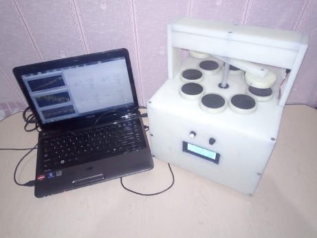
Figure 5 shows the prototype employed to perform each experiment. This prototype is transformed to represent each of the machines 2ImmovableMagnets, 4ImmovableMagnets, or 8ImmovableMagnets.

The first purpose of this article is to validate the three mathematical models of machines based on obtaining that the experiments are near to simulations. If this is complied, the mathematical models of all machines really represent the real prototype.

The second purpose of this article is to observe which of the proposed machines 2ImmovableMagnets, 4ImmovableMagnets, or 8ImmovableMagnets creates more electricity.

For Simulation of all machines, parameter values for mathematical models are shown in the Table 1.

5.1. Validation of the mathematical models

In this sub-section, the first purpose of this article is to validate the three mathematical models of machines based on obtaining that the experiments are near to simulations, if this is complied, the mathematical models of all machines really represent the real prototype, and the root mean square error (MSE) will be used in comparisons, it is: $\begin{eqnarray}\displaystyle MSE=\left({\displaystyle \frac{1}{T}}\int _{0}^{T}z_{k}^{2}d{\tau}\right)^{\frac{1}{2}}, & & \displaystyle\end{eqnarray}$ (31)

$z_{1}^{2}=(z_{1}-z_{1r})^{2}$ for state 1, $z_{2}^{2}=(z_{2}-z_{2r})^{2}$ for state 2, $z_{3}^{2}=(z_{3}-z_{3r})^{2}$ for state 3 in all machines, z ₁, z ₂, z ₃ are for the simulations and z _1r, z _2r, z _3r are for the experiments, T is the final time.

Fig. 5.

Prototype of the machine.

Table 1

Parameters of machines

Parameter	Value
m _i	9.2 × 10⁻² kg
μ	9.42 × 10⁻⁵ Hm⁻¹
B	8.4 × 10⁻¹ T
L	6.03 × 10⁻¹ H
K _m	45 × 10⁻² Vsrad⁻¹
b	1 × 10⁻¹ kgm² rads⁻¹
m _e	5 × 10⁻³ kg
h	4 × 10⁻² m
R	6.96 Ω
R _e	30 Ω
r _g	7.5 × 10⁻² m
r _i	2.9 × 10⁻² m
a	1.5 × 10⁻¹ m
c	1.5 × 10⁻² m

Figure 6 shows the comparisons between experiments and simulations for input and states of the machine 2ImmovableMagnets for a time from 0 s to 2 s. Table 2 shows the MSE of (31).

Fig. 6.

Comparison between experiments and simulations for 2ImmovableMagnets.

Table 2

MSE for 2ImmovableMagnets

Machines	2ImmovableMagnets
MSE for v	2.6456
MSE for z ₁	0.0886
MSE for z ₂	3.0214
MSE for z ₃	6.7950

Figure 7 shows the comparisons between experiments and simulations for input and states of the machine 4ImmovableMagnets for a time from 0 s to 2 s. Table 3 shows the MSE of (31).

Fig. 7.

Comparison between experiments and simulations for 4ImmovableMagnets.

Table 3

MSE for 4ImmovableMagnets

Machines	2ImmovableMagnets
MSE for v	2.3891
MSE for z ₁	0.0796
MSE for z ₂	3.5020
MSE for z ₃	7.9843

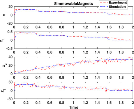
Figure 8 shows the comparisons between experiments and simulations for input and states of the machine 8ImmovableMagnets for a time from 0 s to 2 s. Table 4 shows the MSE of (31).

Fig. 8.

Comparison between experiments and simulations for 8ImmovableMagnets.

Table 4

MSE for 8ImmovableMagnets

Machines	2ImmovableMagnets
MSE for v	2.4092
MSE for z ₁	0.0803
MSE for z ₂	2.5683
MSE for z ₃	7.5934

From Fig. 6, Fig. 7, and Fig. 8, it is observed that the first purpose of this article is complied because for the three kinds of machines the experiments are near to simulations. From Table 2, Table 3, and Table 4, it is observed that the first purpose of this article is complied because for the three kinds of proposed machines the MSE is small. Then, the proposed mathematical models of all machines are validated because they really represent the prototype.

5.2. Comparison of the mathematical models

In this sub-section, the second purpose of this article is to observe which of the proposed machines 2ImmovableMagnets, 4ImmovableMagnets, or 8ImmovableMagnets creates more electricity, and the root mean square error (MSE) will be used in comparisons, it is: $\begin{eqnarray}\displaystyle MSE=\left({\displaystyle \frac{1}{T}}\int _{0}^{T}z_{k}^{2}d{\tau}\right)^{\frac{1}{2}}, & & \displaystyle\end{eqnarray}$ (32)

$z_{1}^{2}=(z_{1})^{2}$ for state 1, $z_{2}^{2}=(z_{2})^{2}$ for state 2, $z_{3}^{2}=(z_{3})^{2}$ for state 3 in all machines, z ₁, z ₂, z ₃ are for the simulations, T is the final time.

In the first simulation the input v = 1 for t = [0, 5] s and v = 0 for t = [5, 10] s is utilized for all machines. Figure 9 shows inputs and states of all machines for a time from 0 s to 10 s. Table 2 shows the MSE of (32).

Fig. 9.

Inputs and states of all machines for the first simulation.

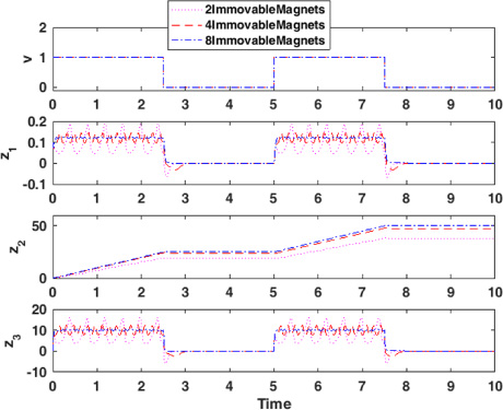
In the second simulation the input v = 1 for t = [0, 2.5] s and t = [5, 7.5] s, and v = 0 for t = [2.5, 5] s and t = [7.5, 10] s is utilized for all machines: Fig. 10 shows inputs and states of all machines for a time from 0 s to 10 s. Table 3 shows the MSE of (32).

Fig. 10.

Inputs and states of all machines for the second simulation.

From Fig. 9 and Fig. 10, it is observed that the 8ImmovableMagnets presents the creation of more electricity than both 4ImmovableMagnets and 2ImmovableMagnets because for the same values of v the machine 8ImmovableMagnets presents higher values for z ₂. From Table 5 and Table 6, it can be observed that 8ImmovableMagnets reaches better results than both 4ImmovableMagnets and 2ImmovableMagnets because the MSE for the 8ImmovableMagnets is bigger than for 4ImmovableMagnets and 2ImmovableMagnets. Then, the 8ImmovableMagnets obtains the second purpose of this article, the creation of more electricity.

Table 5

MSE for the first simulation

Generators	MSE z ₁	MSE z ₂	MSE z ₃
2ImmovableMagnets	0.0531	21.9468	4.4019
4ImmovableMagnets	0.0597	28.0838	4.9248
8ImmovableMagnets	0.0608	28.9676	4.9931

Table 6

MSE for the second simulation

Generators	MSE z ₁	MSE z ₂	MSE z ₃
2ImmovableMagnets	0.0531	18.4762	4.4076
4ImmovableMagnets	0.0595	23.1573	4.9114
8ImmovableMagnets	0.0607	24.5505	4.9872

6. Conclusions

In this article, the mathematical model of a machine with eight immovable magnets and two movable magnets, and the mathematical model of a machine with four immovable magnets and two movable magnets were proposed. The proposed mathematical models were validated based on experiments with a prototype. The introduced machines were compared with the machine with two immovable magnets and two movable magnets producing that the introduced machines reached better performance in comparison with the other machine because the designed machines create more electricity. The suggested machines could be applied as a fuel for several kind of mechanic processes. In the future, other kind of machines will be studied, or the discussed machines will be applied in a mechanic process.

Footnotes

Acknowledgements

Authors thank to editors and reviewers for valuable comments of this research. Authors thank the IPN, CONACYT, SIP, and COFAA for their support.

References

Chen

and Du

, Model of ferromagnetic steels for lightning transient analysis, IET Science, Measurement & Technology 12(3) (2018), 301–307.

Xie

Chen

Uchimoto

and Takagi

, A fast forward simulation scheme for eddy current testing of crack in a structure of carbon fiber reinforced polymer laminate, IEEE Access 7 (2019), 152278–152288.

Gong

Kim

and Kim

, Magnetism in 𝛼-RuCl: Dependence on Coulomb interaction and Hund’s coupling, Journal of the Korean Physical Society 73(11) (2018), 1691–1697.

Lee

J.W.

Song

M.S.

Cho

K.K.

Cho

B.K.

and Nam

, Magnetocaloric properties of AlFe B including paramagnetic impurities of Al Fe, Journal of the Korean Physical Society 73(10) (2018), 1555–1560.

Qian

H.D.

P.Z.

Lim

J.T.

Kim

J.W.

and Park

, Magnetic properties of Mn Al C /Sm Fe N and Mn Al C /Fe Co composites, Journal of the Korean Physical Society 73(11) (2018), 1703–1707.

Nakai

, Magnetic domain transition controlled by distributed normal magnetic field for stepped magneto-impedance sensor, International Journal of Applied Electromagnetics and Mechanics 59(1) (2019), 105–114.

Park

J.K.

Lee

K.W.

Choi

D.M.

and Lee

C.E.

, Electron paramagnetic resonance study of Al-incorporated ZnO:Mn diluted magnetic semiconductors, Journal of the Korean Physical Society 73(12) (2018), 1884–1888.

Sun

Urayama

Hashimoto

Kojima

Uchimoto

and Takagi

, Novel electromagnetic acoustic transducer for measuring the thickness of small specimen areas, International Journal of Applied Electromagnetics and Mechanics 59(4) (2019), 1495–1504.

Xie

Cai

Chen

H.-E.

Zhou

Chen

Uchimoto

and Takagi

, A simulation method to evaluate electrical conductivity of closed-cell aluminum foam, International Journal of Applied Electromagnetics and Mechanics 58(3) (2018), 289–307.

10.

Yang

C.H.

Song

Jhun

Hwang

W.S.

Hong

S.D.

Woo

S.B.

Sung

T.H.

Jeong

S.W.

and Yoo

H.H.

, A high efficient piezoelectric windmill using magnetic force for low wind speed in wireless sensor networks, Journal of the Korean Physical Society 73(12) (2018), 1889–1894.

11.

Wang

and Li

, Analysis and experimental research on air gap characteristics of permanent magnet low resistance belt conveyor, IET Science, Measurement & Technology 12(4) (2018), 472–478.

12.

Xiao

Duan

and Shi

, A novel feature extraction method of direction navigability analysis for geomagnetic navigation, Journal of Computational Methods in Sciences and Engineering 18(1) (2018), 47–59.

13.

Qian

Bao

and Wu

, Magnetic field modeling and analysis for permanent magnet synchronous linear motors, International Journal of Applied Electromagnetics and Mechanics 60(2) (2019), 209–221.

14.

Sheng

Geng

Zhang

Yang

Xia

and Cheng

, Testing of a 100 kW oil-free high-speed permanent-magnet synchronous motor, International Journal of Applied Electromagnetics and Mechanics 59(2) (2019), 775–783.

15.

Ishikawa

Watanabe

and Suzuki

, Proposal of a permanent magnet synchronous machine with asymmetrical rotor, International Journal of Applied Electromagnetics and Mechanics 59(3) (2019), 797–804.

16.

Jin

Sun

Yang

Wang

Chen

and Li

, A novel four degree-of-freedoms bearingless permanent magnet machine using modified cross feedback control scheme for flywheel energy storage systems, International Journal of Applied Electromagnetics and Mechanics 60(3) (2019), 379–392.

17.

Shi

Zhang

Guo

Wang

and Xia

, Optimal designing of rotor geometry in interior permanent magnet machine to broaden speed range, International Journal of Applied Electromagnetics and Mechanics 60(3) (2019), 337–353.

18.

Vertesy

Tomas

Skrbek

Uchimoto

and Takagi

, Investigation of cast iron matrix constituents by magnetic adaptive testing, IEEE Transactions on Magnetics 55(3) (2019), 6200306.

19.

Xie

Tong

Chen

H.E.

Chen

Uchimoto

and Takagi

, Influence of plastic deformation and fatigue damage on electromagnetic properties of 304 austenitic stainless steel, IEEE Transactions on Magnetics 54(8) (2018), 6201710.

20.

Han

and Chu

, A general electromagnetic excitation model for electrical machines considering the magnetic saturation and rub impact, Journal of Sound and Vibration 416 (2018), 154–171.

21.

Rubio

J.J.

Pieper

Meda-Campaña

J.A.

Aguilar

Rangel

V.I.

and Gutierrez

G.J.

, Modeling and regulation of two mechanical systems, IET Science, Measurement & Technology 12(5) (2018), 657–665.

22.

Rubio

J.J.

Aguilar

Meda-Campaña

J.A.

Ochoa

Balcazar

and Lopez

, An electricity generator based on the interaction of static and dynamic magnets, IEEE Transactions on Magnetics 55(8) (2019), 8204511.