Influence of the magnetization vector misalignment on the magnetic force of permanent ring magnet and soft magnetic cylinder

Abstract

The aim of this paper is to emphasize the influence of the magnetization vector misalignment to the magnetic force. In this concrete example the force between permanent ring magnet and soft magnetic cylinder was analyzed. Configuration that can be seen in different devices that incorporate permanent magnets.

Magnetic force between permanent ring magnet and soft magnetic cylinder is calculated using hybrid boundary element method and semi-analytical approach based on fictitious magnetization charges. By selecting the angle of the magnetization vector inclination, obtained expression can be used for the force calculation of axially or radially magnetized permanent magnet and magnetic body of finite dimension.

Keywords

Hybrid boundary element method (HBEM)magnetization charges magnetic force permanent ring magnet

1. Introduction

Permanent magnets are increasingly being used as a result of the wider adoption of electrical devices and gadgets. There is a constant need for their optimization and size reduction, which leads to new mathematical methods for their field calculation. The quality of electrical devices that contain permanent magnets is dependent on the magnetic material they are made of, their magnetization, as well as their size.

Nowadays, permanent magnets have become preferable choice (due to their low cost) in different applications since they do not require separate power supply. The most common ones being magnetic couplings and bearings, magnetic assemblies, sensors, motors, and actuators. They have also “infiltrated” the design of various medical and mission critical systems. Main application is in the field of actuation, localization, screening, and drug delivery.

Since Yonnet presented the first study concerning different permanent magnet configuration [1], many scientists around the World are dealing with this issue by carrying out various researches in order to determine the magnetic field of permanent magnets and the force between them accurately and efficiently [2–4]. Many different methods for permanent magnet field calculation are available, aiming towards the simplest and fastest analysis of magnetic structures in relation to different parameters. In most cases, analytical methods for permanent magnet field calculation based on the distribution of magnetic charges or Ampere’s microscopic currents are limited to block and cylindrical structures [5,6]. In order to overcome drawbacks of analytical and numerical methods, numerous semi-numerical approaches were proposed by different authors [7–9].

A special group of problems was addressed, considering permanent magnet structures in the vicinity of different bodies with magnetic material composition. In the survey of existing literature, in most of the cases, only the field or force between permanent magnet and infinite magnetic plain calculation was available [10]. Problems of this kind were solved by first applying the method of images, after which Ampere’s approach [11,12] or Coulombian approach [13] was used to model the configuration. This paper presents modeling of permanent magnet in the vicinity of a body of finite dimensions made of soft magnetic material.

Each modeling technique is based on certain assumptions that, in the end, introduce errors in the results obtained. Besides, the manufacturing process of any permanent magnet-based device is influenced by different inaccuracies. The most common performance degradation causes are misalignment of the magnetization angle, variations in remanent flux density and relative permeability.

Permanent magnets can be magnetized using large magnetizing coils. If the magnetic axis of permanent magnet domains is not precisely aligned with the geometrical axis of the permanent magnet, the resulting magnetization will exhibit a small inclination with respect to the geometry. The reason lies in the fact that the magnetizing coil magnetic field is not totally uniform. In order to model magnetization vector misalignment and to estimate the influence that it has on the magnetic force, “homebrew” hybrid boundary element method (HBEM), described in the paper, is used along with semi-analytical approach based on fictitious magnetization charges and discretization technique. Hybrid boundary element method (HBEM) was developed at the Department of Theoretical Electrical Engineering, Faculty of Electronic Engineering of Niš, and was successfully used for the analysis of multilayered electromagnetic problems [14–16]. Magnetization vector misalignment influence on the magnetic force between ring permanent magnet and soft magnetic cylinder is analyzed in the paper. The results presented are important in the modeling process itself and in the manufacturing process of various devices that incorporate permanent magnets.

2. Model description and force calculation

Magnetic assemblies are elements made of different housings and permanent magnets. That way the magnetic circuits are altered so specific magnetic characteristics can be achieved, and its durability extended. Case considered in this paper can help in the process of magnetic assembly design.

Mass production of different assemblies and permanent magnets in general, leads to design errors which are usually detected in the final stages of the manufacturing process. Methodology presented allows faster analysis of the magnetic force variation with parametric change (having either radial or axial magnetization). Also, this approach allows influence analysis of the magnetization vector misalignment to the magnetic force, depending on system parameters (magnet size, cylinder size, magnetic permeability).

A permanent ring magnet positioned above the cylinder made of linear magnetic material with relative permeability μ_r2, is considered. Presumption is that there is a misalignment in the axial magnetization of the permanent magnet as it is shown in the Fig. 1.

Fig. 1.

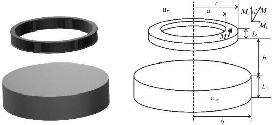
Ring permanent magnet positioned above magnetic cylinder.

Fig. 2.

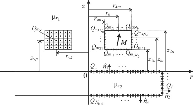
Discretization model.

In order to calculate the magnetic force, the approach based on fictitious magnetization charges and discretization technique is used, along with the hybrid boundary element method.

Considering a misalignment in magnetization vector (Fig. 1), there are axial ( M _z) and radial ( M _r) magnetization vector components, $\begin{eqnarray}\displaystyle \boldsymbol{M}=\boldsymbol{M}_{r}+\boldsymbol{M}_{z}=M\sin {\alpha}\cdot \hat{r}+M\cos {\alpha}\cdot \hat{z}. & & \displaystyle\end{eqnarray}$ (1)

Since there is a magnetization vector component in the axial direction, the fictitious magnetic charges exist on the bottom and the top bases of the magnet, ${\eta}_{m}=\hat{n}\cdot M_{z}$ .

On the other hand, because of the radial magnetization vector component, there are surface magnetization charges on the ring magnet’s covers ( ${\eta}_{mc}=\hat{n}\cdot M_{r}$ ) and also volume charges inside the magnet (𝜌_m = −𝛻⋅ M = −M _r∕r) [17]. Therefore, in case when the magnetization vector misalignment exists, the permanent ring magnet’s covers, bases and volume can be discretized into system of circular loops, loaded with different magnetic charges (Fig. 2).

As well, the cylinder is made of linear magnetic material with permeability μ_r2 and the influence of the magnetic material can be replaced with the system composed of toroidal magnetic sources placed on the boundary surface of two different materials (on the magnetic cylinder cover and bases) [18].

To calculate the magnetic force that exists between ring permanent magnet and soft magnetic cylinder, permanent magnet and magnetic cylinder are discretized and considered as a system of circular loops and thin toroidal magnetic sources. Discretization model and distributions of permanent ring magnet’s magnetic charges along with toroidal sources are presented in the Fig. 2. The superposition of results obtained for the magnetic force between two circular loops is used. The axial magnetic force between two circular loops loaded with different magnetic charges is derived in [17].

Magnetic scalar potential of the considered system is $\begin{eqnarray} \displaystyle \displaystyle {\varphi}_{m}\text{} & =\text{} & \displaystyle {\displaystyle \frac{1}{2{\pi}^{2}}}\Big(S(Q_{m1},r,r_{n},z,z_{1n},n,N_{b})+S(Q_{m2},r,r_{n},z,z_{2n},n,N_{b})\nonumber\\ \displaystyle \displaystyle \text{} & \text{} & \displaystyle \quad +∼S(Q_{m3},r,r_{3m},z,z_{m},m,N_{c})+S(Q_{m4},r,r_{4m},z,z_{m},m,N_{c})\nonumber\\ \displaystyle \displaystyle \text{} & \text{} & \displaystyle \quad +∼\mathop{\sum }_{p=1}^{N_{v1}}S(Q_{mv},r,r_{vk},z,z_{vp},k,N_{v2})+S(Q_{i},r,r_{i},z,z_{i},i,N_{\text{tot}})\Big) \end{eqnarray}$ (2) where $\begin{eqnarray}\displaystyle \text{} & \text{}S(Q,r,r_{0},z,z_{0},n,N)=\mathop{\sum }_{n=1}^{N}Q{\displaystyle \frac{K(r,r_{0},z,z_{0})}{\sqrt{(r+r_{0})^{2}+(z-z_{0})^{2}}}}, & \displaystyle \nonumber\\ \displaystyle \text{} & \text{}K(r,r_{0},z,z_{0})=K\left({\displaystyle \frac{{\pi}}{2}},{\displaystyle \frac{4rr_{0}}{(r+r_{0})^{2}+(z-z_{0})^{2}}}\right). & \displaystyle \nonumber\end{eqnarray}$ Parameters of permanent magnet bases (Fig. 2) are $\begin{eqnarray}\displaystyle \displaystyle \text{} & \text{}r_{n}=a+{\displaystyle \frac{2n-1}{2N_{b}}}(c-a),\quad n=1,2,\ldots ,N_{b} & \displaystyle \nonumber\\ \displaystyle \displaystyle \text{} & \text{}z_{1n}=h,\quad z_{2n}=h+L_{1}, & \displaystyle\end{eqnarray}$ (3) while the magnetic charges of lower and upper bases are $\begin{eqnarray}\displaystyle \text{} & \text{}Q_{m1}=Q_{m1n}=-M_{z}2{\pi}r_{n}{\displaystyle \frac{c-a}{N_{b}}},\quad n=1,2,\ldots ,N_{b}, & \displaystyle\end{eqnarray}$ (4) $\begin{eqnarray}\displaystyle \text{} & \text{}Q_{m2}=Q_{m2n}=M_{z}2{\pi}r_{n}{\displaystyle \frac{c-a}{N_{b}}},\quad n=1,2,\ldots ,N_{b}. & \displaystyle\end{eqnarray}$ (5) N _b is the number of discretization segments (circular loops) of each permanent magnet’s base.

Parameters of permanent magnet cover segments are $\begin{eqnarray}\displaystyle \text{} & \text{}r_{3m}=a,\quad r_{4m}=c, & \displaystyle \nonumber\\ \displaystyle \displaystyle \text{} & \text{}z_{m}=h+{\displaystyle \frac{2m-1}{2N_{c}}}L_{1},\quad m=1,2\ldots ,N_{c} & \displaystyle\end{eqnarray}$ (6) and magnetic charges of inner and outer covers are $\begin{eqnarray}\displaystyle \text{} & \text{}Q_{m3}=Q_{m3m}=-M_{r}2{\pi}a{\displaystyle \frac{L_{1}}{N_{c}}},\quad m=1,2,\ldots ,N_{c}, & \displaystyle\end{eqnarray}$ (7) $\begin{eqnarray}\displaystyle \text{} & \text{}Q_{m4}=Q_{m4m}=M_{r}2{\pi}c{\displaystyle \frac{L_{1}}{N_{c}}},\quad m=1,2,\ldots ,N_{c}. & \displaystyle\end{eqnarray}$ (8) N _c is the number of cover segments.

N _b and N _c are calculated from the initial number of surface segments, N _s, and they depend on the permanent magnet dimensions.

Fig. 3.

Distribution of magnetic sources along the boundary surface of two different magnetic materials.

The volume segments parameters are $\begin{eqnarray}\displaystyle \text{} & \text{}z_{vp}=h+{\displaystyle \frac{2p-1}{2N_{v1}}}L_{1},\quad p=1,2,\ldots ,N_{v1}, & \displaystyle\end{eqnarray}$ (9) $\begin{eqnarray}\displaystyle \text{} & \text{}r_{vk}=a+{\displaystyle \frac{2k-1}{2N_{v2}}}(c-a),\quad k=1,2,\ldots ,N_{v2}, & \displaystyle\end{eqnarray}$ (10) and their respective magnetic charges are calculated as follows, $\begin{eqnarray}\displaystyle Q_{mv}=Q_{mvj}=-M_{r}2{\pi}L_{1}{\displaystyle \frac{c-a}{N_{v1}N_{v2}}},\quad j=1,2,\ldots ,N_{v}. & & \displaystyle\end{eqnarray}$ (11) N _v = N _v1 N _v2 is the total number of volume permanent magnet segments.

Positions of toroidal magnetic sources along magnetic cylinder cover and bases are (r _i z _i).

Positions of the sources along the upper base are $\begin{eqnarray}\displaystyle r_{i}={\displaystyle \frac{2i-1}{2N_{1}}}b,\quad z_{i}=0,∼i=1,2,\ldots ,N_{1}, & & \displaystyle \nonumber\end{eqnarray}$ while the cross-section radius of toroidal sources is a _e1 = Δr ₁∕π, Δr ₁ = b∕N ₁.

For the cover sources the following relations are fulfilled

$r_{i}=b,z_{i}=\frac{2N_{1}-2i+1}{2N_{2}}L_{2},i=N_{1}+1,\ldots ,N_{1}+N_{2}$ , with radius $\begin{eqnarray}\displaystyle a_{e2}={\rm\Delta}z_{2}/{\pi},{\rm\Delta}z_{2}=L_{2}/N_{2}, & & \displaystyle \nonumber\end{eqnarray}$ and for the lower base toroidal sources’ positions are $\begin{eqnarray}\displaystyle r_{i}=b-{\displaystyle \frac{2i-2N_{1}-2N_{2}-1}{2N_{1}}}b,\quad z_{i}=-L_{2},i=N_{1}+N_{2}+1,\ldots ,2N_{1}+N_{2}∼\text{and}∼a_{e3}=a_{e1}. & & \displaystyle \nonumber\end{eqnarray}$ N ₁ is the number of sources for each cylinder base, while the number of cylinder cover sources is denoted by N ₂. These segment numbers are calculated starting from the initial number of toroidal sources, N and they depend on the cylinder dimensions.

The total number of cylinder magnetic sources is N _tot = 2N ₁ + N ₂.

Starting from the expression for magnetic scalar potential, magnetic field strength vector can be expressed $\begin{eqnarray}\displaystyle \boldsymbol{H}=-\text{grad}({\varphi}_{m}). & & \displaystyle\end{eqnarray}$ (12) The fundamental expression of the hybrid boundary element method that the normal component of magnetic field vector and cylinder surface charges have to complete is $\begin{eqnarray}\displaystyle \displaystyle \text{} & \text{} & \displaystyle \hat{n}_{k}\cdot \boldsymbol{H}_{k}^{(0+)}={\displaystyle \frac{-{\mu}_{r2}}{{\mu}_{r1}-{\mu}_{r2}}}{\eta}_{mi},\nonumber\\ \displaystyle \displaystyle \text{} & \text{} & \displaystyle {\eta}_{mi}={\displaystyle \frac{Q_{i}}{2r_{i}{\pi}{\rm\Delta}r_{i}}},\quad i=1,2,\ldots ,N_{\text{tot}},∼k=1,2,3.\end{eqnarray}$ (13) $\hat{n}_{k}$ is the unit normal vector, ( $\hat{n}_{1}=\hat{z}$ , $\hat{n}_{2}=\hat{r}$ , $\hat{n}_{3}=-\hat{z}$ ).

The point matching method is applied for the normal component of the magnetic field and the system of the linear equations is formed. The solution of the linear equations system gives the values of unknown charges of toroidal sources, Q _i, that are placed on the cover and the bases of the soft magnetic cylinder.

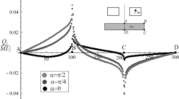
Figure 3 presents the distribution of normalized magnetic charges, Q _inor = Q _i∕ML ₁ ², along the boundary surface of two different magnetic materials. It’s been calculated for three different directions of the magnetization vector, for 𝛼 = 0, 𝛼 = 45° and 𝛼 = 90°, when configuration parameters are: a∕L ₁ = 1.0, b∕L ₁ = 1.0, c∕L ₁ = 5.0, L ₂∕L ₁ = 1.0, h∕L ₁ = 0.5, μ_r1 = 1, μ_r2 = 10, N _s = 300, N _v = 100 and N = 200.

Fig. 4.

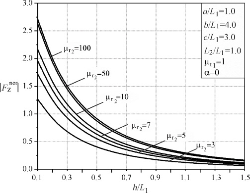
Axial magnetic force versus ratio h∕L ₁ for different cylinder permeability, μ_r2 in case of axial permanent magnet magnetization (𝛼 = 0).

After calculating the values of unknown magnetic sources, the magnetic scalar potential of soft magnetic cylinder can be determined from the expression $\begin{eqnarray}\displaystyle {\varphi}_{mc}={\displaystyle \frac{1}{2{\pi}^{2}}}\mathop{\sum }_{i=1}^{N_{\text{tot}}}Q_{i}{\displaystyle \frac{K\left({\displaystyle \frac{{\pi}}{2}},k_{i}\right)}{\sqrt{(r+r_{i})^{2}+(z-z_{i})^{2}}}}, & & \displaystyle\end{eqnarray}$ (14) along with magnetic field and magnetic flux density vector anywhere in the cylinder’s vicinity.

Final step is the calculation of the force between permanent magnet segments and toroidal magnetic sources. It is performed starting from the expression for the force between two circular loops loaded with different magnetic charges [17] and using the superposition of all contributions for permanent magnet’s magnetic charges and toroidal magnetic sources. This would give us the expression for the force between permanent magnet and the cylinder made of linear magnetic material placed in the environment of permeability μ₁ = μ₀: $\begin{eqnarray}\displaystyle \displaystyle F_{z}\text{} & =\text{} & \displaystyle {\displaystyle \frac{{\mu}_{0}}{2{\pi}^{2}}}\left(\mathop{\sum }_{n=1}^{N_{b}}\mathop{\sum }_{i=1}^{N_{\text{tot}}}\left(Q_{m1}Q_{i}P\left(r_{n},z_{1n},r_{i},z_{i}\right)+Q_{m2}Q_{i}P\left(r_{n},z_{2n},r_{i},z_{i}\right)\right)\right.\nonumber\\ \displaystyle \displaystyle \text{} & \text{} & \displaystyle \quad +∼\mathop{\sum }_{m=1}^{N_{c}}\mathop{\sum }_{i=1}^{N_{\text{tot}}}\left(Q_{m3}Q_{i}P\left(r_{3m},z_{m},r_{i},z_{i}\right)+Q_{m4}Q_{i}P\left(r_{4m},z_{m},r_{i},z_{i}\right)\right)\nonumber\\ \displaystyle \displaystyle \text{} & \text{} & \displaystyle \quad +∼\left.\mathop{\sum }_{p=1}^{N_{v1}}\mathop{\sum }_{k=1}^{N_{v2}}\mathop{\sum }_{i=1}^{N_{\text{tot}}}Q_{mv}Q_{i}P(r_{vk},z_{vp},r_{i},z_{i})\right),\end{eqnarray}$ (15) where $P(r_{0},z_{0},r_{i},z_{i})=\frac{(z_{0}-z_{i})E(r,r_{0},z,z_{0})}{((r_{0}-r_{i})^{2}+(z_{0}-z_{i})^{2})\sqrt{(r_{0}+r_{i})^{2}+(z_{0}-z_{i})^{2}}}$ , $\begin{eqnarray}\displaystyle E(r,r_{0},z,z_{0})=E\left({\displaystyle \frac{{\pi}}{2}},{\displaystyle \frac{4rr_{0}}{(r+r_{0})^{2}+(z-z_{0})^{2}}}\right). & & \displaystyle \nonumber\end{eqnarray}$

3. Numerical results

The obtained expression Eq. ((15)) is used for calculating the force between ring magnet and soft magnetic cylinder and determining the deviation of the force that is the result of magnetization vector misalignment. It is already confirmed in the previously published papers that deal with permanent magnet configuration [17], that it is not necessary to take a great number of permanent magnet segments in order to achieve high accuracy. For this system, the number of total surface segments is N _s = 300, while the total number of volume segments is limited to N _v = 100. The initial number of toroidal sources is limited to N = 200, in order to reduce the calculation time [18]. In this case the normalised magnetic force F _z ^nor = F _z∕μ₀ M ² L ₁ ² = −0.204579 is calculated for configuration parameters: μ_r1 = 1 , μ_r2 = 4, a∕L ₁ = 1.0, b∕L ₁ = 5.0, c∕L ₁ = 3.0, L ₂∕L ₁ = 1.0, h∕L ₁ = 1.0 and 𝛼 = 1°. The result of the used approach is compliant with the value obtained with finite element method (FEM). For that purpose FEMM 4.2 software was used, whereas F _z ^nor = −0. 204903, with relative error of 0.15%.

In the ideal case, when magnetization vector is aligned with the ring magnet axes of symmetry, 𝛼 = 0, normalized axial force versus normalized axial displacement of permanent magnet, h∕L ₁, is shown in the Fig. 4. It is presented for variable relative permeability of magnetic cylinder μ_r2 and for the system parameters: a∕L ₁ = 1.0, b∕L ₁ = 4.0, c∕L ₁ = 3.0, L ₂∕L ₁ = 1.0, μ_r2 = 1 and 𝛼 = 0.

As it often happens in practice, there is a certain misalignment of the magnetization vector, as it is considered in this paper, and the permanent magnet is not magnetized in the axial direction. Table 1 presents magnetic force intensity, for different magnetization vector inclination with respect to z-axis (different values of angle 𝛼), when the configuration parameters are: μ_r1 = 1, μ_r2 = 16, a∕L ₁ = 2.0, c∕L ₁ = 5.0, b∕L ₁ = 5.0, L ₂∕L ₁ = 1.0, h∕L ₁ = 0.5. Obtained results are compared with the force in the ideal case when permanent magnet is magnetized in the axial direction (𝛼 = 0). Relative error is actually relative deviation from the ideal case, and it will be also calculated as ${\delta}F_{z}=\frac{|F_{z({\alpha}=0)}-F_{z({\alpha}\neq 0)}|}{F_{z({\alpha}=0)}}$ . For these parameters, the misalignment of magnetization vector of 𝛼 = 1° leads to the relative deviation that is less than 1%. From the engineering point of view that deviation is completely acceptable.

Table 1
Magnetic force for different angles of magnetization vector misalignment

𝛼 [°] |F _z ^nor| δF _z [%]

0.0 1.11524 0

0.1 1.11619 0.085

0.2 1.11715 0.171

0.3 1.11811 0.257

0.4 1.11909 0.345

0.5 1.12007 0.433

0.6 1.12106 0.522

0.7 1.12206 0.611

0.8 1.12306 0.702

0.9 1.12408 0.792

1.0 1.12510 0.884

𝛼 [°]	\|F _z ^nor\|	δF _z [%]
0.0	1.11524	0
0.1	1.11619	0.085
0.2	1.11715	0.171
0.3	1.11811	0.257
0.4	1.11909	0.345
0.5	1.12007	0.433
0.6	1.12106	0.522
0.7	1.12206	0.611
0.8	1.12306	0.702
0.9	1.12408	0.792
1.0	1.12510	0.884

Fig. 5.

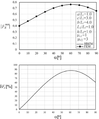
(a) Magnetic force dependency of misalignment angle 𝛼. (b) Relative deviation versus misalignment angle 𝛼.

On the other hand, when it comes to configuration parameters μ_r1 = 1, μ_r2 = 3, a∕L ₁ = 1.0, c∕L ₁ = 3.0, b∕L ₁ = 4.0, L ₂∕L ₁ = 1.0, h∕L ₁ = 0.5, the magnetization misalignment of 𝛼 = 1° leads to the greater deviation as it is shown in the Table 2. It is obvious that the influence of certain magnetization misalignment on the magnetic force, strongly depends on the configuration parameters. For this configuration, the deviation is significantly higher when the misalignment angle is 𝛼 > 1°. Linear change of the relative deviation could be seen in cases where the magnetization vector misalignment angle is less than 5 degrees (Tables 1 and 2).

Table 2

Magnetic force for different angles of magnetization vector misalignment

𝛼 [°]	\|F _z ^nor\|	δF _z [%]
0.0	0.398556	0
1	0.405318	1.69
2	0.412221	3.42
3	0.419255	5.19
4	0.426412	6.99
5	0.433683	8.81

In the Fig. 5a the normalized magnetic force intensity for higher inclination of the magnetization angle is shown using HBEM and FEM (FEMM 4.2 software). The configuration parameters are the same as the ones presented in the Table 2. The alignment of the results is evident. Results obtained are being compared with the ideal case (𝛼 = 0). Relative deviation vs. the misalignment angle 𝛼 is presented in the Fig. 5b, in order to illustrate the relative deviation of the magnetic force with the higher values of the angle 𝛼. Relative deviation is on the linear rise all the way up to 40°. After it peaks around 60° mark, it’s starting to fall, as the magnetization angle progresses towards 90°.

Fig. 6.

Axial magnetic force versus magnetization vector misalignment angle 𝛼.

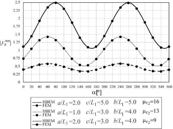
Magnetic force is presented in the Fig. 6 for all possible values of angle 𝛼. Common parameters in all three cases are L ₂∕L ₁ = 1.0 and h∕L ₁ = 0.5. The force is calculated using the HBEM and FEM in order to check the accuracy of the obtained results. It is visible that the influence of the misalignment angle dominates with thicker magnets. Maximal force is been reached when 𝛼 = 60° or 80° (depending on the case) and then it starts to fall. Also, along with the maximal force value obtained for the angle 𝛼 there is a corresponding, symmetrical, maximum for 𝛼 +180°.

Fig. 7.

Axial magnetic force versus ratio h∕L ₁ for different angles of magnetization vector misalignment.

Fig. 8.

Axial magnetic force versus cylinder permeability, μ_r2, for different angles of magnetization vector misalignment.

Fig. 9.

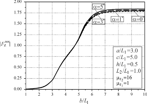
Axial magnetic force versus cylinder radius for different angles of magnetization vector misalignment.

Fig. 10.

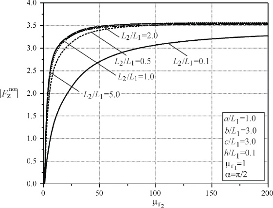
Axial magnetic force versus cylinder permeability, μ_r2, for different height ratio L ₂∕L ₁ in case of radial permanent magnet magnetization (𝛼 = π∕2).

In the case when 𝛼 = 90° and 𝛼 = 270°, force being determined equals the force of the magnet being magnetized in the radial direction. For 𝛼 = 180° force intensity equals the case when 𝛼 = 0, since that is the same magnet (with axial magnetization) but horizontally flipped.

As it was expected, values obtained for 𝛼 ranging between 0° and 180° are being repeated within the range of 𝛼 between 180° and 360°.

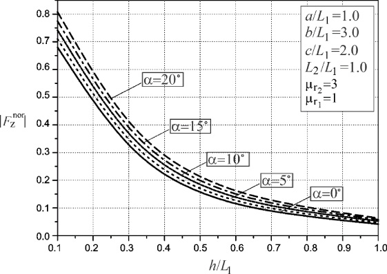
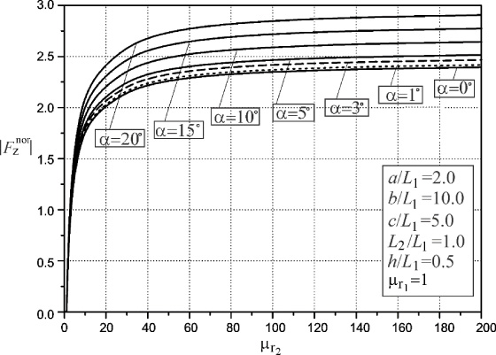
Figure 7 presents the axial force between permanent magnet and soft magnetic cylinder, versus normalized axial displacement of permanent magnet, h∕L ₁, for variable angles of magnetization vector misalignment. In this case the configuration parameters are: a∕L ₁ = 1.0, b∕L ₁ = 3.0, c∕L ₁ = 2.0, L ₂∕L ₁ = 1.0, μ_r1 = 1, μ_r2 = 3. Axial magnetic force versus cylinder permeability, μ_r2, for different values of angle 𝛼, is presented in the Fig. 8 for configuration parameters: a∕L ₁ = 2.0, b∕L ₁ = 10.0, c∕L ₁ = 5.0, L ₂∕L ₁ = 1.0, h∕L ₁ = 0.5, μ_r1 = 1.

From the Figs 7 and 8 it is obvious that there is a significant deviation of the results when the magnetization vector misalignment exists. For parameters used for calculation presented in the Fig. 8, the relative deviation goes from 1.38% in the case where misalignment angle is 𝛼 = 1°, 4.24% for 𝛼 = 2° to 32.9% for 𝛼 = 20°.

Figure 9 presents the magnetic field intensity versus magnetic cylinder radius in the case when misalignment angle 𝛼 varies from 0 to 5 degrees. In the case when the normalized cylinder radius is less or equal to the outer radius of the ring permanent magnet, the influence of the magnetization vector misalignment to the magnetic force can be neglected. When b∕L ₁ ≥ c∕L ₁ the relative deviation goes from the 0.57% for 𝛼 = 1° to 2.9% for 𝛼 = 5°.

By selecting the angle of magnetization vector inclination, the obtained expression for the force can be used for determining the force between radially magnetized ring permanent magnet and soft magnetic cylinder (𝛼 = π∕2). Figure 10 presents magnetic force, versus cylinder permeability, μ_r2 for different height ratio of permanent magnet and magnetic cylinder, L ₂∕L ₁ for the radially magnetized ring permanent magnet. Permanent magnet parameters are: a∕L ₁ = 1.0, b∕L ₁ = 3.0, c∕L ₁ = 3.0, h∕L ₁ = 0.1, μ_r1 = 1 and 𝛼 = π∕2.

4. Conclusion

The derivation of the magnetic force between soft magnetic cylinder and permanent ring magnet, in the case when the magnetization vector is not coincidental with axial axes, is presented in the paper. Majority of papers published by other researchers deal with interaction force between permanent magnet and infinite magnetic plain, while this paper illustrates the force calculation for configuration that contains object made of soft magnetic material with finite dimensions. Also, the calculation presented allows the inclusion of the permanent magnet vector misalignment in the design process of magnetic devices. The obtained results are compared with the ideal case values, for axially magnetized ring permanent magnet. It is very important to predict the influence that magnetization misalignment has on the magnetic field and magnetic force, since it is a common case that a geometrical axis of the permanent magnet is not precisely aligned with the magnetic axis of the domains in the permanent magnet. Since permanent magnets are primary component of great number of magnetic devices it is significant for device’s behaviour and quality. The derived expression can be also used for calculating the force between radial magnetized ring permanent magnet and soft magnetic cylinder and to determine the influence that displacement of radial magnetization have on the configuration behaviour. Results of proposed semi-analytical approach are in close agreement with FEMM 4.2 software results, but the advantage of this approach is faster and simpler force analyses in relation to the configuration parameters.

Footnotes

Acknowledgements

This work has been supported by the Ministry of Education, Science and Technological Development of the Republic of Serbia.

References

Yonnet

J.P.

, Passive magnetic bearings with permanent magnets, IEEE Transactions on magnetics 14 (1978), 803–805.

Yang

Zhou

Gong

and Li

, The numeric calculation for cylindrical magnet’s magnetic flux intensity, International Journal of Applied Electromagnetics and Mechanics 40(3) (2012), 227–235.

Yang

and Li

, Calculation of magnetic levitation force exerted on the cylindrical magnets immersed in ferrofluid, International Journal of Applied Electromagnetics and Mechanics 40(1) (2012), 37–49.

Bekinal

rao Anil

T.R.

and Jana

, Analysis of the magnetic field created by permanent magnet rings in permanent magnet bearings, International Journal of Applied Electromagnetics and Mechanics 46(1) (2014), 255–269.

Akoun

and Yonnet

J.P.

, 3D analytical calculation of the forces exerted between two cuboidal magnets, IEEE Transactions on Magnetics 20 (1984), 1962–1964.

Furlani

E.P.

Reznik

and Kroll

, A three-dimensional field solution for radially polarized cylinders, IEEE Transactions on Magnetics 31 (1995), 844–851.

Robertson

W.S.

Cazzolato

B.S.

and Zander

A.C.

, A simplified force equation for coaxial cylindrical magnets and thin coils, IEEE Transactions on Magnetics 47 (2011), 2045–2049.

Ravaud

Lemarquand

and Lemarquand

, Force and stiffness of passive magnetic bearings using permanent magnets. Part 1: Axial magnetization, IEEE Transactions on Magnetics 45 (2009), 2996–3002.

Vučković

A.N.

Ilić

S.S.

and Aleksić

S.R.

, Interaction magnetic force calculation of permanent magnets using magnetization charges and discretization technique, Electromagnetics 33 (2013), 421–436.

10.

Beleggia

Vokoun

and Graef

M.D.

, Forces between a permanent magnet and a soft magnetic plate, IEEE Magnetics Letters 3 (2012).

11.

Braneshi

Zavalani

and Pijetri

, The use of calculating function for the evaluation of axial force between two coaxial disk coils, in: Third International PhD Seminar on Computational Electromagnetics and Technical Application, Banja Luka, Bosnia and Hertzegovina, Proceedings of full papers (CDROM), 2006, pp. 21–30.

12.

Vučković

A.N.

Ilić

S.S.

and Aleksić

S.R.

, Interaction magnetic force calculation of ring permanent magnets using Ampere’s microscopic surface currents and discretization technique, Electromagnetics 32 (2012), 117–134.

13.

Rakotoarison

H.L.

Yonnet

J.-P.

and Delinchant

, Using Coulombian approach for modeling scalar potential and magnetic field of a permanent magnet with radial polarization, IEEE Transactions on Magnetics 43 (2007), 1261–1264.

14.

Perić

M.T.

Ilić

S.S.

Aleksić

S.R.

and Raičević

N.B.

, Characteristic parameters determination of different striplines configurations using HBEM, ACES Journal 28 (2013), 858–865.

15.

Raičević

N.B.

Aleksić

S.R.

and Ilić

S.S.

, A hybrid boundary element method for multilayer electrostatic and magnetostatic problems, Electromagnetics 30 (2010), 507–524.

16.

Perić

M.T.

Ilić

S.S.

Aleksić

S.R.

and Raičević

N.B.

, Application of Hybrid boundary element method to 2D microstrip lines analysis, International Journal of Applied Electromagnetics and Mechanics 42 (2013), 179–190.

17.

Vučković

A.N.

Raičević

N.B.

Ilić

S.S.

and Aleksić

S.R.

, Interaction magnetic force calculation of radial passive magnetic bearing using magnetization charges and discretization technique, International Journal of Applied Electromagnetics and Mechanics 43 (2013), 311–323.

18.

Vučković

A.N.

Raičević

N.B.

and Perić

M.T.

, Radially magnetized ring permanent magnet modelling in the vicinity of soft magnetic cylinder, Safety Engineering 8 (2018), 33–37.

19.

Meeker

, n.d. Software package FEMM 4.2. Available on-line at http://www.femm.info/wiki/ Download (accessed 2 March 2007).