Different regularization methods for an inverse magnetostatic problem

1. Introduction

Manufacturing processes for high field magnets usually include a number of quality checks to try characterizing possible discrepancies in the magnet layout with respect to nominal design, which, depending on the specific case, can produce relevant performance decrease in spite of their reduced amplitude. Examples of such high-performance magnets are the poloidal and toroidal coils in thermonuclear fusion reactors, the magnetic lenses in particle accelerators, the more common background field magnets in magnetic resonance imaging devices. Standard procedures rely on “optical” surveys, but deformations coming after insertion in the case and final assembly are not detectable with such approaches; external magnetic measurements have been proposed to estimate the possible deformations of conductors inside the magnet. In the following, the attention will be limited to large (superconducting) high field magnets, as for example those used in devices for Thermonuclear Fusion [1,2], but many of the exposed results can be easily extended to other type of problems [3–5]. During the magnetic testing, these coils are energized at room temperature, with a reduced current supply. A schematic view of the measurement layout, with reference to a circular coil with a Winding Pack (WP) of 25 conductors, arranged in 5 layers, is sketched in Fig. 1.

OPEN IN VIEWER

Fig. 1.

Sketch of the measurement layout for a circular coil.

Taking into account: (i) the limitations on the frequency, that must be very low to avoid inducing eddy currents in the metallic case and support structures, (ii) the expected amplitude of the field, in the order of few mT in the considered case, and (iii) the need of measuring the field with high spatial resolution to catch the small local field map variation induced by deformations, in this study the underlying measurement system is assumed to be based on a set of Hall probes, fixed to a plastic holder encircling the magnet. This “system” is used to measure simultaneously the tangential component of flux density in N _p points, repeating the process in N _s sections along the coil. The difference between the nominal and the actual field map (the magnet “field error”) is expected to be very small compared to the nominal field, since manufacturing and assembly tolerances are typically very tight in the case of high accuracy manufacturing processes. Consequently, the measurement procedure is quite demanding, as it must appreciate small field variations in presence of noise, background field and other nuisances. The estimation process must then be carefully designed, considering both the measurement system characteristics and the data processing, since the reconstruction implies the treatment of the problem ill-posedness.

The attention is here focused on the possible methods to regularize the described estimation problem. A brief description of the numerical methods used to simulate the measurement process is first given, with reference to a circular coil for the sake of simplicity. The considered regularization methods are then briefly recalled. A comparison of the different methods is then illustrated, and finally some discussion of drawbacks and advantages is reported.

The magnets characterization problem involves the computation of the flux density generated by a magnet affected by known deformation (described by a trial deformation parameters array p ) in a set of measurement points x _mi , i = 1 , … , N p ∗ N s . In the hypothesis of magnets operating in DC, in free space, the flux density can be computed using the Biot-Savart law: (1) where x _s is the source point, r _ms is the vector joining x _s to x _mi , J is the current density and 𝛺 _s is the volume where current is flowing. In order to compute (1), the current density J is discretized in N _WP filamentary coils, as many as the conductors in the WP. Due to the presence of symmetry-breaking deformations, it is not possible to use analytical expressions for circular filamentary coils, and each deformed conductor is described by a polynomial spline (commonly known as a NURBS), defined using a limited number of knots, whose positions in space are defined, starting from the nominal design coil centerline, by p . Each conductor is then discretized into N _seg current segments by N _bp = N _seg + 1 break points 𝜉 _k (typically, N _bp is much larger than the number of NURBS knots).

OPEN IN VIEWER

Fig. 2.

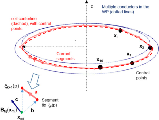
Schematic view of coil discretization into current segments.

The total field in each measurement point x _mi is finally computed by summing up all the contributions of single segments, adopting the analytical expression available for this elementary source [6]: (2) (3) where a, b, c, 𝜉 _k have been defined in Fig. 2 (the upper index in 𝜉 referring to the conductor index in the WP), the dependence of 𝜉’s on p has been highlighted for the sake of understanding, I _cnd is the segment current (equal for all segments and all conductors, since all of them are assumed to be series connected), and b _stick is the field of a segment fed by a unit current. Note that when the geometry is known, the double summation can be pre-computed for each measurement point, providing an array of “unit-current” flux densities on the probes. m _ u n i t ( p _ ; x _ m ) = ∑ j = 1 N W P ⁡ ∑ k = 1 N b p − 1 ⁡ t ^ k j ⋅ b stick ( ξ k j ( p _ ) , ξ k + 1 j ( p _ ) ; x _ m ) , t ^ k j being the tangent versor of the (j, k)-th current segment, and x _m is the array containing the measurement points coordinates. Actual measurements will then be given by: (4) where ϵ _mdl is the error introduced by the modelization of the actual coil through N _WP ^∗ N _seg current elements. In the remaining of this section, the dependence of m on p and x _m will be omitted for the sake of readability.

As anticipated, in the additional hypothesis of very small variation δ p of “shape parameters” with respect to the unperturbed value p ₀, the variation of m can be approximated by a first order Taylor expansion with respect to δ p : (5) where m ₀ = m ( p ₀, x _m ), ϵ _lin (|δ p |²) is the “linearization” error, and the element s _{i, n} of the sensitivity matrix S , corresponding to the variation of the i-th measurement (at point x _i ) with respect to the n-th deformation parameter p _n , is defined as: (6) The process of estimating the deformation parameters p reduces then to: (7) where ϵ = ϵ _mdl + ϵ _lin + ϵ _noise , and m ∼ _ is the array of actual probes measurement on the built magnet. Note the actual measurements corresponding to the nominal, design magnet are not available “by definition”, since any built magnet will unavoidably be affected by tolerances, and this obliges to adopt simulated measurements m ₀ as a reference, providing a relevant additional component in the model error.

Due to the ill conditioned nature of S , suitable countermeasures are required to keep the effect of nuisances ϵ as limited as possible, e.g. by adopting some kind of regularization in the inverse problem resolution. Although the actual problem is non-linear with respect to deformation parameters, as anticipated, a linearized approach has been adopted in this study, whose applicability will be assessed in the next section with reference to the expected deformation ranges (See Fig. 3); consequently, in the remaining of the paper mainly regularization schemes for linear problems have been considered.

Since the seminal proposal of Tikhonov [7], many regularization algorithms have been proposed to counteract the ill conditioning of linear inverse problems. In the authors’ view, a general yet rough subdivision should include direct algorithm, iterative algorithm and machine-learning algorithms [8–10], although some of the latter (e.g. Artificial Neural Networks, ANN) are able to deal also with non-linear problems. A different approach considers simultaneously the solution and the uncertainties, both on the solution itself and on uncontrolled parameters (see, e.g., [11]). The aim of this approach is to estimate the solution uncertainty rather than affecting the structure of the inverse operator as defined in (7), and will not be further considered here.

In this comparative study, we have considered:

–

Direct algorithm: Tikhonov Regularization (TR) [7], Truncated Singular Value Decomposition (TSVD) [12] and Damped Singular Value Decomposition (DSVD) [13], Constrained Least Squares (CLSQ) [14], and Discrepancy Principle (DP) [15];

–

Iterative Algorithms: Conjugate Gradient (CG) [16], 𝜈-method (𝜈M) [17], Algebraic Reconstruction Technique (ART) [18];

–

Machine-Learning methods: Bayesian ANN (B-ANN) [10].

The list is in no way complete, nor the results can be generalized in our opinion. In order to better frame the following results and comparisons, we provide in this section a short description of each method.

OPEN IN VIEWER

Fig. 3.

Deviation of the measured field with respect to the nominal value due to different deformation parameters on probes at section #4, lying in the allowed region. All other probes behave similarly.

OPEN IN VIEWER

Fig. 4.

Left: Structure of the S matrix considering all measurements (blue) and neglecting those below the uncertainty level for deformations parameters at the highest allowed value. Right: distribution of singular values for both “red” and “blue” matrices.

–

TR: this is probably the best-known regularization method, and bases on the minimization of a linear combination of the discrepancy and of the solution vector in a suited norm, the usual choice being L ₂ norm. The resulting formulation can be stated as: p _ T R = min p _ ⁡ ( ‖ S _ _ p _ − m ∼ _ ‖ 2 + λ ‖ p _ ‖ 2 ) . The key element for the success of the method is the choice of the regularization parameter 𝜆. A too large value can in fact provide a very “smooth” solution, not minimizing the measurements discrepancy ‖ S _ _ p _ − m ∼ _ ‖ 2 . The most common approach to the choice of 𝜆 is through the 𝜆-curve [8], but Generalized Cross Validation (GCV) [19] provides a relevant alternative. GCV excludes some of the measurements during the estimation process, and then selects the value of 𝜆 providing the value of p best fitting the excluded measurements. Both 𝜆-curve and GCV do not rely on information about measurement error, but rather try to self-adapt using available measurements only.

–

TSVD: this method is based on the SVD of the matrix, S =𝛴 _i=1…N   u _i σ _I v _i ^T , where u _i and v _i are the (column) arrays of left and right singular vectors, respectively, and the singular values σ _i , i =1…N, are ordered from highest to lowest. The conditioning number of S is given by σ₁∕σ _N . By standard matrix algebra, it is possible to show that the least squares solution to the estimation problem (7) is given by: p _ S V D = ∑ i = 1 , N ⁡ ( u _ i ⋅ m ∼ _ ) / σ i v _ i . In ill-conditioned problems, the Fourier coefficients u _ i ⋅ m ∼ _ corresponding to highest order singular values do not decay as fast as the corresponding singular values. This condition is a discrete equivalent of the Picard condition for continuous problems [9], and it’s profitable to verify how higher order spectral components in the data array m ∼ _ are enhanced by plotting the weighted Fourier coefficients ( u _ i ⋅ m ∼ _ ) σ i (see Fig. 4). The TSVD approach consists in truncating the summation to the index k ^∗ corresponding to the numerical rank of S , that is the index of the last singular value higher that the error ϵ: p _ T S V D = ∑ i = 1 , k ∗ ⁡ ( u _ i ⋅ m ∼ _ ) / σ i v _ i . In this case the truncation index k ^∗ plays the role of a regularization parameter.

–

DSVD: in the case of Damped-SVD, instead of neglecting the contribution of higher order singular vectors, the corresponding Fourier coefficients are weighted by a damping term: p _ D S V D = ∑ i = 1 , N ⁡ ζ i ( u _ i ⋅ m ∼ _ ) v _ i where ζ _i = σ _i ∕(σ _i + 𝜆).

–

CLSQ: as noted above, the resolution of (6) using the plain SVD (equivalent to least squares minimization of discrepancy for over-determined problems) leads to inaccurate results, at least for ill conditioned problems such as the one at hand. If a reasonable bound δ can be determined for some norm of the parameters array p (e.g., the L ₂ norm), it is possible use a constrained minimization of the L ₂ norm of discrepancy, leading to the CLSQ regularization approach:

–

DP: the CLSQ approach relies on some estimate for the p norm upper limit, which is not easy to get. Basing on the more usual availability of an upper limit to the norm of the discrepancy between field map reconstruction and actual measurements based on the overall measurement uncertainty, the DP method amounts to minimizing some norm of p (e.g. L ₂) with the constraint that the L ₂ norm of the discrepancy must be less than the limit imposed by measurement accuracy:

–

CG: the conjugate gradient algorithm, applied to the unregularized equation, transformed into normal form S _ _ T S _ _ p _ = S _ _ T m ∼ _ to ease CG application, can be described by the following steps: The algorithm is initialized by r _ 0 = S _ _ T m ∼ _ . It is observed that the components of the k-th iteration solution array, p _k , corresponding to the largest singular values tend to converge faster. This can be demonstrated [9], but it is out of the scope of the present discussion. Consequently, the CG algorithm can be seen as a regularizing one, with the iteration index k playing the role of a regularization parameter. Note that the solution p _CG ≡ p _k∗ is quite sensitive to the choice of the stopping iteration number k ^∗.

–

𝜈M: the 𝜈-method aims explicitly to slowing the convergence of CG algorithm, in order to make the solution p _𝜈M less sensitive to the choice of k ^∗. This is achieved by using an update of 𝛼 _k and 𝛽 _k parameters based only on the iteration number k and on a parameter 𝜈 ∈ ]0,1[:

–

ART (Kaczmarz method): the solution p _k is corrected stepwise, according to one row of S : p _ k − 1 + m ∼ k − ( s _ T ) k p _ k − 1 ‖ s _ k ‖ 2 → p _ k k = 1 , … N An iteration is completed when all the rows in S have been considered. ART does not involve matrix multiplication, and it converges slower than CG.

–

B-ANN: although in the authors’ opinion deep-learning approaches appear quite promising for estimation tasks, just a standard ANN with sigmoidal activation functions and a single hidden layer has been considered in this study. The training paradigm is a variation of the classical Levenberg-Marquardt called “Bayesian regularization” [10].

4. Sensitivity matrix analysis

For the sake of exposition, in the following we will refer to a circular coil, with a radius R _coil = 8 m, a WP of 5 layers of 5 conductors each (N _WP = 25), fed by a DC current of 1 kA. We will consider two classes of deformations, local and global. Global deformations are radius increase/decrease along x and y axis (an ellipticization, defined by 𝛾 _x and 𝛾 _y parameters, with a bound of ±30 mm), tilt around y axis (θ _y parameter, with a bound of ±0.15°) and rotation around z axis (θ _z , required to generalize the ellipticizations and tilts). In order to define local parameters, let us introduce the concept of “control point”. The coil shape can be defined using a “WP centerline”, describing the overall geometry of the coil (a circle in this study), and the positions of the conductors inside the WP at any cross section along the centerline. Any non-circular shape (including the deformations of a circular shape) requires some general curve, e.g. a spline, defined in terms of a collection of points in space, called Control Points (CP). In our study, we considered 10 CP, evenly distributed around the coil. Local parameters can now be defined as radial and vertical displacements of CP (δR _k and δz _k , k = 1,2…10, with a bound of ±20 mm), plus a rotation of the WP around the centerline at the CP section (θ _WPk , with a bound of ±5°). The total number of deformation parameters is then N _DOF = 34. The measurement data are provided by 12 tangential probes, evenly distributed in 7 circumferences with a radius R _meas = 0.3 m. The centers of circumference are located at 7 points on centerline, distributed only on a 270° angle, to simulate an “exclusion region” on the coil, located near the joint of the inner windings to the current feeder. Probes are affected by a normally distributed uncertainty, with a standard deviation of 0.2% of the full-scale value (20 mT). We have then N _meas = 84 measurements to identify the 34 Degrees of Freedom (DOF). As anticipated above, the problem at hand considers the relationship between magnetic field around a coil and the geometry of the latter. As a general rule, this dependence is nonlinear, but when considering just small deformations, the effect on the field map deviations from its nominal configuration can be linearized, as stated in ((5)). Note that the linear dependence has to describe this relationship only within an accuracy not better than the measurement uncertainty to be valid.

Since the probes measure the total field of the magnet (slightly less than 20 mT in the described configuration), but the impact of deformations is much smaller (tens or hundreds of μT), the impact of the uncertainty strongly limits the sensitivity of the measurement system. As a consequence, the linear model is applicable within the tolerance limits introduced above. A second consequence is that any value of deformation parameters less than 5 mm (or 1/4 of the bound) is considered unreliable, since the measurement variation generated by so small deformations is below the uncertainty level.

In Fig. 3 a few examples of measurements dependence from some of the DOFs at one measurement section are reported, showing that a linear model is suited for this analysis. Figure 3c shows in addition that the impact of local deformations is mostly limited to measurement sections neighboring the control section where the CP is defined.

OPEN IN VIEWER

Fig. 5.

Picard condition for the full matrix (a), excluding non-detectable DOFs (b), also DOFS in exclusion area (c) and for detectable local DOFs only (d).

The sensitivity matrix S has then 84 rows and 34 columns. Its structure is reported in Fig. 4 (blue and red dots), and has full rank, but a conditioning number of 1.0 × 10⁷. On the other hand, if we consider the sensitivity of probes, and neglect any entry in S less that 4 μT, the structure reduces to the red dots in Fig. 4. In this case, the conditioning number is not limited, and the rank is 19, clearly showing the ill-posed natured of the underlying problem. Singular values distribution is reported in Fig. 4b for both the blue and the red matrix.

The filtered matrix still shows a few columns of zeros, indicating that some DOFs (namely, those related to rotations and those describing local deformations in the excluded area) are not detectable using the proposed measurements. If columns corresponding to non-observable DOFs are removed, the corresponding matrix still shows a large conditioning number, indicating the presence of multiple solutions. This is due to the possibility of obtaining global ellipticization using suited combinations of local radial displacements. If we could exclude also global DOFs, the corresponding matrix would have a conditioning number equal to 10.4 and full rank. On the other way, in the following we will keep global DOFs, as the main focus in this study is the possibility to keep all detectable DOFs, comparing different regularization schemes. The behavior of Fourier coefficients with respect to corresponding singular values (discrete Picard condition [9]) is reported in Fig. 5, for the different matrices considered insofar, and for measurements corresponding to a random (yet typical) set of deformations. Note that when considering only DOFs associated sections in the allowed area (instrumented sections, meaning that measurements are available on the corresponding section), number of singular values σ _i larger than the corresponding Fourier coefficients |u _i m _i | reduces markedly.

All the considered different regularization schemes do possess some parameter that must be optimally chosen. By using GCV approach for direct method, the results in Table 1 are obtained, for a representative test case. Different cases do provide quite similar results. As concerning iterative methods, the selection of the optimal iteration index k ^∗ has been done by graphical inspection of surface plots of DOFs vs. the iteration number (see an example for ART in Fig. 6). Results are also reported in Table 1.

OPEN IN VIEWER

Fig. 6.

Different DOFs estimates from ART for increasing number of iterations. The reference values of DOFs are the same as for Table 1.

From a comparative analysis of the results, it is possible to note that the unregularized SVD is not able to recover deformations, while the classical Tikhonov approach achieves a reasonable estimation of deformed geometry. Also iterative approaches manage to deal with uncertainties, but with larger final errors. The above cited possibility of obtaining “elliptical” magnets either using global 𝛾 _{x, y} parameters or by combinations of local δR _k ones reflects in a significant error bar on both 𝛾 _x and 𝛾 _y .

The results considered up to now are obtained from numerically generated measurements, using the MISTIC code, based on (2)–(3) [6]. Although MISTIC considers the nonlinear relationship between geometrical DOFs and magnetic field, an inverse crime issue is still present. Consequently, we used a 3D FEM model to generate measurements with a different numerical approach. Allowed deformations in the FEM model are 𝛾 _x , 𝛾 _y and θ _y . In the proposed approach, tilts have been removed from allowed DOFs, but a tilted magnet can still be represented using local deformations δz . Figure 7 shows the deformed coils (enhanced for the sake of readability), while Fig. 8 reports a comparison between FEM data for a deformed configuration and MISTIC data for the reference one. Note that the data used for the estimation are the difference between FEM (deformed) and MISTIC (nominal) measurements. If this difference would have been less than accuracy, than any effect would have been not observable. On the other hand, using a different model than the one used to compute S introduces a much higher model error ϵ _mdl . Results of the estimation process are reported in Table 2 for the regularization methods providing best performance with self-generated data. It is possible to recognize that both methods were able to detect the “radial” nature of the deformation in the first case, ignoring DOFs for z displacement, and the “vertical” nature in the second case, ignoring DOFs for radial displacements, but the exact nature of the deformations were not recognized.

OPEN IN VIEWER

Fig. 7.

Sketch of the deformed (blue) and nominal (grey) coils used for FEM simulations. Left: ellipticization, Right: tilt. Deformations are amplified for the sake of readability. Measurement circumferences are also reported (thin lines across grey coil).

OPEN IN VIEWER

Fig. 8.

Comparison of numerical measurement generated by FEM model for deformed coils and by MISTIC for nominal coil. Left: Ellipticization, Right: Tilt. For both cases, the difference is above the uncertainty threshold, but the model error ϵ _mdl is much higher.

In this paper we have considered the regularization of an inverse problem typically encountered in the tolerance assessment of high field magnets at the end of production process from external magnetic measurements. The motivation of this work are in the feasibility analysis for a magnetic survey system to monitor tolerances in the manufacturing of toroidal field coils for the ITER tokamak [20]. The main characteristics of this class of estimation procedure is the relatively small amplitude of the “relevant” signal, which is the difference of field map with respect to the design one, due to very small deviations of the built magnet from the reference design. As a matter of fact, the useful signal is hidden in the much stronger main field, obliging the probes to adopt a full scale suited to measure the full field, and driving as a consequence the absolute value of uncertainty to values comparable to useful signal also in the case of very sensitive probes. The second issue is the unavailability of a “reference” map, generated by a “design” magnet, since the manufacturing process, whose tolerances we are trying to assess, is already pushed at its best in the case of high-performance magnets. A further consideration must be done on the choice of deformation parameters. In this study, we have adopted a realistic description of the magnet geometry, as typical for magnets manufacturers, which lead to a non-unique definition of some deformed configurations. The adoption of suited regularization schemes allows us to deal with such redundancy, at least in the case of self-generated data. In the case of “measurements” simulated using a different approach, the regularized estimation procedure was able to detect the “nature” of the deformations (vertical or radial), but not to isolate global deformation parameter from local ones. The comparison of results achieved using the same model for deformed and nominal configurations and those achieved when the models were different shows that the availability of a model of the nominal magnet able to describe accurately the actual device (and not its numerical model) is a key issue for the success of the estimation.

Notably, the adoption of machine-learning based approach (an artificial neural network with sigmoidal activation functions, trained with a probabilistic scheme) lead to poor results, in spite of the relevant computational effort required to train the network. In our opinion this indicates that the regression model for this class of approaches must be carefully chosen, together with the examples in the data set used to train the network.