Application of orientation distribution functions’ theory in the case of grain-oriented steels cut through classical and non-conventional technologies

Abstract

Grain-oriented silicon iron alloys present an important magnetocrystalline anisotropy, which has a strong influence on the normal magnetization curve and the energy losses. The theory of Orientation Distribution Functions (ODF), applied in the case of materials presenting crystalline symmetry of body centered cubic structure and orthorhombic strip symmetry, is taken into consideration. The magnetocrystalline anisotropy is analyzed on JFE Steel Corp. commercial grade M-0H grain-oriented electrical steel, cut at different angles with respect to the rolling direction, ranging from 0° to 90° in equal steps of 15°. The accuracy of the ODF method is analyzed by taking into account firstly three sets of experimental data, obtained for 0°, 45°, and 90°, then four sets, in the case of 0°, 30°, 60°, and 90° cut samples, and in the last case for all seven directions. The magnetic properties are predicted for any arbitrary direction and a relative error is analyzed, in each case, between the experimental and the numerical data. Finally, a proper number of experimental measurements was chosen, by considering a compromise between the magnitude of the error and the amount of experimental data. The samples were cut through mechanical punching, laser and travelling wire electro-erosion technologies. The normal magnetization curves and the energy losses were measured utilizing an industrial single strip tester (SST), at the frequency of 50 Hz. The model presented in the paper is a useful tool in the electric transformer cores’ design since every magnetic property could be predicted with an increased accuracy in the case of each angle.

Keywords

Grain-oriented alloys energy losses orientation distribution functions magnetocrystalline anisotropy normal magnetization curve punching laser cutting electro-erosion

1. Introduction

Grain-oriented electrical steel alloys (FeSi GO) have superior magnetic properties in the rolling direction (RD) [001], due to their metallurgically induced Goss texture. The increased number of grains that have their easy magnetization axis of [001], oriented parallel to the RD, determines high values of the magnetic permeability and low energy losses. In practical applications, the grain-oriented steels can be excited along different directions with respect to the lamination axis. The domain structure of the material is strongly influenced by the applied magnetic field; it depends on the crystal shape and magnetic domain arrangement within the magnetic core.

The most important crystallographic directions, for a FeSi single crystal with (110) oriented surface, are [001] and [11̄0]. These axes have a correspondent in a real FeSi lamination to the rolling (RD) and transversal (TD) directions, respectively, but with a few degrees of uncertainty. Classical approaches take into consideration an average interpolation of the magnetization curves, experimentally determined along RD and TD, to predict the J (H) dependence at different angles, with respect to the RD. These empirical computations have important limitations in the magneto-crystalline anisotropy analysis of the grain-oriented FeSi strips [1–4].

The magneto-crystalline anisotropy is due to the spin-orbit interactions [5–7]. This fact is directly linked to the molecular structure of the crystal, and it is present, in the case of FeSi GO, in which the body centered cubic structure of the pure iron is improved, to introduce a hard magnetization axis along the diagonal of the cube. Anisotropy of magnetic properties is intensively exploited nowadays, in order to manufacture electrical devices with high-energy efficiency [8,9]. The magnetic cores of these electrical devices have parts with different orientations with respect to the RD. Consequently, electrical engineering designers would require knowing where magnetic reluctivity is minimal. A real disadvantage is that the anisotropy phenomenon of the grain-oriented silicon iron alloys is usually neglected, and, as a result, catalogs provide only measured data for the RD and for the direction perpendicular to the rolling direction (TD) [111], as specified by international standards (EN 10107, JIS C 2553 and ASTM A876) [10].

The grain-oriented electrical steel sheets are usually cut through mechanical punching technology, which leads to induced mechanical stresses, near the cut edge thus influencing the crystallographic texture and the magnetic properties of the device cores. Due to punching, burrs appear at the edge of the strips, which deteriorate the interlaminar electrical insulation and generate small airgaps during the stacking core process. The laser technology determines a burr free cut edge, which does not present mechanical deformations, the magnetostrictive effect being also absent in this area. The main disadvantage of the laser cutting is the induced thermal effect in the cutting zone that could have a negative impact on the grain orientations and, as an unwanted result, oxide deposits may appear at the cut edge [11]. When the cut is made through electro-erosion, it results a high-quality cut edge on the upper side and burs on the lower side. The cutting speed could be adjusted, although the process is slow. In the case of travelling wire electrical discharge machining (TW EDM), a vertical moving electrode is involved, which is tensioned using a mechanical tensioning device, making possible in this way a cutting error reduction. Steel is eroded, due to the wire movements, and, because there is no contact between the sample and the travelling wire (TW), the induced mechanical stresses are minimized [12].

The quantitative mathematical analysis of the crystallographic texture has been treated in literature [13–15] and it can be considered that crystal orientation is a very important parameter [13]. Texture of the material is linked to the orientation distribution function (ODF) of the crystallites, which contains only angular variables that describe the crystal axes’ orientation with respect to a reference direction in the sample (i.e. the RD). The ODF does not take into consideration the spatial position of the crystals, their geometrical properties and their neighborship relations [13,14]. According to the classical approach, the crystals are assumed to be ideal, excepting their finite size, although in a real material the crystallites contain lattice defects as interstitial atoms, impurities and dislocations. In this case, if the crystal imperfections are not linked with the crystal orientation, the classical concept could be applied, by considering them as ideal ones, but with modified properties. The microscopic anisotropies of the crystals are usually averaged out, but the result is different from zero, so a macroscopic anisotropy is present in the material. FeSi GO steels could be considered as a micro inhomogeneous media from the point of view of anisotropy and this phenomenon could be therefore analyzed by taking into consideration the texture.

2. Anisotropy analysis with ODF theory

The grain-oriented silicon iron strips are characterized through orthorhombic symmetry of body centered cubic crystals and the Goss texture (110)[001] samples could be analyzed with the ODFs theory. The magnetic properties versus angle θ, measured with respect to the RD, can be computed as a series of trigonometric functions [16–18].

In [19,20] it is put in evidence that any magnetic properties A can be described with a series of ODF parameters as: $\begin{eqnarray}\displaystyle A=A_{0}+\mathop{\sum }_{i=1}^{n-1}A_{i}\cos (2i{\theta}), & & \displaystyle\end{eqnarray}$ (1) where n can be associated with the number of characterized samples. The coefficients A ₀ and A _i are determined from experimental data, which are the normal magnetization curves J (H) or energy loss variations W (J), measured for the samples cut between 0° and 90° with a given step.

For an imposed value of the magnetic field strength H ₀ a linear system of equation can be generated as: $\begin{eqnarray}\displaystyle \left[\begin{array}{@{}cccc@{}}1 & \cos (2{\theta}_{1}) & \cdots ∼ & \cos [2(n-1){\theta}_{1}]\\[5.0pt] 1 & \cos \left(2{\theta}_{2}\right) & \cdots ∼ & \cos [2(n-1){\theta}_{2}]\\[5.0pt] \vdots & \vdots & \cdots ∼ & \vdots \\[5.0pt] 1 & \cos (2{\theta}_{n-1}) & \cdots ∼ & \cos [2(n-1){\theta}_{n-1}]\end{array}\right]\left[\begin{array}{@{}c@{}}A_{0}(H_{0})\\[5.0pt] A_{1}(H_{0})\\[5.0pt] \vdots \\[5.0pt] A_{n-1}(H_{0})\end{array}\right]=\left[\begin{array}{@{}c@{}}A(H_{0},{\theta}_{1})\\[5.0pt] A(H_{0},{\theta}_{2})\\[5.0pt] \vdots \\[5.0pt] A(H_{0},{\theta}_{n-1})\end{array}\right], & & \displaystyle\end{eqnarray}$ (2) from which the values of the vector [A _i(H ₀)] can be computed. This algorithm may be repeated in the case of different values of the magnetic field. Another method for the A _i parameter computation is described in [21] and is based on fast Fourier transformation (FFT), which leads to a high accuracy of the model, using a reduced number of experimental data.

3. Materials and methods

In this paper, in order to apply the ODF theory in the case of grain-oriented alloys, M-0H grade steel samples, cut at angles θ ranging from 0° to 90°, with a 15° increment, were prepared and the value of decomposition order n was established at 7. The industrial grade M-0H laminations were cut as strips of 300 mm × 30 mm, with the thickness of 0.27 mm, through mechanical punching, laser and electro-erosion cutting technologies. The following cutting equipment was used: Trumpf Trumatic Punch 500 (mechanical), Trumpf CO2 Laser 3030 Classic (laser) and Sodick Wire EDM VL600Q (electro-erosion), respectively. The samples were characterized with a Brockhaus Messtechnik unidirectional Single Strip Tester, that has a digital control of the sinusoidal magnetic flux density waveform according to the standard IEC 60404-3. The measuring frequency was set at 50 Hz for 33 different imposed values of magnetic field strength starting with 5 A/m up to 10 kA/m. The form factor of the secondary voltage was kept for all measurements within the interval 1.1102 ± 0.4%.

To compute the A ₀ and A _i coefficient of the cosine series (Eq. (1)) a numerical program was developed and implemented in MATLAB.

4. Results and discussions

4.1. Normal magnetization curve

The normal magnetization curves were determined as the geometric place of the symmetrical hysteresis cycle maximum tip points, which consist of magnetic polarization and applied field peak values extended from the demagnetized state to saturation.

Figure 1 shows the computed and the experimental data, measured in the case of mechanically cut samples. The experimental data used in the analytical model are based on three, four and seven predefined angles θ. It can be noticed that, through Eq. ((2)), there is a very good accuracy in predicting the normal magnetization curve in the case of the angles for which the input data J(H) were considered. With the use of an increased number of J(H) curves, the error between experimental and computed values is decreased.

Fig. 1.

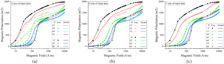
Normal magnetization curves determined in the case of samples cut through punch technology (full line represents data computed corresponding to the model introduced by Eq. (2), using as input: (a) three sets, (b) four sets and (c) seven sets of experimental measurements).

It can be observed from Fig. 1(a) and (b) that, if three or four coefficients, experimentally determined from data obtained for θ of 0°, 45°, 90° and 0°, 30°, 60°, 90°, are used, the low magnetic field strength region, below 100 A/m, cannot be correctly investigated and modelled. The explanation consists of the fact that in the cosine series from Eq. (1) may appear some mathematical “oscillations” that are directly linked to false physical properties such as a negative magnetic permeability [19,20,22–26].

Fig. 2.

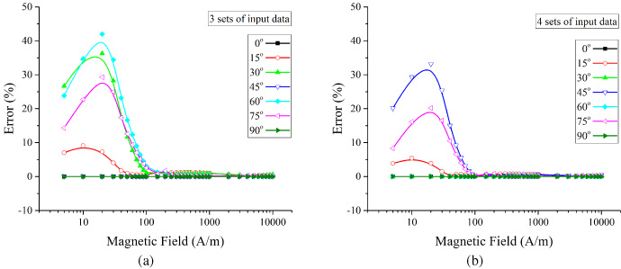
Relative error in the case of samples cut through mechanical cutting technology versus magnetic field strength (error = ((J _exp – J _comp)/J _exp)∗100) for (a) three sets and (b) four sets of experimental measurements.

In the case of seven experimental measurement data sets, the differences between experimental and computed dependencies are very low (Fig. 1(c)) and the model predicts in an adequate manner the normal magnetization curve for all the θ values. It was calculated the relative error between the experimental J _exp and predicted J _comp magnetic polarization data (Fig. 2) for the reduced number of input parameter. In both cases of mechanical cutting analysis, the error is below 45% (3 sets of input data) and 35% (4 sets of input data) for values of magnetic field strength lower than 200 A/m.

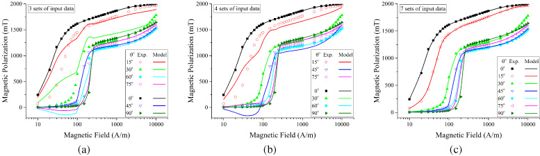
Figure 3 shows the computed and the experimental data, determined in the case of laser cut samples. Due to the induced thermal stresses at the edge of the strips, the experimental J(H) dependencies indicate a harder magnetization process than in the case of mechanically cut samples when the applied magnetic field strengths have a higher value.

Fig. 3.

Normal magnetization curves determined in the case of samples cut through laser technology (full line represents data computed corresponding to the model introduced by Eq. (2), using as input: (a) three sets, (b) four sets and (c) seven sets of experimental measurements).

For the laser cut samples, when using as input data three and four sets of experimental measurements, some instabilities of the model are present for magnetic field values comprised between 100 A/m and 1000 A/m, in the case of samples cut at 15° and 30° (Fig. 3(a)) and for the 45° strip (Fig. 3(b)). These model instabilities could be due to the induced thermal stresses, during the laser cutting procedure, and to the demagnetization effects generated by the existence within the sample of some non-magnetic regions. Such non-magnetic regions are due to the increased temperature above the melting point and an uncontrollable consequent cooling process [27–32]. Nevertheless, the overall relative error for this type of cutting technology is lower than in the cases of punching or electro-erosion methods, with a maximum value of 25%.

Fig. 4.

Normal magnetization curves determined in the case of samples cut through electro-erosion technology (full line represents data computed corresponding to the model introduced by Eq. (2), using as input: (a) three sets, (b) four sets and (c) seven sets of experimental measurements).

The electro-erosion technology has an impact on the magnetic domain structure, although this method is based on an eroding phenomenon, which has no visible plastic deformation and it determines the existence of very small burrs near the cut edge [27,28].

The TW EDM procedure generates tensile residual stresses, which have an impact on the normal magnetization curve. It can be observed from Fig. 4(a) and Fig. 4(b) that the model presents some instabilities in the low magnetic field strength region. Moreover, in the case of three parameter-based computation, differences between experimental measurements and predicted values are present for the 15° and 30° and for the four parameter-based model this behavior is present for the 45°, but the relative errors for these cases are higher (around 60%) than those obtained for punching and laser cut procedures. By comparing the EDM cutting procedure with the laser technology, it can be noted that, in the case of EDM, in the magnetization process, the strip needs lower values of the magnetic field strength, which is probably due to a uniform flux distribution through the sample.

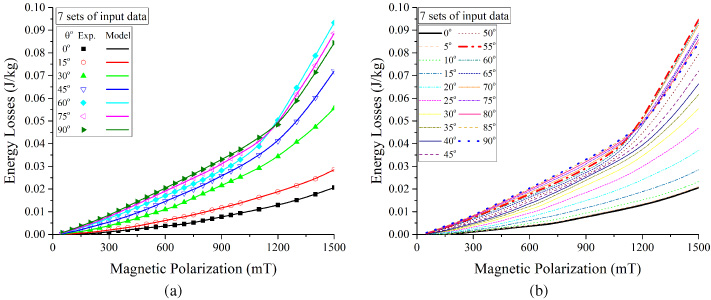
4.2. Model verification for power losses

An important parameter for the magnetic circuit designers is the dependence between energy losses and magnetic polarization. Based on the analysis, which was done in Subsection 4.1, the model with 7 sets of input data was chosen. Under this condition, in order to validate the application of the proposed model, the energy loss variation as a function of J was reconstructed based on Eq. (1) for 19 values of angle θ, between 0° and 90°, with a step of 5°.

Figures 5, 6, and 7 show the dependencies W (J) in the case of mechanical, laser and electro-erosion cut samples. The computed data were determined with an equation similar to Eq. (2), obtained by replacing parameter H ₀ with an imposed J ₀ value.

Fig. 5.

Energy loss variations as a function of the magnetic polarization, determined in the case of samples cut through mechanical punching: (a) experimental and computed values (symbol – experimental, full line – computed); (b) predicted values for 19 angles ranging from 0° to 90°.

Fig. 6.

Energy loss variations as a function of the magnetic polarization, determined in the case of samples cut through laser technology: (a) experimental and computed values (symbol – experimental, full line – computed); (b) predicted values for 19 angles ranging from 0° to 90°.

Energy loss measurements offer a high-quality description of the averaged material behavior, because the grains and the Goss texture characteristics in the entire strip volume are taken into consideration. In all the cases the computation leads to very good results even in the low magnetic field region. The model is a general one and it can be successfully applied for energy loss computation.

Fig. 7.

Energy loss variations as a function of the magnetic polarization, determined in the case of samples cut through electro-erosion procedure: (a) experimental and computed values (symbol – experimental, full line – computed); (b) predicted values for 19 angles ranging from 0° to 90°.

Disregarding the cutting procedure, the easy magnetization axis that imposes the lowest values of energy losses, is associated with the sample cut parallel with the RD, for which it can be noticed the shift of hard magnetization axis from 90° cut sample, in the low magnetic polarization region, to 60° (Figs 5.a, 6.a and 7.a) or 55° (Figs 5.b, 6.b and 7.b), for the high magnetic induction zone. The hard magnetization axis is characterized by the highest values of the energy losses. For laser technology, due to the induced thermal stresses, an increase of energy losses is observed. In the case of predicted values (Fig. 6.b) for the 19 angles’ case, a shift of the hard magnetization axis from 55° to 65°, with respect to the RD, is present. In good agreement with literature [4,16–22], for the mechanical and electro-erosion technologies’ analysis, the predicted behavior puts in evidence the presence of the easy axis at 0° and of the hard axis at 90° or 55°, at low and, respectively, high values of the excitation.

5. Conclusions

The proposed model which uses as input 7 sets of experimental data, based on ODF theory, predicts with an increased degree of accuracy the normal magnetization curve and the energy losses in the case of M-0H steel. The original model, based on three parameters, has a low accuracy in the low magnetic field region, fact that makes it inadequate for a precision electric transformer design. The normal magnetization curves and energy losses could be predicted for any angle θ from 0° to 90°, based on experimental measurements obtained in the case of samples cut at 0, 15, 30, 45, 60, 75 and 90 degrees with respect to the rolling direction.

Footnotes

Acknowledgements

The work of V. Manescu (Paltanea), G. Paltanea and P.C. Andrei has been funded by U.P.B., through “Excellence Research Grants” Program, UPB-GEX 2017. Identifier: UPB-GEX2017, Ctr. No. 04/25.09.2017 (OPTIM-IE4), Ctr. No. 02/25.09.2017 (ANIZ-GO) and Ctr. No. 06/25.09.2017 (STATIC-BH). The work of H. Gavrila has been funded by a grant of CNCS/CCCDI – UEFISCDI, Project Number 10PTE/2016, within PNCDI III “Brushless servo-motors series utilizing soft magnetic composite materials”. The samples involved in the study were provided by ELECTROPUTERE Power Transformers, 80 Calea Bucuresti, 200440, Craiova, Romania.

References

Fiorillo

Dupre

L.R.

Appino

and Rietto

A.M.

, Comprehensive model of magnetization curve hysteresis loops, and losses in any direction in grain-oriented Fe-Si, IEEE Trans. Magn. 38 (2002), 1467–1976, doi:10.1109/20.999119.

Nakata

Ishihara

Yamada

and Sasano

, Non linear analysis of rotating flux in the T-joint of a three-phase, three-limbed transformer core, in: Proc. Soft Magnetic Materials 2 Conf., Cardiff, 1975.

Benda

Bydzovsky

and Usak

, Combined influence of shape and magnetocrystalline anisotropy on measured magnetization curves of Si-Fe sheets, J. Phys. IV 8 (1998), 627–630, doi:10.1051/jp4:19982145.

Nencib

Spornic

Kedous-Lebouc

and Cornut

, Macroscopic anisotropy characterization of Si-Fe using a rotational single sheet tester, IEEE Trans. Magn. 31 (1995), 4047–4049, doi:10.1109/20.489857.

Higuchi

Nakao

Takahashi

Tokumasu

Fujiwara

and Ishihara

, Modeling of two-dimensional magnetic properties based on one-dimensional magnetic measurements, IEEE Trans. Magn. 48 (2012), 3486–3489, doi:10.1109/TMAG.2012.2198878.

Chwastek

, Anisotropic properties of non-oriented steel sheets, IET Electric Power Applications 7 (2013), 575–579, doi:10.1049/iet-epa.2013.0087.

Culity

B.D.

and Graham

C.D.

, Introduction to Magnetic Materials, 2nd edn, Wiley-IEEE Press, 2008.

Demian

Cassoret

Brudny

J.F.

and Belgrand

, AC magnetic circuits using nonsegmented shifted grain oriented electrical steel sheets: Impact on induction machine magnetic noise, IEEE Trans. Magn. 48 (2012), 1409–1412, doi:10.1109/TMAG.2011.2174146.

Pfützner

Mulasalihovic

Yamaguchi

Sabic

Shilyashki

and Hofbauer

, Rotational magnetization in transformer cores—A review, IEEE Trans. Magn. 47 (2011), 4523–4533, doi:10.1109/TMAG.2011.2151201.

10.

Kulkarni

S.V.

and Khaparde

S.A.

, Transformer Engineering: Design and Practice, Marcel Dekker, New York, USA, 2004.

11.

Lanotte

Luponio

De Iorio

Tagliaferri

and Tammaro

, Effect of laser cutting on magnetic properties of grain-oriented Fe-Si ribbons, J. Sci. Technol. 8 (1992), 252–256, doi:10.1179/mst.1992.8.3.252.

12.

Manescu (Paltanea)

Paltanea

Gavrila

and Nicolaide

, Analysis of the cutting area obtained through mechanical and electrical discharge technologies in non oriented silicon iron sheets, Rev. Roum. Sci. Tech-El. 60 (2015), 143–152.

13.

Bunge

H.J.

, Fifty years texture in research and practice, Texture and Microstructure (1988), 55–75, doi:10.1155/TSM.8-9.55.

14.

Chwastek

Baghel

A.P.S.

de Campos

M.F.

Kulkarni

S.V.

and Szczygowski

, A description of magnetic properties of grain-oriented steels, IEEE Trans. Magn. 51 (2015), 6000905, doi:10.1109/TMAG.2015.2449775.

15.

Bunge

H.J.

, Symmetries in texture analysis, Acta Cryst. 41 (1985), 59–67, doi:10.1107/S0108767385000101.

16.

Pluta

W.A.

, Angular properties of specific total loss component under axial magnetization in grain-oriented electrical steel, IEEE Trans. Magn. 52 (2016), 6300912, doi:10.1109/TMAG.2015.2496547.

17.

Pluta

W.A.

, Specific total loss components under axial magnetization in electrical steel sheets with different degree of Goss texture, IEEE Trans. Magn. 44 (2008), 3832–3835, doi:10.1109/TMAG.2008.2002190.

18.

Pluta

W. A.

, Some properties of factors of specific total loss components in electrical steel, IEEE Trans. Magn. 46 (2010), 322–325, doi:10.1109/TMAG.2009.2033559.

19.

Bunge

H.J.

, Texture Analysis in Materials Science – Mathematical Methods, Butterworths, London, 1982.

20.

Bunge

H.J.

, Advances and Applications of Quantitative Texture Analysis Bunge

H.J.

and Esling

(eds), Clausthal, FRG, 1989. Oberursel, FRG. DGM Informationsgesellschaft – Verlag, 1991, pp. 3–18.

21.

Jiang

Rossi

and Parent

, Anisotropy model for modern grain oriented electrical steel based on orientation distribution function, AIP Advance 8 (2018), 056104, doi:10.1063/1.5006471.

22.

de Campos

M.F.

, Anisotropy of steel sheets and consequence for Epstein test: I theory, in: Proc. 28th IMEKO World Congr., 2006, pp. 1–6.

23.

Soinski

, The anisotropy of coercive force in cold-rolled Goss texture electrical sheets, IEEE Trans. Magn. 23 (1987), 3878–3881, doi:10.1109/TMAG.1987.1065769.

24.

de Campos

M.F.

Landgraf

F.J.G.

and Tschiptschin

A.P.

, A metod to estimate magnetic induction from texture in non-oriented electrical steels, J. Magn. Magn. Mater. 226-230 (2001), 1536–1538, doi:10.1016/S0304-8853(01)00027-0.

25.

Paltanea

Gavriă

Popovici

and Ionescu

, Magnetic anisotropy in grain oriented steels cut through mechanical punching and electro-erosion technologies, in: AIP Conference Proceedings, Vol. 1809, 2017, p. UNSP020042, doi:10.1063/1.4975457.

26.

Paltanea

and Gavriă

, Magnetic anisotropy in silicon iron alloys, Electrical and Electronic Engineering 2 (2012), 383–388, doi:10.5923/j.eee.20120206.07.

27.

Baudouin

Wulf

M.D.

Kestens

and Houbaert

, The effect of the guillotine clearance on the magnetic properties of electrical steel, J. Magn. Magn. Mater. 256 (2003), 32–40, doi:10.1016/S0304-8853(02)00004-5.

28.

Baudouin

Belhadj

and Houbaert

, Effect of the rapid heating on the magnetic properties of non-oriented electrical Steels, J. Magn. Magn. Mater. 238 (2002), 221–225, doi:10.1016/S0304-8853(01)00916-7.

29.

Appino

Hamrit

Fiorillo

Ragusa

de la Barrière

Mazaleyrat

and LoBue

, Skin effect in steel sheets under rotating induction, Int. J. Appl. Electromagn. Mech. 48 (2015), 247–254, doi:10.3233/JAE-151995.

30.

Appino

Ferrara

Fiorillo

, International comparison on SST and Epstein measurements in grain-oriented Fe-Si sheet steel, Int. J. Appl. Electromagn. Mech. 48 (2015), 123–133, doi:10.3233/JAE-151978.

31.

Pfutzner

Shilyashki

and Mulasalihovic

, Modern transformer cores – 3 – dimensional magnetic systems of under-estimated complexity, Int. J. Appl. Electromagn. Mech. 48 (2015), 143–151, doi:10.3233/JAE-151980.

32.

Yamamoto

Hamada

and Yanase

, Effects of compressive stress normal to the surface of grain-oriented electrical steel sheets, Int. J. Appl. Electromagn. Mech. 48 (2015), 153–158, doi:10.3233/JAE-151981.