A mathematical modelling and experimental study of annular-radial type magnetorheological damper

Abstract

An experimental study was undertaken to evaluate the mathematical modelling of the magnetorheological (MR) damper featuring annular radial gap on its valve. The experiment was conducted using a fatigue dynamic test machine under particular excitation frequency and amplitude to get force-velocity and force-displament characteristics. Meanwhile, the mathematical modelling was done using quasi-steady modelling approach. Simulation using adaptive neuro fuzzy inference (ANFIS) Algorithm (Gaussian and Generalized Bell) were also carried out to portray the damping force-displacement modelling that is used to compare with the experimental results. The experimental characteristics show that amplitudes excitation and current input affect the result damping force value. The comparison of the experimental and mathematical results presented in this paper shows a significant difference in damping force value and that the quasi-steady modelling could not significantly approach the damping force-velocity results. Moreover, the semi-active damper is compared to the passive damper. The results show that a semi-active damper performs better than a passive damper because it only requires a little power. Based on the damping force-displacement modelling, it can be seen that Gaussian has a higher accuracy rather than Generalized Bell. Discussion on the energy dissipation and equivalent damping coefficient were also accomodated in this paper. Having completed in mathematical modelling and simulation, the damper would be ready for further work in-vehicle application that is development of control system.

Keywords

MR damper annular-radial MR valve quasi-steady modelling MR damper characteristics energy dissipated ANFIS Algorithm

1. Introduction

A smart material based on magnetic is a material that outside stimuli can be interfered with magnetic fields. There are several types of smart material based on magnetic – for example, magnetorheological (MR) fluids, MR greases, MR Foam, MR plastomers and MR elastomers [1,2]. An MR fluid is a material consisted of magnetic particles carried in a fluid that can be interfered with by a magnetic field resulting in reversible intrinsic properties [3–7]. Because the rheological properties of an MR fluid can be changed drastically when a magnetic field is applied, this fluid has been used and developed in various devices [8,9]. Its applications include shock absorbers (MR dampers), clutches (MR clutches) [10] and brakes (MR brakes) [11]. An MR damper is an example of a semi-active device that can be used for suspension systems. Lately, semi-active suspensions are being developed by many researchers because they perform better than passive suspensions. A semi-active suspension can be fully controlled on any terrain or in any road conditions, while a passive suspension can only be used in certain road conditions [12].

MR dampers have been studied a lot lately [13–16]. An MR damper is a semi-active device that contains an MR fluid, and its properties change if it is exposed to a magnetic field. The development of fluids that can be controlled began in the late 1940s, according to Spencer [17]. The viscosity of MR fluids can be changed by supplying current input into the electromagnetic coil, which can produce a real-time variable damping system.

An MR damper is a promising semi-active suspension system for automotive industries because it produces a damping force that can be varied by requiring only a small amount of power [18,19]. In the last decades, MR dampers have been successfully applied in some automotive industries. The Chevrolet Corvette and Cadillac XLR were the first vehicles to use magnetic ride control, a magnetic-fluid-based real-time damping suspension system. The four-wheel displacement sensor is used on the body of the car, measuring the motion of the wheels on the road surface. Thus, the damper can respond and adjust in almost one millisecond [20].

The main component that considerably affects an MR damper’s performance is the MR valve [21]. Both annular and radial types of MR valves have been developed. Abd Fatah [22] and Idris [23] introduced an MR valve using the serpentine flux path method; the combination of the arrangement of magnetic and nonmagnetic components is able to manipulate the magnetic flux flow path. Imaduddin [24,25] developed a meandering flow path structure consisting of multiple annular and radial gaps. The results of the study show a significant improvement in the pressure drop value. A meandering flow path structure was also developed by Ichwan [26]. The study demonstrates that changing the number of module stages can modify the pressure drop rating. Recently, Wirawan [27] developed an MR valve for an upside-down damper, designed with two annular gaps and one radial gap, and operated with a flow mode. In the study, a magnetic flux simulation and pressure drop were performed using mathematical predictions, showing a better result than that of active and passive suspensions.

An MR damper works in a mechanical structure, and its damping force can be adjusted in real-time conditions. A variation of the current input passing through the wire in the MR damper is used for the real-time adjustment [28]. The numerical simulation [29,30] and experiment [31,32] were conducted to study its characteristics. The development of models that accurately describe MR damper behaviour needs to be developed to evaluate the benefits of an MR damper as a vibration controller. The development of analytic, parametric [33] and non-parametric models were carried out to portray MR damper behaviour that has been observed. Wang [34] proposed an asymmetric MR damper analytical model, which can effectively illustrate the hysterical characterization of the damping force and piston velocity, although some deviations are found. The phenomenological parametric model developed by Spencer [17] can accurately portray MR damper responses to random and cyclic excitations for variable and constant magnetic fields. Fuzzy logic and neural network computing models were used to portray MR damper behaviour. Few studies have evaluated an experimental study of an MR damper; most of them have assessed an MR damper using a numerical simulation. Recently, Ubaidillah [20] proposed a sixth-order polynomial model to generate MR damper hysteresis behaviour under harmonic excitations, and compared the proposed model with experimental results. Imaduddin [33] proposed an experimental study and LuGre’s parametric modelling of an MR valve with multiple radial and annular gaps. It was concluded that the parametric model could approach the hysteresis model when it becomes vulnerable to certain excitation frequencies. Hu [35] proposed MR damper characteristics using the Simulink tool under the sine excitation and evaluated the damping force characteristics of the MR damper with the prediction results.

Since the experimental results and damping force predictions were not provided by Wirawan [27], therefore, the purpose of this study is to continue the MR damper characterization and evaluate its accuracy of the damping force value of the mathematical modelling. The MR damper experimental results are observed in terms of the characteristics of damping force versus the displacement of the piston, and damping force versus the velocity of the piston. The peak value of the damping force versus piston velocity characteristics will be evaluated with the results of the damping force using mathematical modelling. Furthermore, this study will not only discuss the damping force versus displacement modelling of Gaussian and Generalized Bell but also the equivalent damping coefficients and energy dissipated.

2. Materials and methods

2.1. Materials

The details of the MR damper design are presented in the previous literature by Wirawan [27]. The designed MR damper is a prototype of the MR Damper that is made according to specifications for Daihatsu Terios cars. Figure 1 shows the configuration of the MR damper used for this experimental study. The MR damper is a mono-tube MR damper with flow mode operation. Figure 2 shows the six parts of the MR valve. Both the lower and upper cases are made from aluminium. The piston rod is attached to the inner valve, while the outer valve is attached to the upper case. In the middle of the inner and outer valve, there is an aluminium bobbin and 28 AWG copper wire.

Fig. 1.

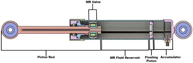
MR damper configuration.

Fig. 2.

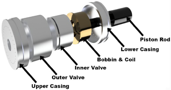
Exploded view of the MR valve.

Fig. 3.

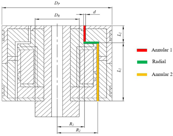
MR valve parameters.

2.2. Methods

2.2.1. Magnetic simulation

The Finite Element Method Magnetics (FEMM) 4.2 software was used in previous literature by Ichwan [26] that also was used in this study. The simulation provides magnetics flux density along the MR fluid flow path. The problem to be simulated was the magnetic problem with the axisymmetric setting.

Figure 3 shows the MR valve parameters, while Table 1 shows the parameter values. These parameters were used for both the FEMM simulation and the mathematical modelling. The simulation was conducted with various current inputs, namely 0.25, 0.5 and 0.75 A. The design parameters were chosen based on the design limitation of the piston space being used for the Daihatsu Terios cars. This was considered by the total stroke of the MR damper. Moreover, the initial dimensions of the MR valve located in effective dimensions of annular and radial gaps. Based on the maximum space of piston thickness, the annular and radial area were divided into proportional dimensions. This had been considered to aim the serpentine model. Furthermore, the consideration of the dimensions were also determined by the manufacturability factor.

Table 1
MR valve parameters

Parameter Description Value Unit

D _P Piston diameter 50 mm

D _R Piston rod diameter 20 mm

d Flow gap 1 mm

R ₁ Annular 1 radius 12.5 mm

R ₂ Annular 2 radius 18.5 mm

L ₁ Annular 1 length 8.5 mm

L ₂ Annular 2 length 29 mm

d _c Coil diameter 28 AWG

l Coil length 17 mm

r ₁ Inner coil radius 10.5 mm

r ₂ Outer coil radius 16.5 mm

N Number of coil turns 350 turns

L ₀ Orifice gap length 1.5 mm

R ₀ Orifice radius radial 18.5 mm

𝜂(MRF 132-DG) Fluid viscosity 0.112 Pa-s

Parameter	Description	Value	Unit
D _P	Piston diameter	50	mm
D _R	Piston rod diameter	20	mm
d	Flow gap	1	mm
R ₁	Annular 1 radius	12.5	mm
R ₂	Annular 2 radius	18.5	mm
L ₁	Annular 1 length	8.5	mm
L ₂	Annular 2 length	29	mm
d _c	Coil diameter	28	AWG
l	Coil length	17	mm
r ₁	Inner coil radius	10.5	mm
r ₂	Outer coil radius	16.5	mm
N	Number of coil turns	350	turns
L ₀	Orifice gap length	1.5	mm
R ₀	Orifice radius radial	18.5	mm
𝜂(MRF 132-DG)	Fluid viscosity	0.112	Pa-s

The magnetic flux density was used to calculate the MR fluid yield stress. Each area of the valve has a different MR fluid yield stress depending on the value of the magnetic flux density of each zone. Fluid flow gap classification was used to simplify the calculation of yield stress for each zone. It was divided into three zones: annular, radial and orifice.

2.2.2. Quasi-steady modelling

The quasi-steady modelling was done to obtain the predicted value of the damping force. It was done at certain speed values of piston displacement. Damping force can be obtained in compression and rebound conditions using Eq. (1). $\begin{eqnarray}\displaystyle F_{d}={\rm\Delta}PA & & \displaystyle\end{eqnarray}$ (1) where F _d is the damping force, ΔP is the pressure drop, and A is the valve surface area under two different conditions: jounce (MR damper in compression conditions) and rebound (MR damper in rebound conditions). The expressions of the surface area are shown in Eqs (2) and (3), $\begin{eqnarray}\displaystyle \text{} & \text{} & \displaystyle A_{c}=\frac{1}{4}{\pi}D_{p}^{2}\end{eqnarray}$ (2) $\begin{eqnarray}\displaystyle \text{} & \text{} & \displaystyle A_{r}=\frac{1}{4}{\pi}(D_{p}^{2}-D_{r}^{2})\end{eqnarray}$ (3) where A _c is the surface area of the compression condition, A _r is the surface area of the rebound condition, D _p is the valve diameter, and D _r is the piston rod diameter.

The total value of the pressure drops is expressed in Eq. (4). Using Eqs (5) to (9) [26], the pressure drops are divided into three types: viscous, yield and orifice. A viscous pressure drop is used to calculate a pressure drop in off-state conditions because it is only obtained from the MR fluid viscosity value, so there is no magnetic field induction process. On-state conditions pressure drop use the yield pressure drop equation because the creation of electromagnetic fields from electric currents induced into the coil affects MR fluid yield stress. $\begin{eqnarray}\displaystyle \text{} & \text{} & \displaystyle {\rm\Delta}P={\rm\Delta}P_{\mathit{viscous}}+{\rm\Delta}P_{\mathit{yield}}+{\rm\Delta}P_{\mathit{orifice}}\end{eqnarray}$ (4) $\begin{eqnarray}\displaystyle \text{} & \text{} & \displaystyle {\rm\Delta}P_{\mathit{viscous},\mathit{annular}}=\frac{6{\eta}QL}{{\pi}d^{3}R}\end{eqnarray}$ (5) $\begin{eqnarray}\displaystyle \text{} & \text{} & \displaystyle {\rm\Delta}P_{\mathit{viscous},\mathit{radial}}=\frac{6{\eta}Q}{{\pi}d^{3}}\ln \left(\frac{R_{2}}{R_{1}}\right)\end{eqnarray}$ (6) $\begin{eqnarray}\displaystyle \text{} & \text{} & \displaystyle {\rm\Delta}P_{\mathit{yield},\mathit{annular}}=\frac{c{\tau}_{y}(B)L}{d}\end{eqnarray}$ (7) $\begin{eqnarray}\displaystyle \text{} & \text{} & \displaystyle {\rm\Delta}P_{\mathit{yield},\mathit{radial}}=\frac{c{\tau}_{y}(B)}{d}(R_{2}-R_{1})\end{eqnarray}$ (8) $\begin{eqnarray}\displaystyle \text{} & \text{} & \displaystyle {\rm\Delta}P_{\mathit{orifice}}=\frac{8{\eta}QL_{0}}{{\pi}R_{0}^{4}}\end{eqnarray}$ (9) where 𝜂 is fluid viscosity, Q is the fluid flow rate, L is the annular gap length, R ₂ is the outer gap radius, R ₁ is the inner gap radius, L ₀ is the orifice gap length, R ₀ is the orifice radius radial, d is the flow gap diameter, τ_y(B) is yield stress and c as the flow coefficient.

The fluid flow rates, Q, and flow function coefficient, c, can be obtained using Eqs (10) and (11), $\begin{eqnarray}\displaystyle \text{} & \text{} & \displaystyle Q=\frac{{\pi}d^{2}v}{4}\end{eqnarray}$ (10) $\begin{eqnarray}\displaystyle \text{} & \text{} & \displaystyle c=2.07+\frac{12Q{\eta}}{12Q{\eta}+0.8{\pi}Rd^{2}{\tau}(B)}\end{eqnarray}$ (11) where v is the piston rod speed and c is the flow function coefficient. Meanwhile, yield stress, τ_y(B), can be approximated by the polynomial equation expressed in Eq. (12), $\begin{eqnarray}\displaystyle \begin{array}{@{}l@{}}{\tau}_{y}(B)=-58.92B^{3}+74.66B^{2}+35.74B-3.387,\quad \text{for }{\tau}_{y}(B)>0\\ {\tau}_{y}(B)=0,\quad \text{for }{\tau}_{y}(B)<0\end{array} & & \displaystyle\end{eqnarray}$ (12) where τ_y(B) is MR fluid yield stress and B is the magnetic flux density.

2.2.3. Blackbox modelling

There are three inputs to generate the damping force prediction which are current input, displacement and velocity. Gaussian and Generalized Bell formula in the first layer were used to obtain the premise parameters that is shown in Eq. (13) and Eq. (14), $\begin{eqnarray}\displaystyle \text{} & \text{} & \displaystyle f(l,d,v)=e^{-\frac{(x-ci)}{2{\sigma}i^{2}}}\end{eqnarray}$ (13) $\begin{eqnarray}\displaystyle \text{} & \text{} & \displaystyle f(l,d,v)=\frac{1}{1+\left|{\displaystyle \frac{x-c}{a}}\right|^{2b}}\end{eqnarray}$ (14) where f (l, d, v) is the first layer output as function of current input, displacement or velocity, while σi, ci, a, b, c are premise parameters.

The second layer can be calculated using Eq. (15) with AND rules. $\begin{eqnarray}\displaystyle O2,i=wi=fi(I)\times fi(d)\times fi(v) & & \displaystyle\end{eqnarray}$ (15) where fi (I), fi (d) and fi (v) are the output for the current input, the displacement input and the velocity input, respectively.

Equation (16) shows the output from the third layer which is the multiplied average between each input being divided by the number of nodes, while Eq. (17) shows the output from the fourth layer. $\begin{eqnarray}\displaystyle \text{} & \text{} & \displaystyle O3,i=\overline{w{\iota}}=\frac{wi}{\displaystyle \mathop{\sum }_{i=1}^{n}wi}\end{eqnarray}$ (16) $\begin{eqnarray}\displaystyle \text{} & \text{} & \displaystyle O4,i=\overline{w{\iota}}gi=\overline{w{\iota}}(pi(I)+qi(d)+ri(v)+si)\end{eqnarray}$ (17) where w𝜄 is the relative rule weight of the i node, while pi, qi, ri and si are consequent parameters values after the completion of training process. However, pi = qi = ri are assumed to be 0. Furthermore, S1 (gi = si) is the representation of the fourth layer’s consequent parameters. Thus, Eq. (18) represents the final output from the fourth layer. $\begin{eqnarray}\displaystyle O4,i=\overline{w{\iota}}gi=\overline{w{\iota}}(si). & & \displaystyle\end{eqnarray}$ (18)

The final output which is fifth layer can be seen in Eq. (19), $\begin{eqnarray}\displaystyle O5,i=\mathop{\sum }_{i=1}^{n}\overline{w{\iota}}gi=\frac{\displaystyle \mathop{\sum }_{i=1}^{n}\overline{w{\iota}}(si)}{\displaystyle \mathop{\sum }_{i=1}^{n}wi}. & & \displaystyle\end{eqnarray}$ (19)

RMSE is used to calculate the value of relative error of the ANFIS modelling as shown in Eq. (20), $\begin{eqnarray}\displaystyle RMSE=\sqrt{\frac{1}{n}}\sum (\overline{Zt}-Z)^{2} & & \displaystyle\end{eqnarray}$ (20) where n is the total number of testing sets, Zt is the experimental value of damping force and Z is the value of damping force prediction.

2.2.4. Experimental setup

The experiment was carried out in the Solid Mechanics Laboratory at Universiti Teknologi Malaysia using a fatigue dynamic test machine. This machine consists of four main components: the Shimadzu Servopulser EHF-L Series, the Shimadzu 4830 Controller Servopulser control unit, a PC unit and a power supply. The Shimadzu Servopulser has two sensors: a load cell sensor and a position sensor. The Shimadzu Servopulser EHF-L Series is connected to the 4830 Controller Servopulser control unit, which receives measurement data from the Shimadzu engine sensors and stores it on the host PC through the 4830 Servo Controller software. The power supply is needed to perform the experiment in an on-state condition and is connected to the coil of the MR damper to conduct an electric current. The experiment was conducted with a constant frequency of 2 Hz. Each frequency was performed with 0.004, 0.008, 0.010, 0.012 and 0.016 m amplitudes. These amplitudes were applied in several current input variations, namely 0.25, 0.5 and 0.75 A. Figure 4 shows the configuration of the MR damper experiment for this study.

Fig. 4.

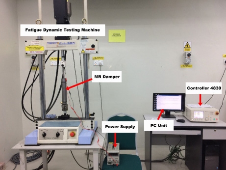
Experimental configuration.

2.2.5. Energy dissipated & equivalent damping coefficient

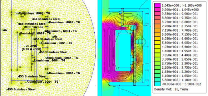
To compare the MR damper damping performance with the passive viscous damper, it is important to determine the energy dissipated in the full cycle by equalizing the equivalent damping coefficient [36,37]. The equation of energy dissipated in the full cycle is shown in Eq. (21), $\begin{eqnarray}\displaystyle W_{mr}=\int _{0}^{2{\pi}/{\omega}_{d}}F_{mr}dx=\int _{0}^{2{\pi}/{\omega}_{d}}C_{eq}{\dot{x}}dx & & \displaystyle\end{eqnarray}$ (21) where ω_d is the frequency of actuation of the sinusoidal excitation, ${\dot{x}}$ is the relative damper velocity, F _mr is the damping force, W _mr is the energy dissipated and C _eq is the equivalent damping coefficient.

Fig. 5.

Meshing results of the 2D MR valve design and the results of the magnetic flux density at 0.75 A current input.

Fig. 6.

The magnetic flux density throughout the fluid flow path.

With the assumption that a simple harmonic excitation, x = Xsinω_d t, is used in Eq. (22), where X is the excitation amplitude, Eq. (22) becomes Eq. (23), $\begin{eqnarray}\displaystyle W_{mr} & = & \displaystyle \int _{0}^{2{\pi}/{\omega}_{d}}C_{eq}({\dot{x}})^{2}dx\nonumber\\ \displaystyle & = & \displaystyle \int _{0}^{2{\pi}/{\omega}_{d}}C_{eq}({\omega}_{d}X\cos {\omega}_{d}t)^{2}dx\nonumber\\ \displaystyle & = & \displaystyle {\pi}C_{eq}{\omega}_{d}X^{2}.\end{eqnarray}$ (22) Therefore, C _eq can be formulated as, $\begin{eqnarray}\displaystyle C_{eq}=\frac{W_{mr}}{{\pi}{\omega}_{d}X^{2}}. & & \displaystyle\end{eqnarray}$ (23)

3. Results and discussion

3.1. Magnetic simulation results

The simulation using FEMM 4.2 software provides the magnetic flux density values, as shown in Fig. 5. In the meshing section, there is a configuration of the material used in the area around the MR valve. The material consists of aluminium as a diamagnetic material and stainless steel as a magnetic property material. In addition, MRF 132 DG from Lord Corporation was used for the fluid properties, along with 28 AWG coil with 350 turns. The simulation performed with various current inputs, namely 0.25, 0.5 and 0.75 A. The meshing model is a triangular element with a total of 11591 nodes. The results of the magnetic simulation show that the current input affects the magnetic flux density value. The power that is needed for a 0.75 A current input is 19.91 W.

Figure 6 shows the magnetic flux density along with the fluid flow path. The magnetic flux density is divided into three zones: the first annular zone, the radial zone and the second annular zone. The first-largest magnetic flux density, 0.22 Tesla at 0.75 A, is in the first annular zone; the second-largest magnetic flux density, 0.21 Tesla at 0.75 A, is in the second annular zone.

Fig. 7.

Damping force-displacement caracteristics at 2 Hz frequency under different excitation amplitude at a constant current input (a) 0 A, (b) 0.25 A, (c) 0.5 A and (d) 0.75 A.

3.2. Experimental results

The experiment provides data to make MR damper characteristics. Figure 7 shows the graphs of the MR damper characteristics, namely the relationship between damping force and displacement at the frequency of 2 Hz at current inputs of 0, 0.25, 0.5 and 0.75 A under different excitation amplitudes. The different excitation amplitudes increase the value of different damping forces. Furthermore, the characteristics of the damping force and velocity at the frequency of 2 Hz under different excitation amplitudes at different constant current inputs can be seen in Fig. 8. These results show that the application of different current inputs and amplitudes cause differences in the damping force value. When a larger amplitude is applied, the damping force value increases. The minimum damping force value is at 0 A, while the maximum damping force value is at 0.75 A. There are graphs with overlapping values at a frequency of 2 Hz in Fig. 8(b), (c) and (d).

Fig. 8.

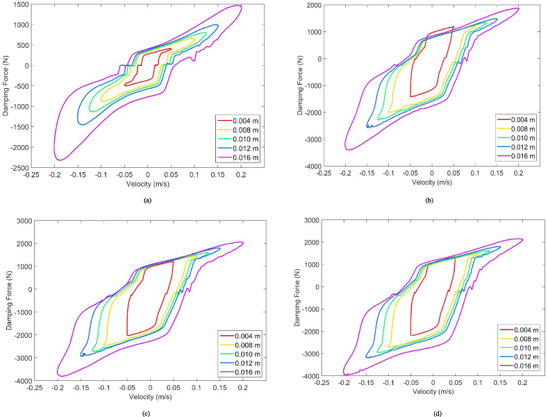
Damping force-velocity caracteristics at 2 Hz frequency and under different excitation amplitude at a constant current input (a) 0 A, (b) 0.25 A, (c) 0.5 A and (d) 0.75 A.

3.3. Benchmarking between prediction and experiment

The damping force prediction results were obtained from Eq. (1). The experiment was done by collecting the peak value from the graph of the relationship between damping force and velocity obtained from the sinusoidal input for the data points. The comparison between the result of mathematical modelling and the MR damper experiment at 2 Hz frequency is presented in Fig. 9. The higher magnetic field is applied, the higher damping force that is produced. It is clearly seen that the damping force at 0.25 A is higher than 0 A. The negative position in the coordinate only shows the representation of rebound condition of the MR damper, while the positive position shows the representation of compression condition of MR damper. The negative and positive position in the coordinate are not connected to the actual values of the damping force, so it is only to distinguish the compression and rebound condition of the MR damper, for example, based on Fig. 9 the experimental result of the damping force at 0 A and 0.2 m/s is about 2000 N for compression condition, while the rebound condition is around 1500 N. Meanwhile, the damping force value at 0.25 A and 0.2 m/s is about 3000 N for compression condition, while the rebound condition is around 1900 N. Thus, it is clear that the damping force value for compression condition (in coordinate is at positive position) at 0.25 A (3000 N) is higher than at 0 A (2000 N). Moreover, the damping force value for rebound condition at 0.25 A (3000 N) is higher than at 0 A (2000 N). The biggest damping force value of mathematical modelling, which is 2432.235 N for compression and 1976.897 N for rebound; the biggest damping force value of experimental results is 3791.514 N for compression and 2101.968 N for rebound. In addition, the damping force value of mathematical modelling at the current input 0 and 0.25 A has the same results. This is due to the small value of the magnetic flux density that was generated at a 0.25 A current input, which affects the small value of the pressure drop to calculate the value of the damping force. Figure 9 also shows that the difference of the comparison results is quite big, with the relative error value around 5.9% to 85.9%.

Fig. 9.

Damping force comparison between mathematical modelling results and experimental results at a frequency of 2 Hz.

3.4. Benchmarking between passive damper and semi-active damper

The benchmarking is to compare the Daihatsu Terios car damping force as a passive damper and damping force results of the semi-active damper using the mathematical modelling and experiment of the MR damper that is proposed in this study. This can be seen in Fig. 10. There are no significant value changes in the passive damper damping force compared to the semi-active damper. The damping force prediction calculation results show that the off-state damping force is higher than the passive damper damping force, while the damping force with a maximum input current voltage at 0.75 A is higher than the passive damper damping force. These show that the semi-active damper can be more beneficial than the passive damper, with the semi-active damper very effective when used at high speeds and very beneficial if the car hits a bump.

Fig. 10.

Damping force comparison between the passive damper and semi-active damper at a frequency of 2 Hz.

3.5. Blackbox modelling

Two membership functions of ANFIS were used to model the MR damper. The used configurations were 3-5-6 and the number of epochs was 2500. The prediction results of damping force versus displacement are compared with the experimental results of damping force versus displacement that is shown in Fig. 11. The predicted results of Gaussian and Generalized Bell have a big difference with the experimental results. This is because of the high number of the training error value. However, Gaussian and Generalized Bell modelling are able to portray the value of predicted damping force.

Fig. 11.

The comparison of damping force-displacement modelling and experiment at a constant amplitude (a) 4 mm, (b) 8 mm, (c) 10 mm, (d) 12 mm and (e) 16 mm.

Table 2 illustrates the relative error of the ANFIS training data. In general, the relative error of Gaussian is higher than Generalized Bell. This shows that the accuracy of Gaussian is higher than Generalized Bell.

Table 2

Relative error value of Gaussian and Generalized Bell modelling

	Relative error of Gaussian (%)				Relative error of Generalized Bell (%)
Amplitude	0 A	0.25 A	0.5 A	0.75 A	0 A	0.25 A	0.5 A	0.75 A
4 mm	26.55	20.19	27.54	33.15	25.28	15.93	22.63	27.77
8 mm	19.93	32.88	39.94	41.52	19.49	26.84	23.21	22.54
10 mm	35.32	37.14	37.13	38.25	22.67	32.35	28.56	27.58
12 mm	27.94	36.60	37.54	39	29.62	40.77	33.68	33.60
16 mm	45.85	52.08	57.82	62.09	46.89	52.26	46.49	45.07
Average	31.12	35.78	39.99	42.80	28.79	33.63	30.91	31.31

3.6. Energy dissipated & equivalent damping coefficient results

Figures 12 and 13 show the equivalent damping coefficient under different current inputs and excitation amplitudes. The results of the equivalent damping coefficient decrease as the excitation amplitude increases, which can be seen in Fig. 12. On the other hand, Fig. 13 shows that the equivalent damping coefficient increases as the current input increases.

The energy dissipated under different current inputs and excitation amplitudes are presented in Figs 14 and 15. Because of the larger hysteresis loop, the energy dissipated will increase with the increase of amplitude excitation, as shown in Fig. 14. However, Fig. 15 shows that the higher the current input, the higher the energy dissipated.

Fig. 12.

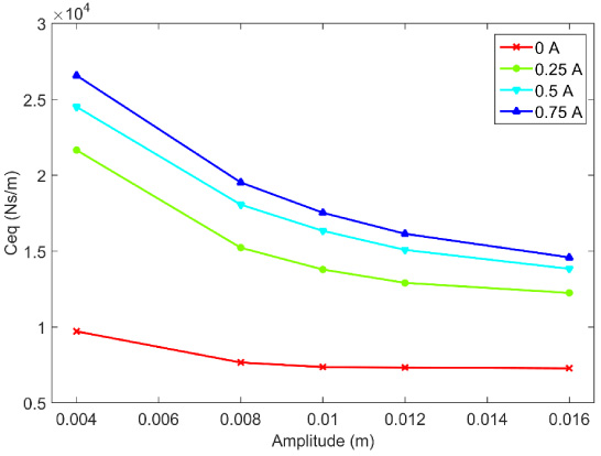
Relationship between equivalent damping coefficient and amplitude under various current input at a frequency of 2 Hz.

Fig. 13.

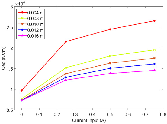
Relationship between equivalent damping coefficient and current input under various amplitude at a frequency of 2 Hz.

Fig. 14.

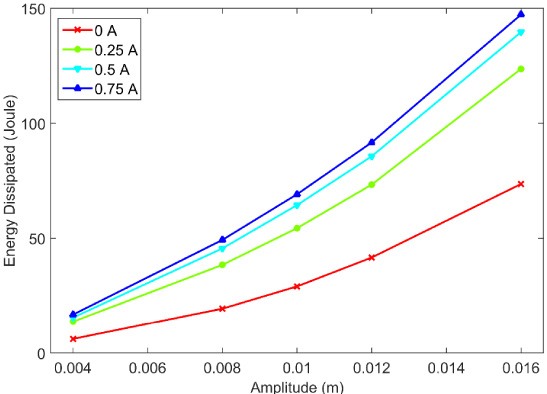
Relationship between energy dissipated and amplitude under various current input at a frequency of 2 Hz.

Fig. 15.

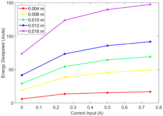
Relationship between energy dissipated and current input under various amplitude at a frequency of 2 Hz.

The energy dissipated divided by the amplitude squared, obtained from Eq. (22), is displayed in the graphs as a parabolic function. Thus, the energy dissipated increases linearly as the excitation amplitude increases, while the equivalent damping coefficient decreases linearly as the excitation amplitude increases.

4. Conclusion

The MR damper characteristics are shown in the graph on the relationship between damping force and displacement and in the graph on the relationship between damping force and velocity. From these graphs, it can be concluded that the higher the amplitude and current input, the higher the value of the damping force result. A comparison of the mathematical modelling and experimental results is presented in graphical form, showing that the value of damping force mathematical modelling with experimental results has a sufficiently big difference. It also shows that mathematical modelling could not approach the experimental results of the peak damping force value. It is because mathematical modelling shows a significant difference of the value of the peak damping force compared to experimental result. However, the value is still on the same pattern for both mathematical modelling and experimental result. The damping force of the semi-active damper performs better than that of the passive damper. Furthermore, the modelling results of ANFIS Algorithm have a big difference compared to the experimental results. In addition, the investigation results of the energy dissipated and equivalent damping coefficient regarding the excitation amplitude and current input show the opposite results: the higher the excitation amplitude in a current input is, the higher the energy dissipated is, but the equivalent damping coefficient value will decrease, and vice versa.

Footnotes

Acknowledgement

This research was funded by the Ministry of Research and Technology/BRIN of the Republic of Indonesia under Hibah WCR 2021.

References

Ubaidillah

Choi

H.J.

Mazlan

S.A.

Imaduddin

and Harjana

, Fabrication and viscoelastic characteristics of waste tire rubber based magnetorheological elastomer, Smart Mater. Struct. 25(11) (2016), 1–14.

Shabdin

, Material characterizations of gr-based magnetorheological elastomer for possible sensor applications: Rheological and resistivity properties, Materials (Basel) 12(3) (2019), 391.

Bin Pokaad

A.Z.

Hudha

Nasir

M.Z.B.M.

and Ubaidillah

, Simulation and experimental studies on the behaviour of a magnetorheological damper under impact loading, Int. J. Struct. Eng. 2(2) (2011), 164–187.

de Vicente

Klingenberg

D.J.

and Hidalgo-Alvarez

, Magnetorheological fluids: A review, Soft Matter 7(8) (2011), 3701–3710.

Ghaffari

Hashemabadi

S.H.

and Ashtiani

, A review on the simulation and modeling of magnetorheological fluids, J. Intell. Mater. Syst. Struct. 26(8) (2015), 881–904.

Utami

, Material characterization of a magnetorheological fluid subjected to long-term operation in damper, Materials (Basel). 11(11) (2018), 2195.

Bahiuddin

Mazlan

S.A.

Shapiai

M.I.

Imaduddin

Ubaidillah

and Choi

S.-B.

, Constitutive models of magnetorheological fluids having temperature-dependent prediction parameter, Smart Mater. Struct. 27(9) (2018), 095001.

Omidbeygi

and Hashemabadi

S.H.

, Experimental study and CFD simulation of rotational eccentric cylinder in a magnetorheological fluid, J. Magn. Magn. Mater. 324(13) (2012), 2062–2069.

Yao

Chang

and Yang

, The dynamics analysis of a ferrofluid shock absorber, J. Magn. Magn. Mater. 402 (2016), 28–33.

10.

Lee

Kim

Hur

and Jeon

, Design analysis and experimental evaluation of an MR fluid clutch, J. Intell. Mater. Syst. Struct. 10(9) (1999), 701–707.

11.

Sabino

Imaduddin

Nizam

and Mazlan

, Response of a magnetorheologi cal brake under inertial loads, Int. J. Electr. Eng. Informatics 7 (2015), 308–322.

12.

Ubaidillah

Hudha

and Jamaluddin

, Simulation and experimental evaluation on a skyhook policy-based fuzzy logic control for semi-active suspension system, Int. J. Struct. Eng. 2(3) (2011), 243–272.

13.

Kamath

G.M.

and Wereley

N.M.

, Nonlinear viscoelastic-plastic mechanisms-based model of an electrorheological damper, J. Guid. Control. Dyn. 20(6) (1997), 1125–1132.

14.

Pang

Wereley

N.M.

and Kamath

G.M.

, Dynamic characterisation and analysis of magnetorheological damper behaviour, in: SPIE Conference on Passive Damping and Isolation, SPIE, Vol. 3327, 1998, pp. 284–302.

15.

Choi

S.-B.

Lee

S.-K.

and Park

Y.-P.

, A hysteresis model for the field-dependent damping force of a magnetorheological damper, J. Sound Vib. 245(2) (2001), 375–383.

16.

Simon

T.M.

Reitich

Jolly

M.R.

Ito

and Banks

H.T.

, The effective magnetic properties of magnetorheological fluids, Math. Comput. Model. 33(1–3) (2001), 273–284.

17.

Spencer

B.F.

Dyke

S.J.

and Deoskar

H.S.

, Benchmark problems in structural control: Part I—Active Mass Driver system, Earthq. Eng. Struct. Dyn. 27(11) (1998), 1127–1139.

18.

Hong

K.-S.

Sohn

H.-C.

and Hedrick

J.K.

, Modified skyhook control of semi-active suspensions: A new model, gain scheduling, and hardware-in-the-loop tuning, J. Dyn. Syst. Meas. Control 124(1) (2002), 158–167.

19.

Bhise

A.R.

Desai

R.G.

Yerrawar

R.N.

Mitra

A.C.

and Arakerimath

R.R.

, Comparison between passive and semi-active suspension system using Matlab/Simulink, IOSR J. Mech. Civ. Eng. 13(4) (2016), 1–6.

20.

Ubaidillah

Hudha

and Kadir

F.A.A.

, Modelling, characterisation and force tracking control of a magnetorheological damper under harmonic excitation, Int. J. Model. Identif. Control 13(1–2) (2011), 9–21.

21.

Niu

Yan

Yang

and Zhang

, Rheological response of magnetorheological suspensions sediments and its implications for redispersibility, J. Magn. Magn. Mater. 465 (2018), 421–429.

22.

Abd Fatah

A.Y.

Mazlan

S.A.

Koga

Zamzuri

and Imaduddin

, Design of magnetorheological valve using serpentine flux path method, Int. J. Appl. Electromagn. Mech. 50(1) (2016), 29–44.

23.

Idris

M.H.

Imaduddin

Ubaidillah

Mazlan

S.A.

and Choi

S.B.

, A concentric design of a bypass magnetorheological fluid damper with a serpentine flux valve, Actuators 9(1) (2020), 1–21.

24.

Imaduddin

Mazlan

S.A.

Zamzuri

and Yazid

I.I.M.

, Design and performance analysis of a compact magnetorheological valve with multiple annular and radial gaps, J. Intell. Mater. Syst. Struct. 26(9) (2015), 1038–1049.

25.

Imaduddin

Mazlan

S.A.

Ubaidillah

Idris

M.H.

and Bahiuddin

, Characterization and modeling of a new magnetorheological damper with meandering type valve using neuro-fuzzy, J. King Saud Univ. - Sci. 29(4) (2017), 468–477.

26.

Ichwan

Mazlan

S.A.

Imaduddin

Ubaidillah

Koga

and Idris

M.H.

, Development of a modular MR valve using meandering flow path structure, Smart Mater. Struct. 25(3) (2016), 1–13.

27.

Wirawan

J.W.

Ubaidillah

Lenggana

B.W.

Purnomo

E.D.

Widyarso

and Mazlan

S.A.

, Design and performance analysis of magnetorheological valve for upside-down damper, J. Adv. Res. Fluid Mech. Therm. Sci. 63(2) (2019), 164–173.

28.

Atray

V.S.

and Roschke

P.N.

, Neuro- fuzzy control of railcar vibrations using semiactive dampers, Comput. Civ. Infrastruct. Eng. 19(2) (2004), 81–92.

29.

Dyke

S.J.

Spencer

B.F.

Sain

M.K.

and Carlson

J.D.

, Modeling and control of magnetorheological dampers for seismic response reduction, Smart Mater. Struct. 5(5) (1996), 565–575.

30.

Schurter

K.C.

and Roschke

P.N.

, Fuzzy modeling of a magnetorheological damper using ANFIS, in: Ninth IEEE International Conference on Fuzzy Systems. FUZZ- IEEE 2000 (Cat. No. 00CH37063), Vol. 1, 2000, pp. 122–127.

31.

Dyke

S.J.

Spencer

B.F.

Sain

M.K.

and Carlson

J.D.

, An experimental study of MR dampers for seismic protection, Smart Mater. Struct. 7(5) (1998), 693–703.

32.

W.J.

and Cai

C.S.

, Experimental study of magnetorheological dampers and application to cable vibration control, J. Vib. Control 12(1) (2006), 67–82.

33.

Imaduddin

Mazlan

S.A.

Ubaidillah

Zamzuri

and Fatah

A.Y.A.

, Testing and parametric modeling of magnetorheological valve with meandering flow path, Nonlinear Dyn. 85(1) (2016), 287–302.

34.

Wang

E.R.

X.Q.

Rakheja

and Su

C.Y.

, Force tracking control of vehicle vibration with MR-dampers, in: Proceedings of the 20th IEEE International Symposium on Intelligent Control, ISIC’05 and the 13th Mediterranean Conference on Control and Automation, MED’05, Vol. 2005, 2005, pp. 995–1000.

35.

Liu

Duan

and Yu

, Damping performance analysis of magnetorheological damper with serial-type flow channels, Adv. Mech. Eng. 11(1) (2019), 1–12.

36.

Wereley

N.M.

Pang

and Kamath

G.M.

, Idealized hysteresis modeling of electrorheological and magnetorheological dampers, J. Intell. Mater. Syst. Struct. 9(8) (1998), 642–649.

37.

Liao

W.H.

and Wang

D.H.

, Semiactive vibration control of train suspension systems via magnetorheological dampers, J. Intell. Mater. Syst. Struct. 14(1) (2003), 161–172.