Controllable electromagnetic negative stiffness spring for vibration isolator: Design,analyses and experimental verification

Abstract

In this study, a novel negative stiffness spring is developed. The developed spring possesses the characteristics of the controllable stiffness and can be employed in vibration isolation system with a low resonance frequency. The controllable electromagnetic negative stiffness spring (CENSS) is obtained by the coaxial permanent magnets (PMs) and the circular current-carrying coils. The stiffness control is accomplished by changing the current in the coils. Furthermore, the mathematical model of CENSS is established, based on the filament method. According to the model, the relationship between the exciting current and the axial stiffness is obtained. Moreover, the influence of the structural parameters of CENSS on the magnetic force and the stiffness is analyzed. The results demonstrate that the thickness of PMs and the coils have the ability to adjust the range of the negative stiffness. Finally, performance experimental study of CENSS in the stiffness domain is carried out under different exciting currents and thicknesses. The experimental results have shown a good agreement with the model. It demonstrates that the performance of negative stiffness in CENSS can be controlled efficiently by the exciting current and optimized by the thickness.

Keywords

Magnetic stiffness electromagnetic springs negative stiffness vibration isolation

Introduction

Precision manufactures is extremely sensitive to the vibration. Vibration isolation System (VIS) is a common way to weaken the vibration source. The stiffness of VIS plays an important role in acquiring high precision products. It is necessary to reduce the stiffness in order to lower the resonance frequency of keeping mass, and the zero stiffness is pursued consistently. An isolator which possesses the property of zero or near zero stiffness is defined as quasi-zero-stiffness (QZS) isolator. A QZS is obtained by the positive and the negative stiffness springs in parallel connecting [1,2]. The stiffness of the positive stiffness spring like hybrid Titanium spring should not be too small, otherwise it will affect the support of the vibration isolation object. The negative stiffness spring (NSS) have been essential to performance of the QZS isolator, which has attracted lots of attention from researchers. If the negative stiffness spring is applied to the design of an underwater vehicle, the mechanical performance of the underwater vehicle can be greatly improved [3].

NSS can be achieved using a particular mechanical structure or device, which exhibits a negative stiffness in certain range with its displacement. One common mothed to obtain NSS is a reasonable configuration of the three mechanical springs. For example, NSS was completed in the vertical direction by two horizontal springs which are made of Titanium alloy [4]. NSS was realized by two horizontal springs in pre-compression, providing a negative stiffness in the vertical direction [5]. An adaptive controller for the system with an NSS was designed to overcome the insufficiency of adaptability [6]. Other way is to utilize structural bucking phenomena. For instance, NSS was generated in the vertical direction by four horizontal compression beams, performance of which is affected by the material of the beams [7]. In addition, an NSS with cam–roller–spring mechanism was developed, and the negative stiffness was in the region near the static equilibrium position [8]. Those studies may be more reasonable if compression the dimension of the devices had considered.

With rapid development of the significantly enhanced properties of the rare-earth permanent magnets, the materials sintered from neodymium–iron–boron, are widely applied in the passive mechanical field, such as magnetic dampers, eddy current brakes, magnetic bearings and suspension devices [9]. NSS including the PMs possess some advantages, such as Compact structure, no contact and easy maintenance. An opposite stiffness cancellation method for obtaining a low stiffness passive magnetic levitation gravity compensation system was proposed [10]. The magnetic springs with negative stiffness was composed of three cuboidal magnets configured in repulsive interaction [11]. The negative stiffness is contributed by the interaction forces among several sequentially placed magnets [12]. Those studies may be more adaptive if a compensation of the constant stiffness had considered.

In the actual working, variable loads need variable NSS to adjust the stiffness of the system. Some researchers attempted to implement the variable stiffness springs to overcome this difficulty. Hyun et al. [13] introduced the PM-type variable stiffness joint whose stiffness can be changed by additional manual mechanism. Anubi and Crane [14] designed the semi-active case of a variable stiffness suspension system, which combined skyhook and nonlinear energy sink-based controllers. Their studies may be more practicability if they had considered the active adjustable of the stiffness.

However, some inherent characteristics in the existing designs may hinder the widespread application of these negative stiffness devices and variable stiffness systems. For example, NSS achieved by the mechanical structure exhibits the negative stiffness only in a certain range. The method of using the PMs shows the constant negative stiffness. Although variable stiffness can be achieved by the pre-variable stiffness springs, the change of stiffness requires additional manual mechanism or complex controller.

This paper proposes a novel negative stiffness spring, termed as controllable electromagnetic negative stiffness spring (CENSS). The proposed CENSS comprises the PMs and the circular copper coils coaxially. And the proposed CENSS is based on an electromagnetism principle, which is distinct from existing negative stiffness configurations. In this configuration, the negative stiffness is contributed by the interaction forces between the PMs and the coils. Furthermore, a filament model of the CENSS is derived by the Helmholtz coils, and an expression of the force and stiffness are obtained by using superposition of the filament model. Moreover, the effect of the negative stiffness by adjusting the current in the coils actively is proposed and the influence of the dimensions on the performance of the CENSS is analysed. Then the proof-of-calculation experiments were conducted in the laboratory through cyclic tests of lab-scale prototypes. The active controllability in the negative stiffness was observed in the experimental results. In addition, further studies on the performance of CENSS in VIS will be summarized in our next study.

The remainder of this paper is organized as follows. In Section 1, the configuration of CENSS is briefly described according to the electromagnetism theory. In Section 2, the calculations of force and stiffness of CENSS are deducted, based on the filament method. The parameters study and analysis of the modelling are shown in Section 3. In Section 4, description of the experimental configuration and the results is made in detail. The characteristics of CENSS are discussed in Section 5. Conclusions are summarized in Section 6.

1. Configurations of the CENSS

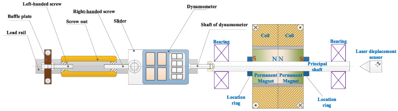
The aim of this design is to obtain greater negative stiffness that can be controlled conveniently. It is well known that the force between the PMs is stronger than the force between the current-carrying coils. Moreover, unlike the force between the PMs that cannot be controlled, the magnitude of the force between the current-carrying coils is controlled by the current. Furthermore, the shape of the magnet determines the distribution of the magnetic flux in the magnetic field, and the magnitude of the magnetic flux determines the magnitude of the magnetic force. Accordingly, to obtain greater force and controllability, a system consisted by PMs and the coils is designed in Fig. 1.

Fig. 1.

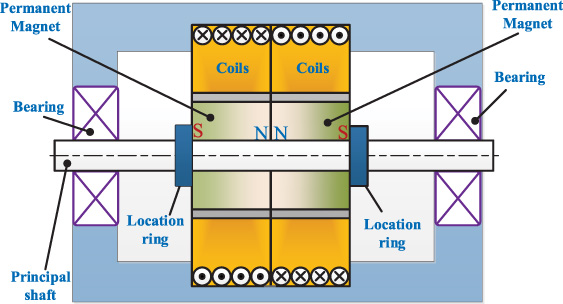
Schematic of the CENSS.

Figure 1 shows a schematic of the proposed CENSS. The CENSS consists of a principal shaft, two PMs, two identical circular copper coils, two location rings and two bearings. The two coils superposed by multiple solenoids fixed each other in position are coaxial and possess the same geometric dimension. The uniform distribution of current in the two coils is configured with the opposite direction. The coils become magnets when the current is switched on. Furthermore, the two PMs are fixed with respect to each other on the principal shaft by the two locating rings. The magnetization directions of PMs are opposite as shown in Fig. 1. Moreover, the principal shaft is supported by the two linear roll bearings at the ends of the shaft. The movement of the principal shaft with the two PMs is restricted along the axis direction of the two bearing holes. Then, in the expected initial position (where the coils coincide with the PMs), the shaft with PMs stay in a state of the equilibrium for the symmetry of the magnetic forces. But the equilibrium is extremely precarious. Once a small arbitrary perturbation acts on the shaft, the equilibrium will be broken and cannot be restored without additional force. Thus, the principal shaft exhibits a characteristic of negative stiffness which attributes to the magnetic force between the coils and PMs. The negative stiffness can be adjusted by changing the exciting current.

2. Calculation of the force and negative stiffness

This section presents the calculation of the magnetic force based on the filament method [15]. Based on the expression of the magnetic force and the relative displacement in the axial direction, the expression of stiffness of CENSS is deduced. The design parameters of the negative stiffness spring are shown in Table 1.

Table 1
Design parameters of the negative stiffness spring

Parameter Unit Definition

$R_a$ m Inner radius of the ring PM

$R_b$ m Outer radius of the ring PM

$R_c$ m Inner radius of the current-carrying coil

h m thickness of the coil

J T Polarization of the ring PM

a m Height of the ring PM

b m Height of the coil

c m the displacement of the center of the PMs to the center of the coils

μ₀ H⋅ m Magnetic constant (4π ×10⁷)

I A Excited current of the coils

Z_ij m The dispalcement from filament i to filament j

I_x m The current in the filament x

$R_x$ m The radius of filament x

U Half the number of the equivalent filaments of the PM

V Half the number of the axial of coils

W Half of the radial number of coils

Parameter	Unit	Definition
$R_a$	m	Inner radius of the ring PM
$R_b$	m	Outer radius of the ring PM
$R_c$	m	Inner radius of the current-carrying coil
h	m	thickness of the coil
J	T	Polarization of the ring PM
a	m	Height of the ring PM
b	m	Height of the coil
c	m	the displacement of the center of the PMs to the center of the coils
μ₀	H⋅ m	Magnetic constant (4π ×10⁷)
I	A	Excited current of the coils
Z_ij	m	The dispalcement from filament i to filament j
I_x	m	The current in the filament x
$R_x$	m	The radius of filament x
U		Half the number of the equivalent filaments of the PM
V		Half the number of the axial of coils
W		Half of the radial number of coils

2.1. Equivalence between permanent magnet and coils in the modeling

There are two common approaches to establish the model: the coulombian approach [16] and the amperian current approach [17]. Generally, the coulombian approach is chosen when the magnetism produced by a permanent magnet, while the amperian current approach is chosen when the magnetism produced by coils. For one system including PMs and the coils, it is important to choose which one in the two approaches.

Fig. 2.

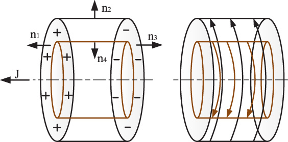
Equivalence between a ring permanent magnet and two solenoids.

A cylindrical permanent magnet and a solenoid own the same fictitious charge distribution [17]. On the basis of this concept and the principle of the magnetic field superposition, we propose a ring permanent magnet and two solenoids own the same fictitious charge distribution. Furthermore, compared the two approaches, the amperian current approach is adopted to establish the model. According to the amperian current approach, a three-dimensional schematic is shown in Fig. 2, which also illustrates the equivalence between a ring permanent magnet and two solenoids in this system. The equivalent current surface density of a permanent magnet is determined by the normal unit of the polarization, and satisfies as the following equation [17,18]: $\begin{eqnarray} \displaystyle \vec{k}={\displaystyle \frac{\vec{J}\times \vec{n}}{{\mu}_{0}}} & & \displaystyle \end{eqnarray}$ (1) Where $\vec{J}$ is the polarization of permanent magnet, $\vec{n}$ is the normal unit and μ₀ is the magnetic permeability in the air. In Fig. 2, the surfaces of the ring permanent magnet are composed of two cylinder and two tori. Then, according to the amperian current approach and ((1)), the equivalent current surface density on the ring permanent magnet can express by the following equations: $\begin{eqnarray}\displaystyle \text{} & \text{} & \displaystyle \vec{k_{1}}={\displaystyle \frac{\vec{J}\times \vec{n_{1}}}{{\mu}_{0}}}=0\end{eqnarray}$ (2) $\begin{eqnarray}\displaystyle \text{} & \text{} & \displaystyle \vec{k_{2}}={\displaystyle \frac{\vec{J}\times \vec{n_{2}}}{{\mu}_{0}}}={\displaystyle \frac{J}{{\mu}_{0}}}\vec{n_{2}}\end{eqnarray}$ (3) $\begin{eqnarray}\displaystyle \text{} & \text{} & \displaystyle \vec{k_{3}}={\displaystyle \frac{\vec{J}\times \vec{n_{3}}}{{\mu}_{0}}}=0\end{eqnarray}$ (4) $\begin{eqnarray}\displaystyle \text{} & \text{} & \displaystyle \vec{k_{4}}={\displaystyle \frac{\vec{J}\times \vec{n_{4}}}{{\mu}_{0}}}={\displaystyle \frac{J}{{\mu}_{0}}}\vec{n_{4}}.\end{eqnarray}$ (5) Because the phase difference between $\vec{n_{2}}$ and $\vec{n_{4}}$ is π, $\begin{eqnarray}\displaystyle \vec{k_{2}}=-\vec{k_{4}} & & \displaystyle\end{eqnarray}$ (6) Equation ((2)), ((4)) indicate that no equivalent current is existed on the two tori of the ring permanent magnet. And, ((3)), ((5)) show that the equivalent current surface density in the two cylinders hold the same volume and the opposite direction. Accordingly, it implies that a ring permanent magnet can be represented by two solenoids with the opposite current direction in the modeling.

Fig. 3.

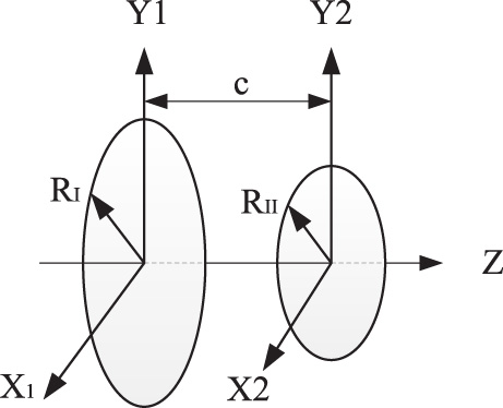
Helmholtz coils.

2.2. Calculation of the axial magnetic force and the stiffness

The filament method, whose reliability is proved in [15,19–22], is an effective approach in the magnetic force calculation. Modeling by the filament method, two identical current-carrying wires in the air are called Helmholtz coils [23], as shown in Fig. 3. The magnetic force between the wires is attractive under the same direction of the currents; conversely, the force is repulsive as the opposite direction of the currents. Due to calculating the magnitude of the scalar force between the wires, the analytic formulas can be expressed by: $\begin{eqnarray}\displaystyle \text{} & \text{} & \displaystyle F={\displaystyle \frac{{\mu}_{0}I_{1}I_{2}ck}{4\sqrt{R_{1}R_{2}}}}\left[{\displaystyle \frac{2-k^{2}}{1-k^{2}}}E(k)\right];\end{eqnarray}$ (7) $\begin{eqnarray} \displaystyle \text{} & \text{} & \displaystyle k^{2}={\displaystyle \frac{4R_{1}R_{2}}{(R_{1}^{2}+R_{2})^{2}+c^{2}}} \end{eqnarray}$ (8) Where R ₁ and R ₂ are the radiuses; I ₁ and I ₂ are the currents in the each wire; k is a transformer for the convenience in the expression.

K (k) is the complete elliptical integrals of the first kind: $\begin{eqnarray}\displaystyle K(k)=\int _{0}^{\frac{{\pi}}{2}}{\displaystyle \frac{1}{\sqrt{1-k\sin ^{2}{\theta}}}}d{\theta}. & & \displaystyle\end{eqnarray}$ (9)

E (k) is the complete elliptical integrals of the second kind: $\begin{eqnarray}\displaystyle E(k)=\int _{0}^{\frac{{\pi}}{2}}\sqrt{1-k\sin ^{2}{\theta}}d{\theta}. & & \displaystyle\end{eqnarray}$ (10)

Consider the two ring PMs and the two coils of this system subdivide in 2 × (2U +1) × (2V +1) + (2W +1) filaments, as shown in Fig. 4. U, V and W denote the number of the filaments of CENSS divided. The greater the values of U, V and W are, the more accurate the superposition calculation is. Furthermore, the magnetic force is related to the distance between the magnetic sources. The distance can be expressed by the displacement of the center of the PMs to the center of the coils, c. Moreover, each filament is acted on each other under the magnetic force. Thus, the calculation of the axial force exerted on PMs can be deduced by the superposition principle of the force between each filament.

Fig. 4.

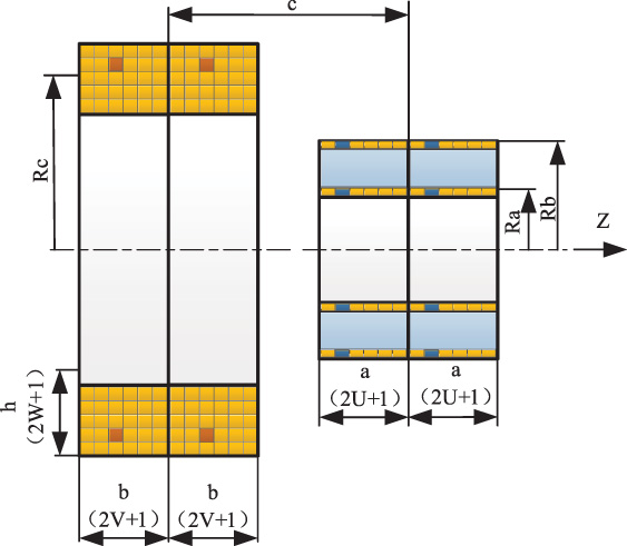
Meshes of the coils and PMs by the filament method.

Figure 4 shows that the coil is represented as a superposition of ring filaments, and the ring permanent magnet is represented as a superposition of solenoids. Inspired by the Helmholtz coils calculation, the filaments of the superposition calculation is configured, as shown in Fig. 5. It can be seen that six filaments are provided along the common axial direction, each filament of which represents the certain part of the CENSS shown in Fig. 4. The filament 1 and 4 represent the two coils fixed together. The filament 2 and 5 with the same diameter, represent the outer equivalent solenoids in the two PMs. The filament 3 and 6 with the same diameter, represent the inner equivalent solenoids in the two PMs. Thereby, for the two PMs held together, the displacement of the filaments 2, 3, 5 and 6 relate to the filaments 1 and 2, are the same. Moreover, I ₁ − I ₆ are the currents in the each filament. R ₁ − R ₆ are the radiuses in the each filament. Z _ij is the displacement between the filament i and the filament j. F _ij is the magnetic force between the filament i and the filament j. Furthermore, there are both attraction and repulsion in the configuration, for the direction of the current in the filament. And it is assumed that the direction Z is regarded as the positive direction.

Fig. 5.

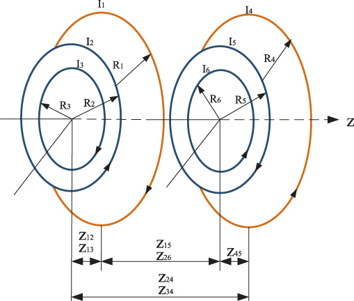
Unit of the superposition. The six circular current coils are in the air, which represent the unit of the equivalent current of the CENSS.

However, for the coils fixed together, the magnetic force between the filament 1and 4 formed by currents I ₁ and I ₄, F ₁₄ is ignored as the internal force. And F ₂₃, F ₂₅, F ₂₆, F ₃₅, F ₃₆, F ₅₆ are ignored as the internal force, for the same reason.

Thereby, according ((7)), ((8)) and the direction of the current, the unit of superposition of the magnecit force can be expressed by the following form: $\begin{eqnarray} \displaystyle \text{} & \text{} & \displaystyle F_{ij}=\mathrm{sig} n(e){\displaystyle \frac{{\mu}_{0}I_{i}I_{j}Z_{ij}k_{ij}}{4\sqrt{R_{i}R_{j}}}}\left[{\displaystyle \frac{2-k_{ij}^{2}}{1-k_{ij}^{2}}}E(k_{ij})-2K(k_{ij})\right] \end{eqnarray}$ (11) $\begin{eqnarray}\displaystyle \text{} & \text{} & \displaystyle k_{ij}^{2}={\displaystyle \frac{4R_{i}R_{j}}{(R_{i}+R_{j})^{2}+z_{ij}^{2}}}.\end{eqnarray}$ (12)

As shown in Fig. 4, for 2 × (2U +1) × (2V +1) + (2W +1) filaments, we can express the axial force exerted on PMs by the superposition of ((11)) as follows: $\begin{eqnarray}\displaystyle F={\displaystyle \frac{N_{1}N_{2}}{(2U+1)(2V+1)(2W+1)}}\mathop{\sum }_{i,j,g,s,l}F_{ij}(g,s,l) & & \displaystyle\end{eqnarray}$ (13) where $\begin{eqnarray} \displaystyle F_{ij}(g,s,l)\text{} & =\text{} & \displaystyle \text{sig}n(e)\frac{{\mu}_{0}I_{i}I_{j}Z_{ij}(g,s)k_{ij}(g,s,l)}{4\sqrt{R_{i}(l)R_{j}}}\nonumber\\ \displaystyle \text{} & \text{} & \displaystyle \quad \times \left[{\displaystyle \frac{2-k_{ij}^{2}(j,s,l)}{1-k_{ij}^{2}(j,s,l)}}E(k_{ij}(j,s,l))-2K(k_{ij}(j,s,l))\right]. \end{eqnarray}$ (14) $\begin{eqnarray}\displaystyle \text{} & \text{} & \displaystyle k_{ij}^{2}(j,s,l)={\displaystyle \frac{4R_{i}(l)R_{j}}{(R_{i}(l)+R_{j})^{2}+z_{ij}^{2}(g,s)}}\end{eqnarray}$ (15) $\begin{eqnarray}\displaystyle \text{} & \text{} & \displaystyle R_{i}(l)=R_{c}+{\displaystyle \frac{h}{2W+1}}l\end{eqnarray}$ (16) $\begin{eqnarray}\displaystyle \text{} & \text{} & \displaystyle R_{2}=R_{5}=R_{a};R_{3}=R_{6}=R_{b}\end{eqnarray}$ (17) $\begin{eqnarray}\displaystyle \text{} & \text{} & \displaystyle I_{j}={\displaystyle \frac{Ja}{N_{2}{\mu}_{0}}}l\end{eqnarray}$ (18) $\begin{eqnarray}\displaystyle \text{} & \text{} & \displaystyle Z_{12}(g,s)=Z_{13}(g,s)=Z_{45}(g,s)=Z_{46}(g,s)=c-{\displaystyle \frac{a}{2K+1}}g+{\displaystyle \frac{b}{2m+1}}s\end{eqnarray}$ (19) $\begin{eqnarray}\displaystyle \text{} & \text{} & \displaystyle Z_{15}(g,s)=Z_{16}(g,s)=c+{\displaystyle \frac{a+b}{2}}-{\displaystyle \frac{a}{2U+1}}g+{\displaystyle \frac{b}{2V+1}}s\end{eqnarray}$ (20) $\begin{eqnarray}\displaystyle \text{} & \text{} & \displaystyle Z_{42}(g,s)=Z_{43}(g,s)={\displaystyle \frac{a+b}{2}}-c+{\displaystyle \frac{a}{2U+1}}g-{\displaystyle \frac{b}{2V+1}}s\end{eqnarray}$ (21) $\begin{eqnarray}\displaystyle \text{} & \text{} & \displaystyle e=\left\{\begin{array}{@{}ll@{}}1, & \text{for }ij=12,16,45,42\\ -1, & \text{for }ij=13,15,46,43\end{array}\right.\end{eqnarray}$ (22) $\begin{eqnarray}\displaystyle \text{} & \text{} & \displaystyle i=\{1,4\}\end{eqnarray}$ (23) $\begin{eqnarray}\displaystyle \text{} & \text{} & \displaystyle j=\{2,3,5,6\}\end{eqnarray}$ (24) $\begin{eqnarray}\displaystyle \text{} & \text{} & \displaystyle g=\{-U\ldots 0\ldots U\}\end{eqnarray}$ (25) $\begin{eqnarray}\displaystyle \text{} & \text{} & \displaystyle s=\{-V\ldots 0\ldots V\}\end{eqnarray}$ (26) $\begin{eqnarray}\displaystyle \text{} & \text{} & \displaystyle l=\{-W\ldots 0\ldots W\}.\end{eqnarray}$ (27) N ₁ is the turns of the coils. N ₂ is the turns of equivalent currents of the PMs.

Based on (13), the axial stiffness of the CENSS is the derivative of the force with respect to the relative axial displacement c as follow: $\begin{eqnarray}\displaystyle K(c)=-{\displaystyle \frac{dF}{dc}}. & & \displaystyle\end{eqnarray}$ (28)

3. Parametric study and analysis of the modeling

According to (14), it is observed that both currents in the coils, I _i, and the equivalent current of the PMs, I _j, have the same effect on the force and stiffness. And the equivalent current I _j is governed by the polarization of the PMs, which is irrevocable from being produced. However, the I _i can be easy controlled by using the current controller. Thereby, adjusting to the force and stiffness can be obtained by the change of current in the coils I _i.

From (13), it is observed that the turns of coils N ₁ and the turns of equivalent currents N ₂ bear on the force and stiffness. Furthermore, the change of N ₁ is obtained by the way of making the coils, and change of N ₂ is obtained using changing the thickness of the PMs. Moreover, the change of N ₁ and N ₂ lead to the change of dimensions of the coils and PMs respectively. Thus, the influence of N ₁ and N ₂ transform to the dimension’s optimization of coils and PMs.

It is well known that the bigger the dimensions of the PMs are, the greater the magnetic force is. But in the actual work, it is hard to unlimited change the radius of the PMs and the coils in order to enhance the magnet force. Meanwhile, the current of the coils cannot increase infinitely for the characteristic of the material. Thus, in order to obtain the greater force, it is necessary that the dimensions of the coils and PMs are optimized.

The smaller air gap is, the greater an axial force is [9]. But for the necessary of non-touching in the actual working, the set of the gap is 0.00075 m between the PMs and the coils. Moreover, in order to obtain greater current in the coils, 0.0005 m is adopted as the diameter of copper wire. Lastly, it takes J = 1.19 T for adopting the NDFeB35 (1.17 T–1.21 T).

3.1. Influence of turns of the coils on the axial magnetic force and the stiffness

When the parameters of the PMs as constant are assumed, the representation of the axial magnetic force and stiffness relate to the turns of coils are studied. Basically, with the increase of turns of the coils in constant radius, the thickness of the coils is increased. Then, for the convenience expression, the equivalent thickness of the coil is used to represent the turns of the coils, whose 0.001 m thick stands for 30 turns.

Fig. 6.

The axial magnetic force F versus the equivalent thickness of the coils and the displacement c. Calculation by ((13)) with the following parameters: R _a = 0.005 m, R _b = 0.015 m, h = 0.00925 m, a = 0.01 m, R _c = 0.020375 m, J = 1.19 T, I _i = 0.7 A.

Fig. 7.

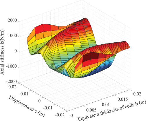
The axial stiffness k versus the equivalent thickness of the coils and the displacement c. Calculation by ((28)) with the following parameters: R _a = 0.005 m, R _b = 0.015 m, h = 0.00925 m, a = 0.01 m, R _c = 0.020375 m, J = 1.19 T, I _i = 0.7 A.

Figure 6 and Fig. 7 represent the relationship between the equivalent thickness of the coils and the magnetics force and the stiffness, respectively. The greater the equivalent thickness of the coils, the greater the value of magnetic force and stiffness. And, as shown in Fig. 7, it is clear that the stiffness of the CENSS is negative as the displacement is in a certain range. The maximum value of negative stiffness appears at the position where the displacement is zero, and, the position does not change with the equivalent thickness of the coils. The increment of magnetic force and stiffness is nonlinear with the increment of the equivalent thickness of the coil.

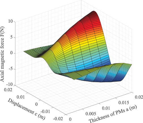
3.2. Influence of the PMs thickness on the axial magnetic force and the stiffness

Fig. 8.

The axial magnetic force F versus the thickness of PMs and the displacement c. Calculation by ((13)) with the following parameters: I _i = 0.7 A, R _a = 0.005 m, R _b = 0.015 m, h = 0.00925 m, b = 0.01 m, R _c = 0.020375 m.

Fig. 9.

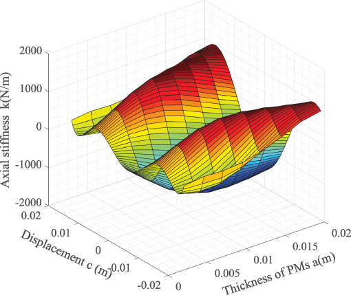
Representation of axial stiffness k versus the thickness of PMs and the displacement c. Calculation by ((28)) with the following parameters: I _i = 0.7 A, R _a = 0.005 m, R _b = 0.015 m, h = 0.00925 m, b = 0.01 m, R _c = 0.020375 m.

Other parameters are fixed, and the thickness of the PMs is a variable. Figures 8 and 9 represent the relationship between the thickness of the PMs and the magnetic force and the stiffness, respectively. Similar to the effect of the equivalent thickness of the coils on the magnetic force and the stiffness, The greater the thickness of the PMs, the greater the value of magnetic force and stiffness. As shown in Fig. 9, it is clear that the stiffness of the CENSS is negative as the displacement is in a certain range.The maximum value of negative stiffness appears at the position where the displacement is zero, and, the position does not change with the thickness of the PMs. The increment of magnetic force and stiffness is nonlinear with the increment of the thickness of the PMs.

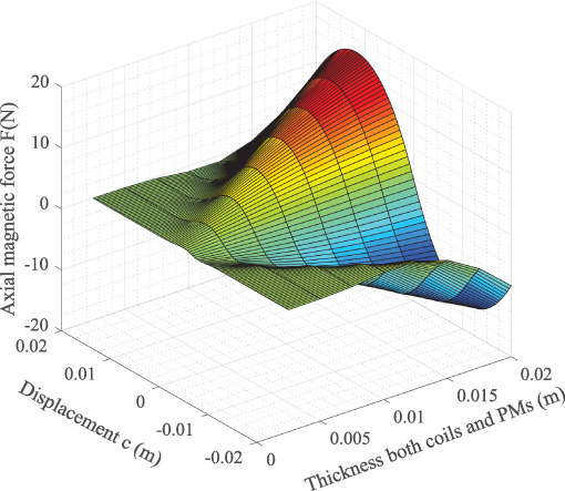
3.3. Influence of the same thickness of the PMs and the coils on the axial magnetic force and the stiffness

Fig. 10.

The axial magnetic force F versus the same thickness of the PMs and the coils and the displacement c. Calculation by ((13)) with the following parameters: I _i = 0.7 A, R _a = 0.005 m, R _b = 0.015 m, h = 0.00925 m, a = b = 0.01 m, R _c = 0.020375 m.

Fig. 11.

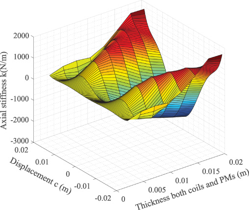
The axial stiffness of the magnetic force F versus the same thickness of the PMs and the coils and the displacement c. Calculation by ((28)) with the following parameters: I _i = 0.7 A, R _a = 0.005 m, R _b = 0.015 m, h = 0.00925 m, a = b = 0.01 m, R _c = 0.020375 m.

The influence of the same thickness change of the PMs and the coils on the magnetic force and stiffness are shown in Fig. 10 and Fig. 11. It is shown that the greater the thickness is, the greater the magnetic force and the negative stiffness are. But it is observed that the axial magnetic force and stiffness are increased in equal-ratio with the thickness increasing. And, both the range and amplitude of the negative stiffness become larger, as the thickness increasing.

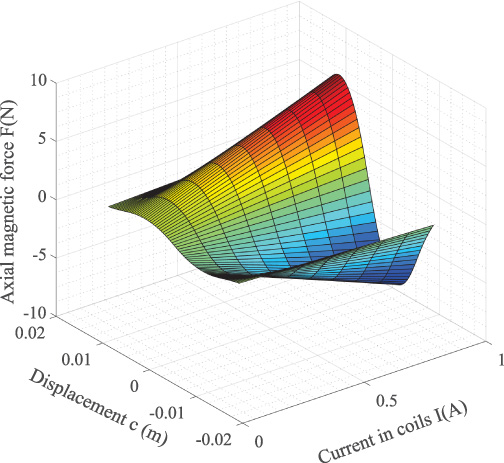
3.4. Influence of the current in the coils on the axial magnetic force and the stiffness

Fig. 12.

The axial magnetic force F versus displacement c and the currents in coils I. Calculation by ((12)) with the following parameters: R _a = 0.005 m, R _b = 0.015 m, h = 0.00925 m, a = b = 0.01 m, R _c = 0.020375 m, J = 1.9 T.

Fig. 13.

The axial stiffness of the magnetic force F versus the current in the coils and different displacement c. Calculation by ((28)) with the following parameters: R _a = 0.005 m, R _b = 0.015 m, h = 0.00925 m, a = b = 0.01 m, R _c = 0.020375 m, J = 1.9 T.

Figure 12 and Fig. 13 show that the influence of the current on the axial magnetic force and stiffness, respectively. It can be seen that a nonlinear relationship is existed between the displacement and the magnetic force and stiffness. And the stiffness is negative in a certain range of displacement, which is expected in the vibration isolation field. Furthermore, from Fig. 13, the stiffness is symmetrical relate to the axial of the zero displacement, which is obtained the negative maximum at zero displacement. Meanwhile, the greater the current is, the greater the axial magnetic force and stiffness is. Moreover, the change of the stiffness is linearly related to the current. However, regardless of how the current changes, it is a fixed constant that the range of the negative stiffness in the displacement. As a result, on-line control of the force and the stiffness can be achieved by changing the current, keeping the range of negative stiffness in the displacement.

3.5. Discussion of the parameters

From the above parameter study, it can be found that the change of the equivalent thickness of the coil and the thickness of the permanent magnet can make the stiffness change. Comparing Fig. 7 and Fig. 9, it can be found that the change in the thickness of the PMs has a greater impact on the stiffness than the change in the equivalent thickness of the coil. If the equivalent thickness of the coil and the thickness of the permanent magnet are the same change, a larger adjustment range of stiffness can be obtained from 11. Although the thickness can change the stiffness, the physical structure of the system needs to be changed, and online adjustment cannot be achieved.

From Fig. 13, it can be found that the current in the coils can adjust the stiffness, and the change of the current has a linear relationship to the change of the stiffness. Compared using the method of changing the thickness of the coils and the PMs to change the stiffness, the method of changing the current can realize the online adjustment of the stiffness. Due to the linear relationship and the easy controllability of the current, the method of the online adjustment of stiffness becomes convenient by the method of changing the current.

4. Experimental study

4.1. Set-up of the experiment

In order to measure the stiffness of the CENSS, both the axial magnetic force and displacement in the principal shaft are confirmed necessarily. The apparatus of testing the force and displacement is designed, as shown in Fig. 14. The principal shaft and the shaft of dynamometer are in threaded connection, and the dynamometer is fixed on the slider. Therefore, there is the same displacement among the slider, the dynamometer and the principal shaft. Moreover, the displacement can be generated by rotating the screw nut. Thereby, the precise magnitude of the displacement is obtained from the laser displacement sensor and the axial magnetic force reads from the dynamometer. In addition, the changes in current are achieved by a current driver.

Fig. 14.

Schematic of experimental set-up.

A laboratory scale apparatus was built in lab. Figure 15 shows a photo of the experimental setup. In order to isolate the interference from ground vibration, the apparatus was installed on a pneumatic platform. The displacement between the coils and the PMs was adjusted 2 mm by rotating the screw nut one turn, because of the thread pitch of the screws is 1 mm. The precise displacement was measured by a KEYENCE LK-G30A type CCD laser displacement sensor for the kinematic errors in the screw nut rotating. The axial magnetic force was measured by an ELECALL ELK-10 type digital force gauge. The currents in the coils were controlled by the system which consists of PXI platform (NI PXI-1024Q), analog output module (NI-PXI6733) and current driver (Accelnet Micro Panel ACJ-055-18).

Fig. 15.

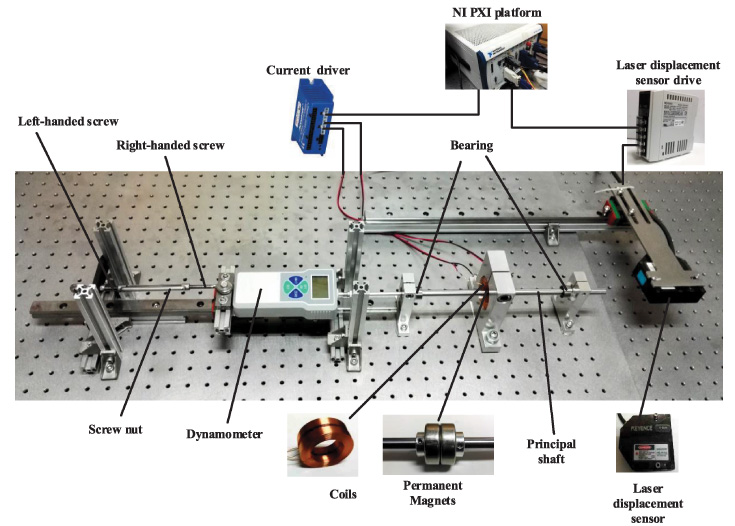
Photo of the experimental setup.

The displacement is observed from the CCD laser displacement sensor which can distinguish 0.0001 mm, and the force is read from the dynamometer which can distinguish 0.01 N. Moreover, the current in the coils is controlled by the NI PXI system. Finally, the result obtained from the experiments contrast to the calculation.

The experimental procedure is designed. First, test the equilibrium position of the coils and the PMs. Rotate the screw nut and observe the reading of the dynamometer. When the dynamometer shows zero, the axial position of the coils and the PMs coincide. Second, test the position where the magnetic force on the left side of the equilibrium positioned is zero. Adjust the screw nut, observe the laser displacement sensor, and move the permanent magnet 0.015 m to the left. Finally, the magnetic force is measured at an axial interval of 0.0005 m. Adjust the screw nut, observe through the laser displacement sensor every 0.0005 m of movement, and record the measured force count value. The test is completed until the position where the magnetic force on the right side of the equilibrium is zero is found.

4.2. Experimental results

Fig. 16.

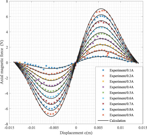
Comparisons of the experiment and the calculation in the axial magnetic force F relate to displacement c. R _a = 0.005 m, R _b = 0.015 m, h = 0.00925 m, a = 0.009 m, b = 0.009 m, N ₁ = 306, R _c = 0.020375 m, J = 1.19 T.

The force comparisons between calculative results and experiments are shown in Fig. 16. The calculative results are calculated by ((13)). It is observed that there is a good agreement to the calculated results and experimental measurement. The nonlinearity is exhibited in the axial magnetic force F respect to the displacement c. The closer the zero displacement is, the closer the force is to the experimental and calculated results. And the smaller the current in the coils is, the smaller the error of the force is to the experimental and calculated results.

Fig. 17.

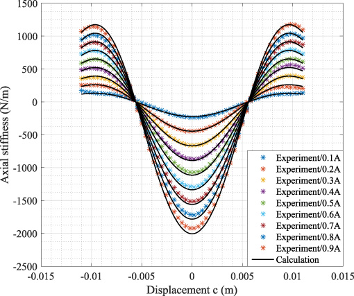
Comparisons of the experiment and the calculation in the axial stiffness k relate to the displacement c. R _a = 0.005 m, R _b = 0.015 m, h = 0.00925 m, a = 0.009 m, b = 0.009 m, N ₁ = 306, R _c = 0.020375 m, J = 1.19 T.

From the expression of the stiffness of the reference spring by (28), the stiffness comparisons between calculated and experimental results are shown in Fig. 17. It can be seen that there is a certain region in which the stiffness is always negative in the displacement c. And the maximum of the negative stiffness is obtained at the zero displacement, which is desired in the vibration isolation. The change in the stiffness from 237 N/m to 1920 N/m can be achieved by changing the current. Furthermore, the volume of the maximum is governed by the currents in the coils. The smaller the current in the coils is, the more similar the stiffness is to result from the experiment and the calculation. Then, at the every displacement, the stiffness curves are equidistantly distributed.

Fig. 18.

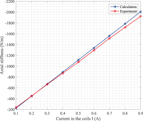
Comparisons between the axial stiffness experiment and the calculation at equilibrium position (zero displacement). R _a = 0.005 m, R _b = 0.015 m, h = 0.00925 m, a = 0.009 m, b = 0.009 m, N ₁ = 306, R _c = 0.020375 m, J = 1.9 T.

The performance of the NSS at the equilibrium position is the focus of the study. The performance of CENSS at the equilibrium position is shown on Fig. 18. The greater the current in the coils is, the greater the negative stiffness is. It is observed that there is a liner relationship between current in the coils and the axial stiffness. In addition, the error between the calculation and the experiment increases with increasing of the current in the coils, which it’s maximum cannot up to 2%.

Fig. 19.

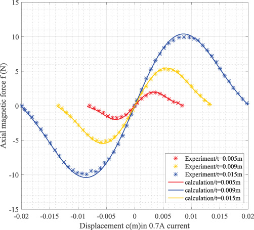
Comparisons the axial forces between the experiment and the calculation in different thickness. (t stand for the same thickness of PMs and coils).

Fig. 20.

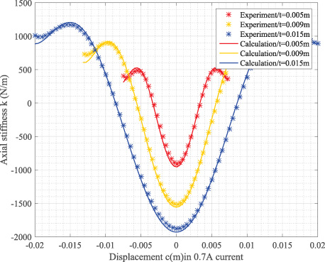
Comparisons the axial stiffness between the experiment and the calculation in different thickness. (t stand for the same thickness of PMs and coils.)

The axial magnetic force and the stiffness of CENSS in different thicknesses are shown in Fig. 19 and Fig. 20. It is observed that the different thickness in CENSS possess similar curves distribution about the force and the stiffness. From Fig. 20, the change of thickness affects not only the range of negative stiffness in displacement but also the maximum value of negative stiffness.

From the results shown from Fig. 16 to Fig. 20, there are three key points. Firstly, keeping a constant in the range of negative stiffness, the magnitude of the negative stiffness can be controlled by changing the current of the coils. And, at zero displacement, the extremum of the negative stiffness of the CENSS is linearly related to the current in the coils. Secondly, the different thickness in CENSS can produce the different negative stiffness. At last, the calculated results show a good agreement with the experimental results.

5. Discussion

The calculation of CENSS is proved by the experiments. The designed spring can provide the nonlinear negative stiffness to the vibration isolation. The maximum of the negative stiffness is appeared at equilibrium position, which will bring a lot of advantages to vibration isolation. Firstly, at equilibrium position QZS will be obtained from the CENSS by parallel connection with a positive stiffness spring. As a result, it can promote the efficiency of the isolator with the CENSS in the low frequency vibration. Secondly, for the nonlinear characteristic of the magnetic negative stiffness, in the away direction of the equilibrium position the stiffness of the spring can increase from negative to positive. Therefore, the dynamic and static performances of the isolator with the CENSS are improved. Finally, the stiffness can be controlled by adjusting the current in the coils, which can make the isolator to adapt to dynamic varied load at the working.

From the analysis of the CENSS in Section 3 and Section 4, the CENSS can realize varied negative stiffness if the current in the coils is not a fixed constant. And the nonlinear behavior of the negative stiffness can be controlled by the current in the coils. This means that the CENSS can be used more widely.

6. Conclusions

This paper presents a controllable negative stiffness spring which consists of the PMs and the current coils. The calculated expression of the axial magnetic force and the stiffness are derived and validated by the experiments. The following conclusion can be drawn:

(1) The stiffness of the CENSS can be controlled by the change of the current in the coils, which is a non-linear negative stiffness. And the maximum negative stiffness is obtained at equilibrium position.

(2) The negative stiffness at equilibrium position is linear correlate to the volume of the current. And the control of the stiffness is achieved by changing the current in the coils.

(3) If the thickness of PMs equals to equivalent thickness of the coils, the CENSS can produce the max controlled negative stiffness.

In the future work, we plan to research the method of control about the CENSS to achieve a perfect active VIS and test the performance in VIS.

References

Carrella

Brennan

M.J.

and Waters

T.P.

, Static analysis of a passive vibration isolator with quasi-zero-stiffness characteristic, J. Sound Vib. 301(3-5) (2007), 678–689.

Kovacic

Brennan

M.J.

and Waters

T.P.

, A study of a nonlinear vibration isolator with a quasi-zero stiffness characteristic, J. Sound Vib. 315(3) (2008), 700–711.

Karthick

Saran Kumar

and Mohan

, Relative analysis of controller effectiveness for vertical plane control of an autonomous underwater vehicle, in: OCEANS 2016-Shanghai, IEEE, 2016, pp. 1–6.

Lan

C.C.

Yang

S.A.

and Wu

Y.S.

, A Design and experiment of a compact quasi-zero-stiffness isolator capable of a wide range of loads, J. Sound Vib. 333(20) (2014), 4843–4858.

Antoniadis

Chronopoulos

Spitas

, Hyper-damping properties of a stiff and stable linear oscillator with a negative stiffness element, J. Sound Vib. 346 (2015), 37–52.

T.D.

Bui

M.T.N.

and Ahn

K.K.

, Improvement of vibration isolation performance of isolation system using negative stiffness structure, IEEE/ASME Trans. Mech. 21(3) (2016), 1561–1571.

T.D.

Bui

M.T.N.

and Ahn

K.K.

, Vibration isolation characteristics of a nonlinear isolator using Euler buckled beam as negative stiffness corrector: A theoretical and experimental study, J. Sound Vib. 333(4) (2014), 1132–1148.

Zhou

Wang

, Nonlinear dynamic characteristics of a quasi-zero stiffness vibration isolator with cam-roller-spring mechanisms, J. Sound Vib. 346 (2015), 53–69.

Zhu

, Modeling of axial magnetic force and stiffness of ring-shaped permanent-magnet passive vibration isolator and its vibration isolating experiment, IEEE Trans. Magn. 48(7) (2012), 2228–2238.

10.

Zhang

Kou

Jinu

, Research on a low stiffness passive magnetic levitation gravity compensation system with opposite stiffness cancellation, IEEE Trans. Magn. 50(11) (2014), 1–4.

11.

Chen

and Shan

, Analysis and experiment of a vibration isolator using a novel magnetic spring with negative stiffness, J. Sound Vib. 333(13) (2014), 2958–2970.

12.

Shi

and Zhu

, Magnetic negative stiffness dampers, Smart Mater. Struct. 24(7) (2015), 072002.

13.

Hyun

M.W.

Yoo

Hwang

S.T.

, Optimal design of a variable stiffness joint using permanent magnets, IEEE Trans. Magn. 43(6) (2007), 2710–2712.

14.

Anubi

O.M.

and Crane

, A new semiactive variable stiffness suspension system using combined skyhook and nonlinear energy sink-based controllers, IEEE Trans. Control Syst. Technol. 23(3) (2015), 937–947.

15.

Babic

and Akyel

, New formulas for mutual inductance and axial magnetic force between magnetically coupled coils: Thick circular coil of the rectangular cross-section-thin disk coil (Pancake), IEEE Trans. Magn. 49(2) (2013), 860–868.

16.

Ravaud

Lemarquand

and Lemarquand

, Force and stiffness of passive magnetic bearings using permanent magnets. Part 1: Radial magnetization, IEEE Trans. Magn. 45(7) (2009), 2996–3002.

17.

Ravaud

Lemarquand

Babic

, Cylindrical magnets and coils: Fields, forces, and inductances, IEEE Trans. Magn. 46(9) (2010), 3585–3590.

18.

Robertson

Cazzolato

and Zander

, A simplified force equation for coaxial cylindrical magnets and thin coils, IEEE Trans. Magn. 47(8) (2011), 2045–2049.

19.

Wang

Z.J.

and Ren

, Magnetic force and torque calculation between circular coils with nonparallel axes, IEEE Trans. Appl. Supercond. 24(4) (2014), 1–5.

20.

Babic

Sirois

Akyel

, New formulas for mutual inductance and axial magnetic force between a thin wall solenoid and a thick circular coil of rectangular cross-section, IEEE Trans. Magn. 47(8) (2011), 2034–2044.

21.

Babic

and Akyel

, Magnetic force calculation between thin coaxial circular coils in air, IEEE Trans. Magn. 44(4) (2008), 445–452.

22.

Kim

K.B.

Levi

Zabar

, Mutual inductance of noncoaxial circular coils with constant current density, IEEE Trans. Magn. 33(5) (1997), 4303–4309.

23.

Trout

S.R.

, Use of Helmholtz coils for magnetic measurements, IEEE Trans. Magn. 24(4) (1988), 2108–2111.