An omnidirectional WPT platform for distributed fully implanted neural recording systems

Abstract

Recent progress on human brain science requires developing advanced neural recording system to capture the activity of large neural populations accurately, across a large area of the brain, and over extended periods. Recently proposed distributed neural recording systems with numerous implanted devices require reliably energizing them wirelessly. Random distribution of these mm-sized implants and brain motion place them at different positions and orientations with respect to the power transmitter. Therefore, traditional wireless power transfer techniques fall short of reaching sufficient power for all implants simultaneously, rendering some implants nonfunctional. In this paper, a three-layer power transmitting array with three-phase coil excitation current is introduced, which is capable of producing omnidirectional and homogeneous magnetic field across the volume where the Rx coils are located. The individual coil dimensions in the array is optimized to improve the worst-case scenario in terms of homogeneity, which is further verified by the measurements using a scaled-up prototype system. The measurement results show that the minimum received voltages is improved from 0.34 V for 10-mm side-length hexagonal transmitting coil array to 0.83 V for the optimal case, i.e., 35 mm side-length hexagonal transmitting coil array.

Keywords

Omnidirectional distributed wireless power transfer three-phase three-layer coil array coil radius optimization

1. Introduction

With societies aging, considerable attention is being paid to healthcare. The human brain with ∼85 billion neurons and 100 trillion synapses is the most complicated organ in the body. The diseases that involve the brain are usually severe and long-term, resulting in loss of function, considerable costs, and reduced quality of life. If the commands initiated in the brain cannot reach other organs, such as limbs, because of a damage in the path of the neural signal transmission, the result will be paralysis. Brain-machine interfacing (BMI) is a promising technology to realize “actions from thoughts” [1] by recording and analyzing the neural signal to detect the user intentions, and then generating appropriate signals for stimulating the neural prostheses or controlling mechanical devices like robotic arms. A pioneering example is shown in [2], in which scientists used a BMI to help a patient control a robotic arm to drink from a cup, all by herself. In this system, a 96-channel microelectrode array was implanted in the motor cortex of a paralyzed patient, and the signals were delivered by wires. For long term use, however, the hardwired implanted devices, which are anchored to the skull, can lead to inflammation, cell death, and damage to the blood brain barrier due to brain micromotions, which are not safe enough for routine clinical applications [3]. Besides the longevity problem, the traditional neural recording method by implanting a centralized array in the cortex cannot cover enough area of the brain, which is a requirement for a viable BMI because different clusters of neurons at different locations act together for more complex functions and require the implants to record their activities at those positions simultaneously [4].

In the face of these challenges, distributed neural recording system with small implantable microelectronic devices (IMDs) over the target brain surface are proposed to replace the traditional single centralized IMD [5–7]. In order to eliminate the tethering effect of the power and signal transfer wire, not only signal but also power should be transferred wirelessly. Wireless power transfer (WPT) is a feasible technique to energize the IMDs wirelessly which has also been used in many other areas such as consumer electronics [8], electronic vehicles [9], and biomedical devices [10]. Although some researchers realized WPT for small IMDs via ultrasound [11] or laser [12] coupling, the WPT to IMD is often established via electromagnetic (EM) field coupling [13].

In neural recording application, however, at least 2 challenges still exist to realize an effective WPT system. Firstly, the size of the implants are very small in the order of a millimeter to minimize damage to the surrounding tissue [14]. The power transfer efficiency (PTE) decreases with dimensions of the receiver (Rx) coils for a fixed power transfer distance, which will result in delivering insufficient power to the load (PDL) when staying within safe limits of human body exposure to EM field. A key indicator of the tissue EM exposure is the specific absorption rate (SAR), which should not exceed 1.6 W/kg according to the IEEE standard [15]. The SAR is determined by the electric field intensity induced in tissue which limits the transmitter (Tx) power that can be applied. Generally, high PTE is required to ensure sufficient PDL without the risk of overheating the tissue.

Secondly, the implants is randomly distributed over a large area. In order to cover a large area, one solution is using far-field EM radiation using omnidirectional antennas [16]. The drawback of far-field EM radiation is low PTE. Because the power is lost in the volume where there is no IMDs. The near-field inductively-coupled WPT, which usually works at resonance to improve the PTE and transfer distance, is studied comprehensively following the work by a group from MIT [17]. The schematic of a two-coil inductively-coupled near-field WPT is shown in Fig. 1, where V _S and R _L are the equivalent power source and load, respectively. The coupling between Tx and Rx coils can be expressed in terms of their coupling coefficient (k) or mutual inductance (M), which are related as k = M∕(L ₁ L ₂)^0.5, where L ₁ and L ₂ are the self-inductances of the Tx and Rx coils, respectively. The maximum achievable PTE, 𝜂_M, is reached by inserting impedance compensation circuits in the Tx and Rx sides [18], $\begin{eqnarray}\displaystyle {\eta}_{M}={\displaystyle \frac{k^{2}Q_{1}Q_{2}}{\left(1+\sqrt{1+k^{2}Q_{1}Q_{2}}\right)^{2}}}, & & \displaystyle\end{eqnarray}$ (1) where Q ₁ and Q ₂ are the quality factors of the Tx coil and Rx coil, respectively. We can observe from (1) that the product of the quality factors and the square of coupling coefficient are critical parameters. Optimizing geometries of the coils to improve the quality factor is one way to improve the PTE. Other than quality factors, which are only the function of geometries, like the number of turns, width of the wire, space between adjacent wires, etc., the coupling coefficient is a function of the relative position and angle between the Tx and Rx coils [19]. In the application of distributed fully implanted devices, the implants are positioned at different locations of interest on the surface of the brain. The brain topography with sulci and gyri leads to the orientations of the Rx coils being uncertain. If the orientation of one Rx coil is perpendicular to the orientation of the Tx coil, the magnetic field (H-field) produced by the Tx coil will not pass through it and no power will be transferred. This angular results in “dead spots”. At the same time, in order to cover all the Rx coils, the size of the Tx coil should be large enough. The scheme of a large Tx coil and a small Rx coil link results in low coupling coefficient and low PTE [20].

Unlike the traditional WPT system design, in which the system is usually optimized for the best case scenario with Tx and Rx coils coaxially oriented to keep all the implants being energized in the neural recording system, the worst case should be considered to satisfy the power requirement. From the system optimization point of view, a Tx which can produce an omnidirectional and homogeneous H-field is required.

Fig. 1.

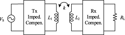
A diagram of a two-coil inductively-coupled WPT system.

Fig. 2.

Rendering of a distributed neural recording system with fully implanted sensors, which are wirelessly powered by a planar array of external Tx coils [7].

In this paper a three-layer power transmitting array with three-phase coil excitation current is designed and optimized for potential application in distributed neural recording with fully implanted sensors, as shown in Fig. 2. Prior work on the Tx array is reviewed in Section 2. The basic principle of optimizing the Tx array is calculating the H-field produced by all the coil array, which is discussed in Section 3 followed by optimizing the Tx coil array geometry in Section 4. The experimental results of the prototype WPT platform is shown in Section 5, followed by the discussion and conclusions in Sections 6 and 7, respectively.

2. Related works

Efforts have been made to resolve the dead-spot problem and improve the PTE. It has been established that a Tx array comprised of many coils can extend the coverage area [21,22]. According to the phase difference between the excitation currents of two adjacent coils, arrays have types of in-phase [23,24], out-of-phase [25,26], and three-phase [27,28], as shown in Figs 3a, 3b and 3c respectively, where hexagonal-shaped coils are used. In in-phase and out-of-phase types, some or all adjacent sides of the neighboring coils have opposite current directions, which cancel out each other in these sides. Although square-shaped coil arrays with out-of-phase excitation current [29] can avoid the current cancellation of adjacent sides, the H-field in the vertical direction upon these sides will be canceled, as pointed out in [28]. The three-phase type is a trade-off between in-phase and out-of-phase types, and makes the H-field more homogeneous.

Fig. 3.

Three types of Tx array: (a) in-phase, (b) out-of-phase, and (c) three-phase.

Fig. 4.

Schematic of the three-layer array.

The three-phase excitation can be considered as averaging the phase of the excitation currents. In order to make the distribution of the H-field even more homogeneous, three layers of three-phase excitation can be assembled with a staggered form, as shown in Fig. 4 [30], where each layer, designated with a different color, is activated with 1/3rd duty cycle. In other words, the coil layers are time division multiplexed, which averages the H-field produced by each layer. In fact, if the array is one-layer type and all the cells work at the same time, dead spots will still exist. Three-layer type is proven to be a feasible approach to cancel the dead spots [30]. In Sections 3 and 4, this three-layer three-phase array is optimized by sweeping the unit coil geometry.

3. Magnetic field distribution

Finding the current source distribution from the known distribution of H-field is an inverse problem whose solution is often not easy and does not exist explicitly. Instead, numerical methods, finite element analysis (FEM), and parameter sweeps are used to optimize the coil geometry in the Tx array, which will be done after calculating the H-field distribution of the Tx array.

The H-field distribution is the vector sum of the H-fields produced by all the hexagonal coils in one layer which are active at the same time. The accurate H-field produced by a hexagonal coil can be calculated by decomposing the coil into six separate straight filaments and then summing up the H-field of each filament. The H-field at an arbitrary point P produced by the ith circular coil with excitation current proportional to cos(ωt + θ_i), as shown in Fig. 5a, can be found in [31]. For example, the H-field produced by the side p _1i p _2i is $\begin{eqnarray}\displaystyle H_{p_{1i}p_{2i}}\text{} & =\text{} & \displaystyle {\displaystyle \frac{1}{4{\rm\pi}\sqrt{\left(\sqrt{3}a_{i}-y\right)^{2}+z^{2}}}}\nonumber\\ \displaystyle \text{} & \text{} & \displaystyle \quad \times ∼\left({\displaystyle \frac{a_{i}+x}{\sqrt{\left(\sqrt{3}a_{i}-y\right)^{2}+z^{2}+(a_{i}+x)^{2}}}}+{\displaystyle \frac{a_{i}-x}{\sqrt{\left(\sqrt{3}a_{i}-y\right)^{2}+z^{2}+(a_{i}-x)^{2}}}}\right),\end{eqnarray}$ (2) where the sides of the coil are denoted as a _i. To simplify the math and without loss of generality, the hexagonal coils are approximated by circular coils with the same diameter, as shown in Fig. 5b, where the H-field at an arbitrary point P produced by the ith circular coil can be found in [32]. The H-field can be divided into the x-, y-, and z-components in the Cartesian coordinate system, i.e., H _xi = A _xi cos(ωt + θ_i), H _yi = A _yi cos(ωt + θ_i), and H _zi = A _zi cos(ωt + θ_i), respectively. The amplitudes A _xi, A _yi, and A _zi are given by, $\begin{eqnarray}\displaystyle \begin{array}{@{}l@{}}\displaystyle A_{xi}={\displaystyle \frac{z}{4{\rm\pi}{\rho}_{i}}}\sqrt{{\displaystyle \frac{m_{i}}{a_{i}{\rho}_{i}}}}\left({\displaystyle \frac{2-m_{i}}{2-2m_{i}}}E(m_{i})-K(m_{i})\right)\cos ({\varphi}_{i})\\[16.0pt] \displaystyle A_{yi}={\displaystyle \frac{z}{4{\rm\pi}{\rho}_{i}}}\sqrt{{\displaystyle \frac{m_{i}}{a_{i}{\rho}_{i}}}}\left({\displaystyle \frac{2-m_{i}}{2-2m_{i}}}E(m_{i})-K(m_{i})\right)\sin ({\varphi}_{i})\\[16.0pt] \displaystyle A_{zi}={\displaystyle \frac{1}{4{\rm\pi}{\rho}_{i}}}\sqrt{{\displaystyle \frac{m_{i}}{a_{i}{\rho}_{i}}}}\left({\displaystyle \frac{a_{i}m_{i}-(2-m_{i}){\rho}_{i}}{2-2m_{i}}}E(m_{i})+{\rho}_{i}K(m_{i})\right)\\[16.0pt] \displaystyle m_{i}={\displaystyle \frac{4a_{i}{\rho}_{i}}{((a_{i}+{\rho}_{i})^{2}+z^{2})}},\end{array} & & \displaystyle\end{eqnarray}$ (3) where 𝜌_i, φ_i, and z are the radial distance, azimuth angle, and height, respectively, in the cylindrical coordinate system supposing that the cen ter of the ith circular coil is the center of this cylindrical coordinate, and K (⋅) and E (⋅) are the complete elliptic integrals of the first and the second kinds, respectively [33].

Fig. 5.

Diagram of the H-field from (a) a hex coil and (b) a circular coil, in which blue shapes are the TX coils, orange shapes are the Rx coils.

The total H-field at point P is the sum of the H-field of each coil given by (3). For example, the x-component H _x of the total H-field can be obtained as, $\begin{eqnarray}\displaystyle \begin{array}{@{}rcl@{}}H_{x} & = & \displaystyle \sum A_{xi}\cos ({\omega}t+{\theta}_{i})=A_{x}\cos ({\omega}t+{\alpha}_{x})\\[8.0pt] A_{x} & = & \displaystyle \sqrt{\left(\displaystyle \sum A_{xi}\cos ({\theta}_{i})\right)^{2}+\left(\sum A_{xi}\sin ({\theta}_{i})\right)^{2}}\\[10.0pt] & = & \sqrt{\displaystyle \mathop{\sum }_{i,j}A_{xi}A_{xj}\cos ({\theta}_{i}-{\theta}_{j})}\\[17.0pt] \tan {\alpha}_{x} & = & \displaystyle {\displaystyle \frac{\displaystyle \sum A_{xi}\sin ({\theta}_{i})}{\displaystyle \sum A_{xi}\cos ({\theta}_{i})}},\end{array} & & \displaystyle\end{eqnarray}$ (4) where A _x and 𝛼_x are the amplitude and the initial phase, respectively. The other two H-field components H _y and H _z have the same form as (4).

The H-field normalized to the surface of the Rx coil is the effective H-field, H _n, which induces voltage in the Rx coil and can be calculated as, $\begin{eqnarray}\displaystyle H_{n}=A_{x}\cos ({\omega}t+{\alpha}_{x})\cdot \sin {\beta}_{z}\cos {\gamma}+A_{y}\cos ({\omega}t+{\alpha}_{y})\cdot \sin {\beta}_{z}\sin {\gamma}+A_{z}\cos ({\omega}t+{\alpha}_{z})\cdot \cos {\beta}_{z}, & & \displaystyle\end{eqnarray}$ (5) where 𝛽_Z is the angle between the normal of the Rx coil and the z-axis, and 𝛾 is the angle between the projection of the normal to the xy-plane and the x-axis, respectively, as shown in Fig. 5b, where solenoidal Rx coil is assumed to be located.

For the in-phase case, all the circular coils in one layer are excited with the same initial phase currents, then 𝛼_x = 𝛼_y = 𝛼_z = θ_i can be obtained from (3). The H-field at any point has the same initial phase with the excitation current. The direction of the H-field is fixed. In fact, the Tx coil array behaves like a single coil.

For the multi-phase (e.g., out-of-phase or three-phase) cases, 𝛼_x ≠ 𝛼_y ≠ 𝛼_z generally results in time-variation on the direction of the H-field at point P, implying that the omnidirectional H-field is realized. However, not all the points in the out-of-phase or three-phase cases have desired omnidirectional characteristics. At some point, if A _x = 0, the H-field varies only in the yz-plane, and consequently if the normal of the Rx coil is vertical to the yz-plane, no power can be received. That is why three layers are used.

Fig. 6.

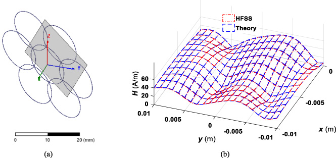
(a) Simulation setup in HFSS for verifying the H-field calculation, (b) comparison between simulated and calculated H-field.

In order to verify the calculation, a three-phase one-layer Tx coil array, including 7 circular coils with 7-mm radius, is simulated by the popular full-wave electromagnetic solver tool, HFSS (Ansoft, Pittsburgh, PA). The H-field at 4-mm target height (i.e. z = 4 mm) along the direction of 𝛽_Z = 45° and 𝛾 = 0° is inspected. The Tx coil array is assumed to have a 45° angle with respect to the x-axis in HFSS as shown in Fig. 6a. The H-field is recorded along the z-axis. The theoretical and simulated H-fields agree well within the range of −10 mm ≤ x ≤ 0 mm and −10 mm ≤ y ≤ 10 mm, as shown in Fig. 6b.

4. Optimizing Tx array coil dimensions

For the potential application of powering the arbitrarily distributed implants, shown in Fig. 2, the main goal of the Tx optimization is to create a strong homogeneous H-field. In reality, the positions where exists the minimum H-field easily result in the dead spots, being the bottlenecks of the system. Hence, improving the minimum H-field becomes the first priority in optimizing the Tx coil array. Equating the average or variance of all the H-field values, which is an indicator of the EM-field homogeneity, has the second priority. This optimization goal is very different from the traditional coil optimization that usually maximizes the PTE in the best case scenario [20], i.e. when the Rx and Tx coils are perfectly aligned. Here, elevating the worst-case PTE is the main purpose of the optimization.

The distance between the Tx coil array and the distributed implants is assumed to be about 20 mm [7], which includes a typical 1-mm of skin, 2-mm of fat, 7-mm of bone, 1-mm of dura matter, and 2-mm of the cerebrospinal fluid (CSF). Within this power transfer distance, the H-fields under various 𝛽_Z and 𝛾 values are computed using the equations presented in Section 3, while sweeping the radius of the circular coil. The H-field value at certain a location takes on the mean of the H-fields from all three layers. 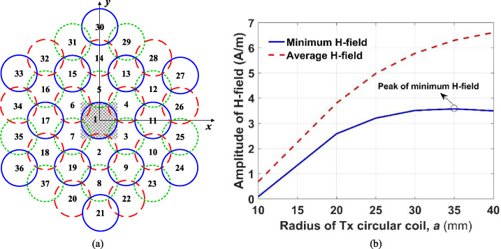The average of the H-field in the region of interest is H _{n_avg}, $\begin{eqnarray}\displaystyle H_{n\_\text{avg}}={\displaystyle \frac{\displaystyle \sum |A_{n\_1\_k}|+\displaystyle \sum |A_{n\_2\_k}|+\displaystyle \sum |A_{n\_3\_k}|}{3N_{\text{coil}}}}, & & \displaystyle\end{eqnarray}$ (6) where A _{n _ j _k} is the amplitude of effective H-field in (5) generated by the kth circular coil at the jth layer, and N _coil is the total number of the coils in one layer.

Fig. 7.

(a) Arrangement of 37 coils on one layer of the Tx coil array, and (b) calculated minimum and average H-fields versus the coil radius.

The coil arrangement in one layer is shown in Fig. 7a, where the solid blue line represents the 0° initial phase, the dashed red line represents the 120° initial phase, the dotted green line represents the 240° initial phase. The other layers are copied and moved from this layer with the relationships C _x2 = C _x1 − a∕2, C _y2 = C _y1 +3^0.5 a∕2, C _x3 = C _x1 + a∕2, and C _y3 = C _y1 − 3^0.5 a∕2, where C _xj and C _yj are the x- and y-coordinates of the coils at the jth layer, and all the coils have the same radius a. The hashed 2a × 2a square in the center of Fig. 7a is the inspected region. The number of coils on each layer is N _coil = 37 in this example.

The calculated results are shown in Fig. 7b where 0.5° angle-step is used for sweeping angles 𝛽_Z and 𝛾, and 1-mm position-step is used for sweeping the Rx coil positions. From Fig. 7b, one can observe that 35-mm is the optimal coil radius because the minimum value of the H-field reaches its maximum, although the average of the H-field is still increasing with the coil radius.

5. Experimental verification

Figure 8 shows the measurement setup that is constructed to verify the Tx coil array. The three-phase three-layer signal is generated by a FPGA board and transferred to a driver board to improve their driving ability before they are applied to the coil array. The Tx coil array and the Rx coil are held 2 cm apart with nonconducting materials.

Fig. 8.

Measurement setup for the Tx array.

5.1. Three-phase three-layer signal generator

The operating frequency is important for obtaining high quality factor [34]. In this paper, we focus on the distribution of the magnetic field, produced by the Tx coil array, which is not a function of frequency. For the millimeter-sized coils, the optimal operating frequency is on the order of 100 s of MHz [34]. On the Tx side, however, the coil size is in the centimeter scale, resulting in optimal frequency being around 10 s MHz [20]. In this prototype, 12.5 MHz was selected as the operating frequency because the optimization is being performed on the Tx coils.

The 50 MHz FPGA (EP4CE6F17C8, Altera) clock is multiplied by 3 using a built-in PLL to generate 150 MHz. The 150 MHz clock is then divided by 12 to obtain the 12.5 MHz operating frequency. The three different initial phases (0°, 120°, 240°) are realized by setting 26.67 ns (1/3rd of the period) delay between adjacent signals. The three coil layers are time division multiplexed by layer selection signal, each with 300-μs period and 1/3rd duty cycle, i.e. being high for 100 μs and low for 200 μs. The simulated three-phase and three-layer signals are shown in Figs 9a and b, respectively.

Fig. 9.

(a) Simulated three-phases signals, and (b) three-layer signals.

5.2. Driver and coil boards

Fig. 10.

(a) Hardware of the driver board, and (b) schematic of the driver board.

The hardware and the schematic of the driver board are shown in Fig. 10a and b, respectively, where the three-phase signals are input to three boards. The three-phase signals and three-layer signals are firstly synchronized by D-flip-flops. Two non-overlapping signals are further generated and applied to the current-mode class-D power amplifiers (PA).

The Tx coil array has been implemented on a PCB made of FR4, which is a woven fiberglass impregnated with an epoxy resin with permittivity of 4.4. The conductor material was copper with 35 μm thickness, commonly known as 1oz copper. Nineteen hexagonal coils with 35-mm side-length were included in each layer, as shown in Fig. 11. In measurements, each layer can be characterized independent of the others as long as the coils on the other layers are open-circuit.

Although 12.5 MHz has a 24 m wavelength, using long signal transmission interconnects introduce considerable phase shift that would degrade the PTE performance measurement results. This phase-shift generally impacts the Tx array in two ways that need to be considered. On the one hand, the phase-shift for the coils with the same initial phase (e.g. 120°) on one corner of the PCB array to the other corners should be minimized. In order to reduce this phase-shift, the coils with the same initial phase are divided into three groups and connected in parallel. On the other hand, the phase-shift difference between three signal paths with different initial phase (i.e., 0°, 120°, and 240°) should be minimized. This is ensured by designing the setup such that the transmission length would be almost the same for each signal path. The total transmission length can be fine-tuned by adjusting the length of the coaxial cables that are used to connect the driver boards to the Tx coil array. The total transmission length, including the coaxial cable length and the coil length, for each of the three signal paths in this setup was about 97 cm, as shown in Table 1.

Table 1

The total length of the transmission length for each part

Initial-phase	Path 1	Path 2	Path 3
0°	104 cm	97 cm	97 cm
120°	97 cm	97 cm	97 cm
240°	97 cm	97 cm	97 cm

Fig. 11.

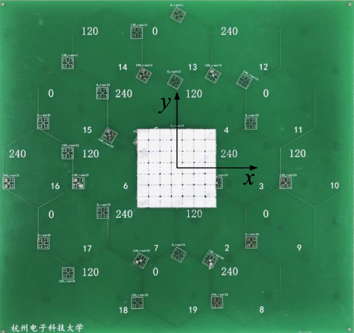
Photograph of the coil board.

5.3. Rx coil

The size of the Rx coil is desired to be as small as possible to minimize tissue damage particularly in the delicate area around the brain. On the other hand, according to Faraday’s law of induction, the induced voltage across the Rx coil is proportional to its size when the magnetic field produced by the Tx coil is constant, $\begin{eqnarray}\displaystyle {\varepsilon}=-N{\displaystyle \frac{d{\Phi}}{dt}}=-NS{\displaystyle \frac{dB}{dt}}=-NS{\mu}_{r}{\displaystyle \frac{dH}{dt}}, & & \displaystyle\end{eqnarray}$ (7) where ϵ is the induced voltage, N is the Rx coil number of turns, Φ is the magnetic flux that passes through the Rx coil. The magnetic flux is the product of the cross-section area of the Rx coil (S) and the magnetic field density norm to the cross-section (B), which is in turn proportional to the relative permeability of the environment that the Rx coil located in and the magnetic field strength (H). Therefore, the induced voltage (ϵ) is small because of the small size of the Rx coil. In our measurement setup, shown in Fig. 8, an oscilloscope is used to measure the induced voltage. Larger amplitude of the induced voltage is helpful in measuring the homogeneity of the distribution of magnetic field and reducing the measurement error above the noise floor. Because the focus of this work is on design of the Tx coil array, the Rx coil size is not necessarily optimized. However, as presented in [35,36], we expect to achieve even better PTE when Tx and Rx coils are optimized together. To facilitate handling, an Rx coil with 4 mm in diameter was chosen with 20 turns of insulated AWG 36 copper wire from TEMCo (Fremont, CA) with 0.15 mm in diameter, wound around a ferrite rod to further improve the induced voltage. The ferrite core, which is made of Material #61 from Fair-Rite Corp. (Wallkill, NY), has a relative permeability of ∼100. The effective relative permeability of a ferrite core (μ_{eff_r}) has been analyzed in [37 ], and can be expressed as ((8)) if the length (l _f) to diameter (2r _f) ratio, i.e. 𝜆 = l _f∕(2r _f) ≥1, $\begin{eqnarray}\displaystyle \begin{array}{@{}l@{}}\displaystyle {\mu}_{\text{eff}\_r}={\displaystyle \frac{{\mu}_{r}}{1+0.755D_{\text{fe}}{\lambda}^{0.13}({\mu}_{r}-1)}}\\[10.0pt] \displaystyle D_{\text{fe}}=(2r_{f}^{2}/l_{f}^{2}e^{3})\cdot [\ln (1+e/1-e)-2e]\\[5.0pt] \displaystyle e=\sqrt{1-1/{\lambda}^{2}},\end{array} & & \displaystyle\end{eqnarray}$ (8) where D _fe is the demagnetizing factor of an ellipsoidal ferrite [37]. Figure 12 shows the Rx coil of which connecting wires are twisted to minimize the induced voltage onto the loop of wire that forms between the Rx coil and its terminals and results in fluctuations in the induced voltage when the coil is moved.

Fig. 12.

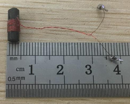
Photograph of the Rx coil.

Table 2

Three different measured cases

	Distance	𝛾	𝛽_Z
Case 1	2 cm	270°	0°
Case 2	2 cm	270°	45°
Case 3	2 cm	270°	90°

5.4. Experimental results

For simplicity but without loss of generality, a 7 × 7cm² area in the center of the coil array was selected to measure the magnetic field from 64 points at the height of 2 cm above the surface, as shown in Fig. 11. At each point, three typical cases with different orientation are measured, as shown in Table 2, where 𝛾 and 𝛽_Z are the angles shown in Fig. 5(b). Figure 13 shows an example of the measurement when 𝛽_Z =45°, 𝛾 =270°, and the distance is 2 cm. For each case and at each point, we measured the induced voltage 5 times and averaged them to reduce the error that is induced by manual positioning.

Fig. 13.

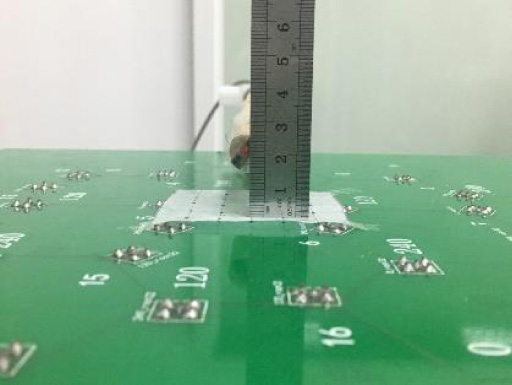
Measurement setup at different orientation of Rx coil.

The measured results for one-layer three-phase Tx array with different 𝛽_Z angles (𝛽_Z = 0°, 𝛽_Z = 45°, and 𝛽_Z = 90°) are shown in Fig. 14a. When 𝛽_Z = 0°, it is a convex shape. When 𝛽_Z = 90°, if the Rx coil is above x-axis, i.e. y = 0, the received voltage is minimum. For these two cases, the shapes are roughly symmetrical about x-axis or y-axis. When 𝛽_Z = 45°, the received voltages for the region of y <0 are larger than those for the region of y > 0. The shape is not symmetrical about y-axis anymore.

As a comparison, the measured results for one-layer in-phase Tx array are also given (Fig. 14b). Both Tx arrays in Figs 14a and 14b are comprised of 35 mm side-length hexagonal coils but with different excitation currents. From Fig. 14, it can be seen that received voltages from the in-phase Tx array is much smaller than those from the three-phase Tx array. That is due to the current cancellation effect in the in-phase Tx array, as explained in Section 2. In each subfigure of Fig. 14, the standard deviation and the average voltage value calculated from the data plotted in each subfigure are marked. Although the standard deviations in Fig. 14a are much larger than those in Fig. 14b, the average values for one-layer three-phase Tx array are improved by ∼70% compared to that of in-phase Tx array (see Table 3). The fluctuation in the received voltage in Fig. 14a (i.e., the high standard deviation) are expected to become more smooth when the three layers are activated (See Fig. 15).

Fig. 14.

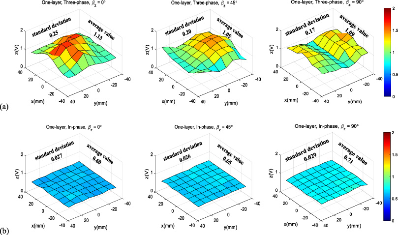
Measured induced voltage of the Rx coil at different orientation and location for one-layer Tx array: (a) three-phase, (b) in-phase.

Table 3

Measured average voltages

Side-length of hexagonal coils	𝛽_Z	In-phase one-layer	In-phase three-layer	Three-phase one-layer	Three-phase three-layer	% increasement of three-phase three-layer compared to in-phase three-layer
10 mm	0°	0.59 V	0.62 V	1.03 V	1.09 V	84.7%
	45°	0.48 V	0.52 V	0.86 V	0.91 V	89.6%
	90°	0.38 V	0.39 V	0.43 V	0.45 V	18.4%
20 mm	0°	0.65 V	0.65 V	1.10 V	1.14 V	75.4%
	45°	0.57 V	0.59 V	0.98 V	1.05 V	84.2%
	90°	0.57 V	0.55 V	0.73 V	0.75 V	31.6%
35 mm	0°	0.60 V	0.63 V	1.13 V	1.19 V	98.3%
	45°	0.65 V	0.63 V	1.05 V	1.09 V	67.7%
	90°	0.71 V	0.72 V	1.09 V	1.17 V	64.8%

The measured results for three-layer three-phase Tx array with 10 mm, 20 mm, and 35 mm hexagonal coils side-length are compared in Figs 15a–c, respectively. By comparing Fig. 15c with Fig. 14a, we can observe that the measured voltages for three-layer Tx array are smoother than those for one-layer Tx array, although the maximum voltages for three-layer Tx array are decreased slightly because they are the average values from three time-multiplexed Tx layers. The standard deviation values are decreased from 0.17–0.25 in Fig. 14a to 0.06–0.08 in Fig. 15c. At the same time, the average values are slightly improved from 1.05–1.13 V in Fig. 15a to 1.09–1.19 V in Fig. 15c. From Fig. 15, we can also find that the Rx coils received voltages are increased with the side-length of the hexagonal coils especially when 𝛽_Z =0°. The average measured voltages for one- or three-layer, in- or three-phase Tx array with different side-length hexagonal coils are summarized in Table 3. Considering the total area of the Tx coil in applications, such as wirelessly energizing the implanted neural recording devices, larger side-length are not practical. From Table 3, we can find that the average voltages are improved for three-phase Tx array compared to the in-phase Tx array. The final column in Table 3 shows the increasement of the values of the three-phase three-layer case compared to the in-phase three-layer case. The conclusion about the average voltage from Fig. 15 and Table 3 is consistent with the analysis shown in Fig. 7(b).

Fig. 15.

Measured induced voltages of the Rx coil at different orientations and locations for three-layer Tx array with (a) 10 mm, (b) 20 mm, and (c) 35 mm side-length of hexagonal coils.

Besides the average voltage, the minimum voltages for these cases are also extracted from the measured data and summarized in Table 4. As expected, the minimum voltages are improved for three-phase three-layer Tx array compared to the in-phase Tx array or three-phase one-layer Tx array.

Table 4

Measured minimum voltages

Side-length of hexagonal coils	In-phase one-layer	In-phase three-layer	Three-phase one-layer	Three-phase three-layer	% increasement of three-phase three-layer compared to in-phase three-layer
10 mm	0.26 V	0.26 V	0.29 V	0.34 V	30.8%
20 mm	0.46 V	0.46 V	0.51 V	0.63 V	37.0%
35 mm	0.54 V	0.59 V	0.70 V	0.83 V	53.7%

6. Discussion

The method of optimizing the side-length of hexagonal coils in this paper is based on 20-mm distance between the Tx array and the Rx coil. In a specific application, the optimization results can be updated by using the method proposed in this paper. Some limitations in our design still exist.

Firstly, the structure of the Tx coil array should be studied furthermore. Although the Tx coil array is extendible and the coverage area is not limited, the solid PCB coil array has different transmission distances to the Rx coils because of the uneven brain shape. In future work, the property for different transmission distance will be further studied. The Tx array printed on flexible substrates will be studied, optimized, and fabricated to match the shape of the brain. The flexible Tx array that can conform to the human head like a hat and will reduce the transmission distance which generally improves the power transfer efficiency especially for the Rx coils at the brain region where it is not the central.

Secondly, from the perspective of the optimization for the system, the parameters PTE, PDL, and SAR, the Rx coils, and the operating frequency should be considered together. Because of the weak coupling between the Tx coils and the Rx coils, the Tx and Rx coils can be designed separately [36]. The main objective in Tx coil design is creating the homogeneous H-field around the Rx coil, which is the study in this work. The main objective in the Rx coil optimization, however, is capturing maximum induced power at resonance and delivering it to the load, which is the study in [36]. The PTE of the system from DC power to the load needs to be considered in future. The PTE of the system is different from the traditional PTE of coupling link i.e., PTE from single Tx coil to single Rx coil. In general, the PTE of this design will be much lower than the PTE from single Tx coil to single Rx coil at the best case scenario with Tx and Rx coils coaxially oriented. However, the PTE of this design is comparable even better than the PTE from single Tx coil to single Rx coil at the worst case scenario with Tx and Rx coils coaxially and perpendicularly oriented.

For the SAR parameter, SAR = σ|E|²∕𝜌, where σ and 𝜌 are the tissue conductivity and density, respectively, E is the electrical field strength, is limited under 1.6 W/kg [15]. According to the analysis in [20] and [36], the SAR limitation is “mainly determined by the Tx coil design” [36]. That is because the E-filed around the Rx coil inside the tissue is low enough compared to the E-filed around the Tx coil. This safety limit can be satisfied by adopting method like segmentation of the Tx coil [20,38]. In addition, the method to produce homogeneous H-filed for the Rx coils improves the uniformity in the E-field of Rx coils and reduce the risk of exceeding SAR limit. In traditional WPT system design, the system is usually optimized for the best case scenario as mentioned previously. That is to say, if the Rx coils in the worst case should be ensured to receive enough power, the Rx coils in the best case will receive much more power than the required power, which easily results in exceeding SAR limit.

The PDL depends on the specific load resistance, PTE, Tx power, and SAR limitation. If the specific load is given (e.g., 1 k𝛺) in specific application, the PDL can be calculated according to the induced voltage. The PDL is mainly related to the design of Rx coils if the homogeneous H-filed around the Rx coils has been designed.

The distribution of H-field from the Tx coils is related to the operating frequency as long as the operating frequency is not too high. However, the phase-shift of the excitation current going through the coil will increase with the frequency, which has been considered in the manuscript. For the Rx coil, the quality factor and the permittivity of the coating material and the tissue are strongly related to the operating frequency [36]. So, the operating frequency should be selected from based on the optimization of Rx end. At the same time, the phase-shift of the excitation current should be considered when the selected frequency is high enough.

7. Conclusions

In this paper, to address the problem of powering distributed fully-implanted neural recording devices, a three-phase three-layer TX coil array is designed. The coil size is optimized by calculating the magnetic field produced by the Tx coil array. A prototype is constructed to verify the design. According to the measurement results, the new Tx coil array design can generate more homogeneous and larger magnetic field distribution, compared to the traditional approach.

Footnotes

Acknowledgements

The authors gratefully acknowledge the support of the Zhejiang Provincial National Natural Science Foundation of China under Grant No. Z20F010015, and the National Natural Science Foundation of China under Grant No. 61771175. The authors gratefully acknowledge the discussion with Byunghun Lee at Incheon National University.

References

Nicolelis

, Actions from thoughts, Nature 409(6818) (2001), 403–407.

Hochberg

Bacher

Jarosiewicz

, Reach and grasp by people with tetraplegia using a neurally controlled robotic arm, Nature 485(7398) (2012), 372–375.

McConnell

G.C.

Rees

H.D.

Levey

A.I.

Gutekunst

C.-A.

Gross

R.E.

and Bellamkonda

R.V.

, Implanted neural electrodes cause chronic, local inflammation that is correlated with local neurodegeneration, J. Neural Eng. 6 (2009), 056003.

BRAIN initiative, Available online: http://www.whitehouse.gov/share/brain-initiative.

Biederman

Yeager

Narevsky

Koralek

Carmena

Alon

, A fully-integrated, miniaturized (0.125 mm²) 10. 5 μW wireless neural sensor, IEEE J. Solid State Circuits 48 (2013), 960–970.

Lee

Mok

Huang

An implantable wireless network of distributed microscale sensors for neural applications, in: 9th Intern. IEEE/EMBS Confer. Neur. Engin. (NER), San Francisco, USA, 2019, pp. 871–874.

Cheng

Wang

and Ghovanloo.

, Analytical modeling and optimization of small solenoid coils for mm-sized biomedical implants, IEEE Trans. Microw. Theor. Tech. 65 (2017), 1024–1035.

Cheng

Qian

Chen

Sun

and Wang

, Sensitivity analysis of L-type impedance matching circuits for inductively coupled wireless power transfer, Intern. J. Appl. Electro. Mechan. 61(1) (2019), 1–11.

Philip

Santis

V.D.

and Li.

, Driving range of electric vehicles charged by wireless power transfer, IEEE Trans. Vehic. Techn. 69 (2020), 5968–5982.

10.

Brizi

Stang

J.P.

Monorchio

and Lazzi

, A compact magnetically dispersive surface for low-frequency wireless power transfer applications, IEEE Trans. Antenn. Propag. 68 (2020), 1887–1895.

11.

Song

S.H.

Kim

and Ziaie

, Omnidirectional ultrasonic powering for millimeter-scale implantable devices, IEEE Trans. Biomed. Eng. 62 (2015), 2717–2723.

12.

Kim

and Park.

, Optimization of optical wireless power transfer using near-infrared laser diodes, Chin. Opt. Lett. 18 (2020), 042603.

13.

Montgomery

K.L.

, Wirelessly powered, fully internal optogenetics for brain, spinal and peripheral circuits in mice, Nature Methods (2015), 969–974.

14.

Murphy

M.D.

Guggenmos

D.J.

Bundy

D.T.

and Nudo

R.J.

, Current challenges facing the translation of brain computer interfaces from preclinical trials to use in human patients, Frontiers in Cellular Neuroscience 9 (2016), 497.

15.

IEEE Recommended Practice for Measurements and Computations of Radio Frequency Electromagnetic Fields With Respect to Human Exposure to Such Fields, 100 kHz–300 GHz, IEEE Standard C95.3-2002 (R2008), 2002.

16.

Zhang

Liu

Jiang

, Near-field wireless power transfer to deep-tissue implants for biomedical applications, IEEE Trans. Antenn. Propag. 68 (2019), 1098–1106.

17.

Kurs

Karalis

Moffatt

, Wireless power transfer via strongly coupled magnetic resonances, Science 317(5834) (2007), 83–86.

18.

Zargham

and Gulak

, Maximum achievable efficiency in nearfield coupled power-transfer systems, IEEE Trans. Biomed. Cir. Syst. 6 (2012), 228–245.

19.

Dai

, Maximum efficiency tracking for wireless power transfer systems with dynamic coupling coefficient estimation, IEEE Trans. Pow. Electron. 33 (2017), 5005–5015.

20.

Mirbozorgi

S.A.

Yeon

and Ghovanloo

, Robust wireless power transmission to mm-sized free-floating distributed implants, IEEE Trans. Biomed. Circ. Syst. 11 (2017), 692–702.

21.

Shi

and Smith

J. R.

, Large area wireless power via a planar array of coupled resonators, in: IEEE International Workshop on Antenna Technology (iWAT), Cocoa Beach, FL, USA, 2016, pp. 200–203.

22.

Liu

Chen

Guo

A novel multi-coil magnetically-coupled resonance array for wireless power transfer system, in: IEEE Wireless Power Transfer Conference (WPTC), Taibei, Taiwang, 2017, pp. 1–3.

23.

Wang

Q.H.

Gao

Mao

and Sun

, A novel mat-based system for position-varying wireless power transfer to biomedical implants, IEEE Trans. Magn. 49 (2013), 4774–4779.

24.

Liu

Guo

Jolani

Planar magnetically-coupled resonance wireless power transfer systems using array of coil resonators, in: IEEE MTT-S International Wireless Symposium (IWS), Shanghai, China, 2016, pp. 1–3.

25.

Park

Lee

Cho

G. H.

, Two-dimensional inductive power transfer system for mobile robots using evenly displaced multiple pickups, IEEE Trans. Indust. Appl. 50 (2014), 558–565.

26.

Ahn

Park

H.H.

Choi

C.S.

Reduction of electromagnetic field (EMF) of wireless power transfer system using quadruple coil for laptop applications, in: IEEE MTT-S International Microwave Workshop Series on Innovative Wireless Power Transmission: Technologies, Systems, and Applications (IMWS), Kyoto, Japan, 2012, pp. 65–68.

27.

Sonntag

C.L.W.

Lomonova

E.A.

and Duarte

J.L.

, Power transfer stabilization of the three-phase contactless energy transfer desktop by means of coil commutation, in: IEEE Young Researchers Symposium in Electrical Engineering, Eindhoven, The Netherlands, 2008, pp. 1–6.

28.

Lee

Ahn

and Ghovanloo

, Three-phase time-multiplexed planar power transmission to distributed implants, IEEE J. Emerg. Select. Top. Power Electron. 4 (2016), 263–272.

29.

Russell

McCormick

Taberner

Wireless power delivery system for mouse telemeter, in: IEEE Biomed. Circ. Syst. Conf., Beijing, China, 2009, pp. 273–276.

30.

Cheng

Chen

Qian

Optimizing three-phase three-layer coil array for omnidirectional wireless power transfer, in: IEEE Wireless Power Transfer Conference (WPTC), Taibei, Taiwang, 2017, pp. 1–3.

31.

Cheng

and Shu.

, A new analytical calculation of the mutual inductance of the coaxial spiral rectangular coil, IEEE Trans. Magn. 50 (2014), 7026806.

32.

Good

R.H.

, Elliptic integrals, the forgotten functions, Eur. J. Phys. 22 (2001), 119–126.

33.

Abramowitz

and Stegun

I.A.

, Handbook of Mathematical Functions with Formulas, Graphs, and Mathematical Tables, 9th edn, Dover, New York, 1972.

34.

Moradi

Amendola

Björninen

Sydänheimo

Carmena

J.M.

Rabaey

J.M.

, Backscattering neural tags for wireless brain-machine interface systems, IEEE Trans. Antenn. Propag. 63 (2015), 719–726.

35.

Ahn

and Ghovanloo

, Optimal design of wireless power transmission links for millimeter-sized biomedical implants, IEEE Trans. Biomed. Cir. Syst. 10 (2016), 125–137.

36.

Cheng

Wang

and Ghovanloo.

, Analytical modeling and optimization of small solenoid coils for mm-sized biomedical implants, IEEE Trans. Microw. Theory Techn. 65 (2017), 1024–1035.

37.

Theilmann

P.T.

and Asbeck

P.M.

, An analytical model for inductively coupled implantable biomedical devices with ferrite rods, IEEE Trans. Biomed. Cir. Syst. 3 (2009), 43–52.

38.

Stoecklin

Yousaf

Gidion

, Efficient wireless power transfer with capacitively segmented RF coils, IEEE Access 8 (2020), 24397–24415.