
Abstract
Eddy current testing is widely used for the automatic detection of defects in conductive materials. However, this method is strongly affected by probe scanning conditions and requires signal analysis to be carried out by experienced inspectors. In this study, back-propagation neural networks were used to predict the depth and length of unknown slits by analyzing eddy current signals in the presence of noise caused by probe lift-off and tilting. The constructed neural networks were shown to predict the depth and length of defects with relative errors of 4.6% and 6.2%, respectively.
Introduction
Non-destructive testing (NDT) methods play a critical role when inspecting for defects in various industrial components. NDT comprises a group of techniques used to evaluate and characterize materials without changing their original properties [1]. Of these techniques, eddy current testing (ECT) is widely used for testing the structural health of conductive materials used in the power industry, machinery, and aircraft. Based on the principle of electromagnetic induction, ECT has experienced several decades of development and is frequently used for the detection and sizing of defects on or near the surface of conductive materials. It has many advantages, including economical and simple operation, and can be used to construct an automated scanning system for rapid detection. However, ECT is very sensitive to perturbations in scanning conditions mainly caused by probe lift-off and tilting, which can significantly increase the noise in the detected signal [2]. Therefore, ECT must be performed by experienced inspectors to ensure its speed and accuracy, which would substantially limit the efficiency of the fast ECT detection system and the accuracy of dimension analysis. For this reason, an automatic dimensional analysis model is highly desirable to guarantee accurate analyses even in the presence of significant noise.
Artificial intelligence and big data analysis have led to new developments in ECT methodology. Several groups have proposed methods to automatically analyze ECT signals using machine learning theory, such as decision trees, support vector machines, and neural networks. Neural networks have received particular attention because of their superior performance [3]. A neural network was used to evaluate eddy current signals and found to be reliable at simultaneously predicting the depths and angles of cracks according to the extracted features [4]. Another study showed that a new extreme-learning machine model using the kernel-based principal component analysis algorithm could extract the features of ECT signals and neural networks were used to realize defects classification and quantitative analysis [5]. However, these studies did not consider the noise effect, which is a critical factor affecting ECT, and the feature extraction process is too complicated to improve the signal analysis efficiency. In the actual detection process, noise such as that caused by lift-off of the probe has a non-negligible influence on the characteristics of signal features. This noise makes the extraction of those features more difficult, leading to erroneous conclusions. Simultaneously, simple data analysis and feature extraction remain desirable.
Different scanning conditions can produce signals containing different information. Therefore, in the present study, two scanning paths are used to collect depth and length signals and provide more accurate results. Based on the raw ECT signals affected by probe lift-off and tilting, two back-propagation neural networks (BPNNs) are introduced to quantitatively predict the depth and length of slits. The ECT signals are collected by experiment and simulation. The constructed BPNNs are then trained using collected training data, and the performance of the trained neural networks are evaluated against a panel of test samples.
Data acquisition
To obtain and reliably evaluate comprehensive data, the eddy current signals were produced experimentally and also simulated.
Experiment
The ECT signals were acquired using the system shown in Fig. 1. The ECT probe was a self-induced differential probe with two air-core coils. The detection coil and the reference coil were wound in a cylindrical shape with 750 turns. The specimen, whose electrical conductivity was 1.33 × 10⁶ S/m6, was manufactured with AISI 316 stainless steel. Three 15 mm × 0.3 mm rectangular slits with different depths (0.5, 1, and 2 mm) were fabricated on the specimen using electrical discharge machining (Fig. 2). The excitation signal was generated using an ASWAN-ASSORT PC, which can simultaneously generate three different signal frequencies between 1 kHz and 1.8 MHz. The measurement software, based on the LabVIEW environment, allowed automatic detection by controlling a two-dimensional scanning mechanism. The software stored the signals collected using a data acquisition instrument.
In this study, the probe was placed on the specimen and scanned along two paths (to collect depth and length signals) (Fig. 3). Using a constant scan pitch of 0.2 mm per step, the probe was scanned perpendicular to the slit length, passing through the slit center (Fig. 3a), and scanned along with the slit length (Fig. 3b). During the scanning process, the excitation frequencies were varied from 50 kHz to 100 kHz. A fixed scan distance of 40 mm was used, with the slits being placed in the middle of the scanning path. In addition, the noise caused by probe lift-off and probe tilting was artificially introduced (Fig. 4). Two different 40 mm scan paths were used to collect depth and length signals. For the scan paths shown in Fig. 3a and 3b, the noise was introduced at a distance of 10 mm and 15 mm, respectively, from the midpoint of the scan. Probe lift-off was introduced by raising the probe during the scanning process, the lift-off distance being defined by the distance between the probe tip and the surface of the specimen. Probe tilting was introduced by rotating the arm of the scanning mechanism to create an angle between the probe tip and the surface of the specimen. The lift-off distance and the tilting angle were set to ca. 2 mm and 3 degrees, respectively. As a control, the same measurements were also performed using a specimen of AISI 316 stainless steel free from defects.
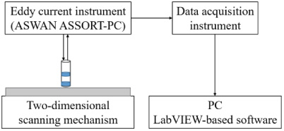
Block diagram of ECT system.
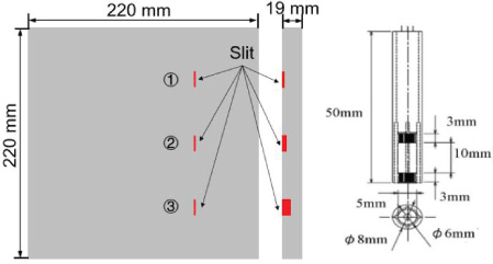
Structure diagram of specimen (left) and probe (right).
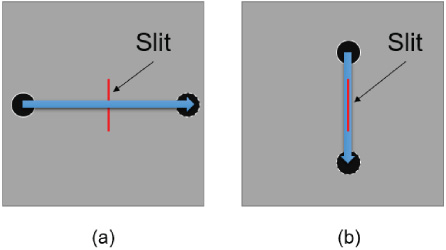
Diagram of two scan paths.
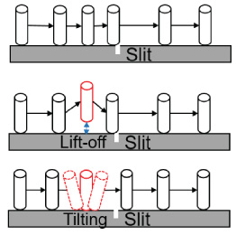
Scan conditions with and without noise.
Sizes of slits in experiment and simulation
ECT signals were emulated using the CIVA software, a dedicated simulation platform for non-destructive testing techniques [7]. Models of the specimen and the probe used in the experiment were constructed. The probe model comprised two air-core coils having the same performance parameters as the experimental coils. The specimen model consisted of one rectangular slit, with the variable slit size and the physical properties (such as electrical conductivity and relative permeability) of the AISI 316 stainless steel being set in CIVA. The simulated scan distance and pitch were identical to the experimental parameters. A comparison of the experimentally-determined and simulated slit dimensions for the two scanning paths shown in Fig. 3 is given in Table 1. The simulated ECT signals cannot be affected by environmental factors, such as experiment temperature and vibration of the scanning mechanism, and are not affected by noise (lift-off and tilting) during the simulated scanning process. Because they used the same scan distance and scan pitch, the experimental and simulated ECT signals have the same number of data points. Therefore, the noise measured during the experimental scans of the defect-free specimen was added to the noise-free simulation signals.
Signal normalization
Collected data were processed in accordance with the JEAG 4217-2010 guideline for eddy current measurement using a surface coil [8]. Specifically, the maximum amplitude of the Lissajous waveform of a 1 mm slit was amplified to 1 V, and the phase of each frequency was rotated by 90° (Fig. 5a). Collected signals of the same frequency were processed using the same amplification and rotation coefficients.
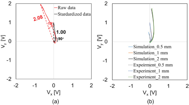
Diagram of (a) standardization process and (b) comparison results of simulation and experiment data.
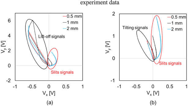
The Lissajous figures of slit signals with (a) lift-off and (b) tilting from experiment.
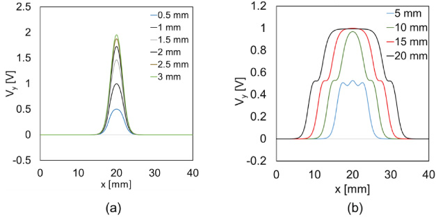
Diagram of (a) different depth slit signals and (b) different length slits signals from simulation.
The comparison of simulation data and experiment data is implemented by three different depth slits (0.5 mm, 1 mm and 2 mm), and the results are shown as Fig. 5 (b). For the 1 mm results, the simulation data and experiment data have the same amplitude due to the same normalization process. According to the Lissajous figures, it is evident that the simulation signals have the same characteristics as experiment data. From the 0.5 mm and 2 mm signals, the phases of experiment data and simulation data are nearly the same. However, the amplitudes are slightly different. The maximum amplitude values of the experimental 0.5 mm and 2 mm signals are 0.42 V and 1.76 V, respectively. And the maximum amplitude values of the simulated 0.5 mm and 2 mm values are 0.49 V and 1.75 V, respectively. In conclusion, the simulation data collected by CIVA is consistent with the experiment data.
As shown in Fig. 6, the signals corresponding to noise produced by lift-off and tilting have different phase characteristics from the signals associated with the slits. The curve features are also different, with the lift-off signals and tilting signals being closer to a straight line because the noise was caused by sudden changes. The signals produced in response to probe lift-off and tilting have similar phase characteristics, while the amplitude characteristics are different. The maximum signal amplitude caused by probe lift-off is much larger than the maximum amplitudes caused by probe tilting and slit traversal. And the maximum amplitude of tilting signals is nearly equal to the amplitude of 1 mm depth slit signals. The relationships between slits having different depth and length are shown Fig. 7, indicating that deeper slits are seen to have larger values of V y (Fig. 7a) and longer slits have a wider amplitude range (Fig. 7b). Therefore, it is desirable to establish the mentioned functional relationships using neural networks to automatically predict the depth and length.
The BPNN is a supervised method involving several separate layers, including an input layer, an output layer, and hidden layers. In each layer, there are a number of processing nodes that receive inputs from nodes in the lower layers, and the nodes apply the transfer functions to their inputs to produce a single output. Each interconnection between two processing elements has an associated weighting factor that can be appropriately adjusted using a back-propagation training algorithm. Back-propagation is the key feature of neural net training and involves fine-tuning the weights of a neural network based on the error rate obtained in the previous epoch. Proper tuning of the weights ensures lower error rates, making the model more reliable by increasing its generalization.
Depth validation results of samples
Depth validation results of samples
Length validation results of samples
As mentioned above, the purpose of the BPNN is to establish the functional relationship between the ECT signal amplitude and depth of the slit. To reduce the training time, signal amplitudes were expressed only in terms of the V y component. Based upon the scan pitch and scan distance used in this study, one ECT signal consisted of 201 data points and hence the number of nodes in the input layer was the same. Because the output layer had only one value (depth of slit), there was one node in the output layer. During the design of the BPNN, one seeks to determine the number of nodes in the hidden layer. If there are too few hidden nodes, the relationship will be underdetermined, while too many hidden nodes may lead to over-fitting the problem. The selection of the number of hidden layers currently lacks a theoretical basis and is empirically determined based on experience and usage [9]. In this study, the number of neurons in the hidden layer is set as 20, which shows the best performance in comparison of other numbers. The training data set consisted of experimental and simulated data totaling 144 groups. For the neural network, function selection is essential and opportune functions can produce more reliable results. Because raw signals were used as feature characteristics, the Bayesian algorithm was used as the training function, resulting in good generalization for noisy datasets. The mean square error was chosen as a cost function, making the training process more accurate. Both experimental and simulated data were used to train the BPNN.
After many training runs and repeated screening, a training network was selected as the optimal network model. This model was validated using experimental test samples (1–15) that were scanned under the same conditions but differed from the training data because of the different environmental factors. The simulated test samples consisted of signals from slits of the same depth under different conditions (16–21) and signals from slits of different depth under the same conditions (22–27).
As shown in Table 2, the average relative error across the entire data set was 6.2% and it is evident that the trained neural network can predict the depth of the unknown slit, even in the presence of noise. Among the experimental test samples, the most significant relative error was 22%, corresponding to an absolute error of 0.11 mm, which is acceptable. The average relative error of the network model was 3.9%. The largest error is likely to be caused by the change of environment during the experiment, although parameter optimization and function selection of the BPNN will also affect the prediction accuracy. In simulation testing samples (16–21), the errors were smaller than 11%. It is evident that the trained BPNN can correctly predict the depth of the defect without being affected by the scanning conditions. For simulation testing samples (22–27), the most significant error was 18%, which shows that the BPNN has good accuracy and generalization ability. However, the error of 3.3 mm depth slit signals is significant because the maximum depth is 3.0 mm in training data. It can be concluded that the BPNN has the generation ability to predict the data, which is out of the range of training data.
Length prediction neural network
Because of the different relationship between amplitude and length, a new BPNN is used to achieve the relationship mapping. The input data also use V y signals, and the input layer is 201 neurons because of the same scanning condition. The output layer is one neuron, which shows the length of the slit. The hidden layer contains 18 neurons according to the performance comparison. The training data consist of experiment data and simulation data. The total number of training data is 48 groups. The same functions are selected to construct the length prediction BPNN. Similarly, the verification experiment is implemented using both experimental data and simulation data, and the results are shown in Table 3.
The whole average relative error was 6.2%, and the results show that the trained BPNN can accurately predict the length of unknown slit even in the presence of noise. The average error of experimental test samples (1–6) was 3.0% and the average error of simulated samples (7–18) was 8.3%. These results suggest that the BPNN performs well when making simple predictions of slit sizes. However, insufficient leaning data resulted in lower accuracy in comparison depth predictions.
Conclusions
This study implemented a BPNN method for the sizing of defects. There is no accurate formula and mathematical model to describe the relationship between the defect size and the ECT signal because of the complicated scanning conditions. In this study, the BPNNs were trained using the sizes of slits and raw ECT signals to map the relationships. The trained BPNNs could predict the depth and length of unknown slits, even in the presence of noise. The average relative errors in depth and length prediction were 4.6% and 6.2%, respectively. Besides, BPNNs could analyze lots of signals simultaneously.
Compared with the traditional signal analysis model, this method is more portable and adjustable. However, the BPNNs have a one-to-one correspondence with the training set, meaning they can only quantitatively analyze slit-shaped defects. Different types of defects have different signal characteristics, and future work will expand the automatic analysis system of multiple defects using the neural networks.
Footnotes
Acknowledgements
This work was supported in part by the Collaborative Research Project of the Institute of Fluid Science, Tohoku University.