Fast reconstruction of the magnetization of a Halbach magnet in EMAT using experimental measurements

1. Introduction

In electromagnetic acoustic transducers (EMAT) periodic permanent magnets in combination with coils are used to generate ultrasonic waves [1]. EMAT performance can be enhanced when a Halbach magnet system is employed, due to increased magnetic field distribution focused in one direction, but the complexity of the EMAT signal is increasing and further design optimizations of the sensor requires a detailed knowledge of Halbach magnetic field distribution. In EMAT, the Halbach magnet is composed from a combination of parallelepiped unit blocks with magnetization aligned in vertical or horizontal direction (Fig. 1). Experimental measurements indicate that EMAT performance (signal/noise ratio) depends also on the uniformity of magnet field distribution. While in a simplified approach a constant magnetization model can be employed for each unit block, experimental measurements of Halbach array shows the non-uniformity of the magnetic field distribution. Therefore it is not possible to compute accurately Halbach magnetic field without knowing the model distribution of magnetization of each block unit. While only reconstruction of magnetization of block units, and not Halbach array, with very high accuracy (<1%) were previously reported, they are very complex and based on inverse problems analyses using combination of 3D FEM-BEM (finite-boundary element). To increase the accuracy of open-boundary in large scale problems simulations models are combined with regularization methods based on Tikhonov or L-curve techniques to reduce the illness of inverse problem in finding the magnetization model of magnet [2].

In the present paper is reported a fast reconstruction method of the magnetization model of Halbach array magnet using experimental measurements of the magnetic field distributions (only the main component) outside of an individual magnet unit in the Halbach array, through the use of an adaptive incremental variation of magnetization in magnet division cells based on theoretical 2D/3D formula validated through 2D/3D FEM simulations. Also, the paper shows the feasibility of the method to reconstruct the magnetization model of an Halbach array composed of several magnet units, when measurements are conducted for Halbach magnet configuration, and not only for the individual magnet blocks. However, in the present paper the magnetization model reconstruction inside block magnet or Halbach array is limited to only one component of magnetization (main component) that is perpendicular to the surface of unit block or Halbach array with strongest flux distribution.

OPEN IN VIEWER

Fig. 1.

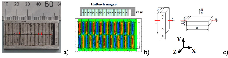
(a) View of the Halbach magnet composed through arrangement of H and V-block block magnets; (b) Distribution of H and V-blocks and magnetic flux density measurement above the Halbach magnet; (c) Geometry of H and V-blocks.

The accuracy of EMAT signal depends strongly on the performance of the magnet (magnetic field amplitude and uniformity) used to generate ultrasonic waves. Higher amplitudes of magnetic flux distributions are obtained using Halbach magnet arrays (Fig. 1). A periodic arrangements of horizontal (H) and vertical (V) block magnets, with magnetization oriented perpendicular to each other in each unit block, creates a higher magnetic field focused above surface of Halbach array than a standard periodic permanent magnetic array. The geometrical and magnetic parameters of H and V-blocks are described in Table 1. Experimental measurements were conducted to measure an individual unit magnet block (made of Sm-Co) or the full Halbach array using a Gauss-meter HGM-8300. The measurements of the magnetic flux distributions were recorded only for one component (perpendicular on the surface of magnet unit or Halbach array in Y-direction, with the strongest magnetic perpendicular flux density) at a 0.45 mm lift-off above magnet surface, with high accuracy. The thickness (0.35 mm) of magnetic probe was taken into account to estimate the magnetic probe lift-off, integrating the magnetic flux density in the sensor region of size of 0.07 × 0.07 mm². The unevenness of the magnet surface of magnetic blocks is small and was not considered in the present paper. As is shown in Fig. 1, the measurement of magnetic flux distribution of the Halbach magnet reveals a non-uniform pattern of magnetization due to the non-uniformity of the individual magnetization in block-magnets in the array. While the manufacturer data provides only a reference medium value of the main magnetization and not individually for each unit block, it was found through detailed measurements that their maximum amplitude values can differs up to 20% or even 30% and larger for limited samples. While it can be assumed that each magnetic block has a constant main magnetization component, experimental measurements of the magnetic flux distribution shows a different reality for H-blocks magnet. The disagreement with experimental measurements is stronger (for H-blocks) when a constant magnetization model (or unit relative magnetic permeability) is employed, as shown in Fig. 2.

The 2D model, both simulated by FEM or theoretical formula [3,4], was found to not be in good agreement with measurements. Only the simulations based on a 3D FEM or 3D theoretical formula (validated also for μ _r > 1), based on relative magnetic permeability slightly higher than air (∼1.05 as indicated in literature for magnets) agrees relatively well with measurements. However, both 2D/3D FEM showed (Fig. 2b) that only a non-uniform magnetization inside of magnet block is equivalent with a value of relative magnetic permeability slightly larger than one. While the 3D simulation/formula results in Fig. 2a agrees well with measurements on the median line above the magnet, it starts to disagree gradually stronger as the measurement line move toward the edge of the magnet, indicating that magnetization model is not constant across magnet surface for magnet block.

OPEN IN VIEWER

Fig. 2.

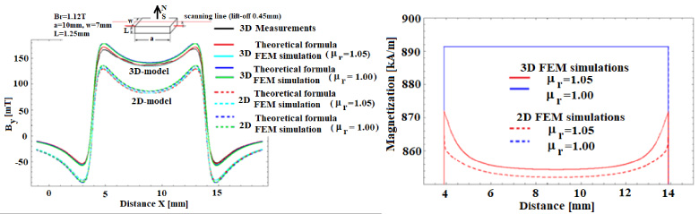
Comparison between measurements of B _y , 2D/3D FEM simulation and theoretical formula for H-block (left figure); H-block magnetization simulation by 2D/3D FEM with μ _r = 1, 1.05 (right figure)

The paper considered only the reconstruction of one main component of the magnetization of the magnet (in Y-direction as shown in Fig. 1a) across magnet surface X-Z. Figure 3 shows the experimental measurements (magnetic flux distribution in 3933 = 69 × 57 measurements points distributed 0.25 mm apart from each other over magnet surface) conducted above the H-block unit with a 0.45 mm lift-off. Small features of the flux distribution above the surface of magnet and near magnet edge, demonstrates the non-uniformity of magnetization model of the parallelepiped magnet.

OPEN IN VIEWER

Fig. 3.

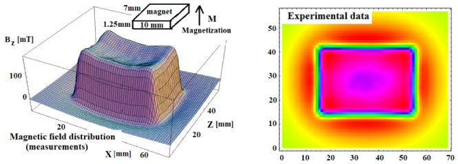
3D plot and contour lines of measurement of magnetic flux distribution above H-block magnet.

In order to reconstruct the magnetization model of the parallelepiped magnet a simple iterative algorithm was adopted to increase incrementally the magnetization of each magnet cell that results from division of magnet block in smaller equal parts defined by magnet mesh division (n _x − n _y − n _z ), as shown in detailed in Fig. 4. The magnetization of each cell is increased or decreased by a small value ΔM in order to assure the convergence of the iterative algorithm, but large enough to assure fast calculations. The flow of the iterative algorithm is presented in detailed in Fig. 4a. At each step of the iterative procedure, the error in the magnetic flux distribution outside of the magnet is computed using theoretical formula [3] in 3D model validated previously through 3D FEM models as shown in Fig. 2. The theoretical formula is using a constant magnetization model in each unit cell division of the magnet and the resultant flux distribution of magnet is computed through the addition of all cells. The numerical algorithm investigates a subset of all cases (FAST algorithm in Fig. 4b) and select the updated magnetization model that minimize the difference between sum of all absolute values between measurements and simulation for all experimental measurements across magnet surface.

Numerical tests showed that proper starting values of ΔM are close to the 1% value of initial magnetization of M (manufacturer data) that is reduced by half at each step in the adaptive procedure to refine and speed substantially the search. Therefore the reconstruction of magnetization of H-block magnets starting with a value of ΔM = 3200 A/m was reduced successively to a value of 100 A/m (in five adaptive ΔM reductions by power of two) as in the iteration showed in the algorithm in Fig. 4.

OPEN IN VIEWER

Fig. 4.

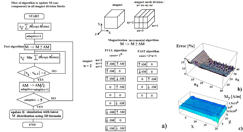
(a) Flow of the algorithm to reconstruct incrementally magnetization in each magnet division of all blocks of Halbach magnet; (b) Survey of error [%] of reconstruction of magnetization with block division n _x −1 − n _z ; (c) reconstruction of magnetization of H-block magnet using 20-1-14 division.

OPEN IN VIEWER

Fig. 5.

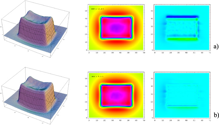
3D plot, contour lines and error (difference to measurements) of magnetic flux distribution above H-block magnet using reconstructed magnetization with a magnet division (n _x − n _y − n _z ) of: (a) 15-1-6, (b) 40-1-40.

Numerical results demonstrate the convergence of the algorithm, when ΔM is usually smaller than 2% of initial magnetization M _y value, to the same magnetization model even with very different initial M _y values but increasing the iterative steps to reach the convergence. The convergence error ϵ was selected as 0.0001. Figure 4c shows a map of the error in the algorithm convergence to the same non-uniform magnetization model, example for 20-1-14, when the division of parallelepiped magnet is n _x −1 − n _z . Starting with the initial M from manufacturer data, the FAST algorithm reconstruction is obtained after a small number of iterations (<100) in short time (<1 hour) for a block magnet unit or a longer time (18 h) for large Halbach magnet (66 blocks) reconstruction (using 24 CPU cores), shown in Table 2. The error is computed as Abs[(B _exp − B _sim )∕Max (B _exp )] to avoid infinite large numbers when magnetization is close to small zero values when is changing its direction from positive to negative values and calibrating the error to the maximum values of magnetizations of each magnet block.

OPEN IN VIEWER

Fig. 6.

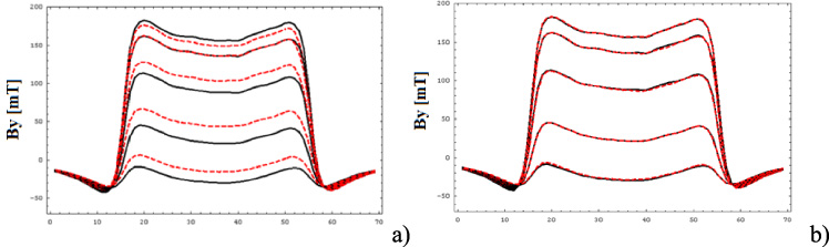
Magnetic flux distribution: measurements (continuous line) vs. simulation (dashed line) using reconstructed magnetization model near edge (line 40 to 44) for a magnet with division n _x − n _y − n _z of (a) 15-1-6, (b) 40-1-40.

A full reconstruction of the H-block unit magnetization model and the computed magnetic flux distribution above magnet surface through theoretical 3D formula is shown in Fig. 5 for two block magnet mesh divisions. The smallest error (5%) in the flux distributions between measurements and simulations when using a single component M _y magnetization model reconstruction is obtained for larger values of n _x (40) and n _z (40) mesh divisions when n _y = 1, as shown in Fig. 4a. The largest error is near the edge of block magnet, (Fig. 6), for the two above reconstructed configurations that minimize the error to minimum for larger n _x and n _z values on all measurements points.

While previously the reconstructed model was focused on single magnet blocks, in Halbach array there are a combination of H and V-blocks with a complicated magnetic flux distribution, measured experimentally and showed in details in Fig. 6. If each block unit is measured separated and each block unit magnetization model is accurately reconstructed with a small error of 5%, than it is possible to compute the Halbach array magnetization model through use of the 3D theoretical model by overlapping the effect of all magnets and computing the flux distribution with the same 5% accuracy.

However, in the next, the authors investigated the performance of Halbach array magnetization reconstruction if no experimental data are available individually from each magnet and instead only one surface measurement (16,587 = 171*97 points, each of them 0.25 mm apart from each other) of Halbach array magnetic field is acquired (see Fig. 7). The reconstructed model, again was limited to reconstruction of only perpendicular M _y magnetization of the each H and V-block unit (Fig. 1a).

By using the manufacturer data of H and V-block magnetization, large errors (26.8%) in the flux density measurements were recorded as presented in Fig. 8a. By using the previous iterative adaptive algorithm, the magnetization model could be reconstructed accurately with a precision of up to 15% for Halbach array as shown in Fig. 8b. However, in the initial reconstruction model a small 0.4 degree no-alignment rotation in the magnet position are visible in the error map. If the magnet model is aligned with experimental measurements through precise alignment the errors in the magnetic flux distributions near magnet edge decreases, while the error on the median line between the two rows of the Halbach array are the one that limits the overall precision of reconstruction to 14 ∼ 15%.

OPEN IN VIEWER

Fig. 7.

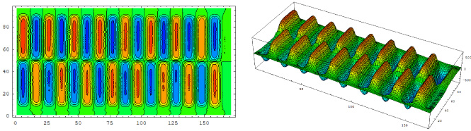
Experimental measurements: contour lines and plot of magnetic flux distribution above Halbach magnet (0.45 mm lift-off).

OPEN IN VIEWER

Fig. 8.

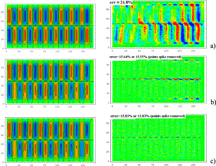
Magnetic flux distribution and error map (difference to measurements) using: (a) initial H and V-block magnetization from manufacturer (b) Reconstructed magnetization model with each H and V-block magnet division: 3-2-9 (c) Reconstructed magnetization model with 0.4 degree rotation adjustment (H and V-block magnet division: 3-1-7).

This is due the strong gradients field between the two magnet rows where magnetic flux distribution decreases very fast from positive to negative values. Other reasons of disagreement are due to the limitation of reconstruction to only one component of the magnetization M _y as well as unevenness of magnet surface or small geometrical variations of gaps (as viewed in Fig. 1a) between magnets, responsible for small spikes in error magnetic field (81 random points in Fig. 8) which after removal decreases the error to 15.55% (no rotation alignment) and 13.83% (with rotation alignment).

It was shown that a “FAST algorithm” to reconstruct magnetization model (based on main component of magnetization M _y inside block magnet), achieves a high performance of error of up to 5% when compared with measured data of magnetic flux distributions outside of block magnet. The accuracy of the non-uniform magnetization model across parallelepiped magnet is controlled accurately by the small adaptive-iterative steps updating the magnetization of each magnet mesh division cells, converging to the same magnetization model, irrespective of the initial magnetization data. The application to the reconstruction of Halbach array magnetization model of the “FAST algorithm” demonstrates the robustness of the method to acquire fast knowledge (hours) of magnetization (M _y ) models for all magnet units in the Halbach array even if only one measurement above the surface of Halbach array magnet is available, but with a lower precision of reconstruction (14 ∼ 15%) due to small geometrical irregularities or unevenness in magnets surface geometries.