Transient magnetic field formulation for solid source conductors

Abstract

The formulation for the azimuthal component of the magnetic vector potential for axisymmetric magnetostatic applications is well known. However for transient magnetic fields with solid source conductors and eddy currents the formulation has to be revised. A variable transformation is introduced to remove the singularity from the numerical scheme. The numerical error cannot accumulate and is put instead to the postprocessing at every time step.

Keywords

Transient magnetic finite element method numerical error

1. Introduction

Axisymmetric models for transient magnetic field simulations play an important role in many electromagnetic applications, for example, magnetic actuators. Exploiting the axial symmetry the problem can be stated as a 2D Finite Element problem in the rz-plane. Here, solid conductors which can carry eddy currents have a prescribed total current while the distribution of the current density is unknown. The current density is composed of the eddy current density and the source current density which is derived from a constant but unknown electric potential. Formulations for axisymmetric models are known, but without the current constraint for solid conductors [1]. First we present the formulation for transient magnetic fields with current constraint for models with infinite length (xy-geometry). Then we derive the formulation for axisymmetric models (rz-geometry) and show that the integration order for the numerical scheme is important to prevent the solver from diverging. Finally, a suitable variable transformation is introduced to increase the stability.

2. Transient magnetic formulation

2.1. Transient magnetic formulation in 3D

The transient magnetic field equation in 3 dimensions can be written as the parabolic differential equation $\begin{eqnarray}\displaystyle {\sigma}\frac{\partial A}{\partial t}+\text{curl}({\nu}∼\text{curl}∼A)=-{\sigma}\text{grad}{\phi} & & \displaystyle\end{eqnarray}$ (1) for the magnetic vector potential A. From the nonphysical quantity A all physical relevant quantities can be calculated. Equation (1) can be derived from the basic Maxwell equations, material relations and neglecting displacement currents ∂D∕∂t which is common in low frequency applications. The material property is given by the magnetic reluctivity 𝜈, the conductors conductivity by σ and 𝜙 the electric scalar potential. Equation (1) is well known and has been investigated by many authors in the past decades. Older publications deal with the derivation of this equations (see [4,5,7,9]). More recent publications deal with solving this equation with various time stepping methods for specific applications as motors and generators (see [2,3,8,10]).

If the problem geometry reveals axial symmetry the problem can be considered as planar solution. Next sections will explain the numerical problems arising from this approach and how to avoid that problem.

Fig. 1.

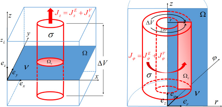
Solid conductor in xy-geometry (left), rz-geometry (right).

2.2. Transient magnetic formulation for solid source conductors in 2D

2.2.1. Infinite conductors – XY -geometry

If the model is extended infinite in one direction and the currents only flow in that direction the 3D model can be represented by a 2D model. Solid source conductors for xy-geometries are discussed in [6]. We refer to that model as xy-geometry. Even no real application reveals infinite extension in one direction many problems can be well approximated by a 2D model as motors and generators. Figure 1 (left) shows a simplified model with one conductor which is extended infinite in z-direction. It can be shown that the magnetic vector potential A = (0,0, A_z)^T only has only one nonzero component A_z. The gradient of the electric scalar potential 𝜙 comes from a voltage drop ΔV which implies an electric field ΔV∕ΔL with ΔL the length of the voltage drop. It is common to use ΔL = 1 m and (1) can be written as $\begin{eqnarray}\displaystyle \text{curl}({\nu}∼\text{curl}(0,0,A_{z})^{T})=\left(-{\sigma}\frac{\partial A_{z}}{\partial t}-{\sigma}{\rm\Delta}V\right)e_{z} & & \displaystyle\end{eqnarray}$ (2) or $\begin{eqnarray}\displaystyle {\sigma}\frac{\partial A_{z}}{\partial t}e_{z}+\text{curl}({\nu}∼\text{curl}(0,0,A_{z})^{T})=-{\sigma}{\rm\Delta}Ve_{z}. & & \displaystyle\end{eqnarray}$ (3) From (3) it can be seen that the overall current density J = (0,0, J_z)^T has only a component J_z in z-direction and consists of the eddy current density $J_{z}^{E}=-{\sigma}∼\partial A_{z}/\partial t$ and the current density $J_{z}^{V}=-{\sigma}∼{\rm\Delta}V$ which comes from the voltage drop along the conductor such that $J_{z}=J_{z}^{E}+J_{z}^{V}$ .

The voltage drop ΔV is usually unknown. Instead the overall current I is known. Hence (3) is augmented by the current constraint equation and the equations $\begin{eqnarray}\displaystyle {\sigma}\frac{\partial A_{z}}{\partial t}e_{z}+\text{curl}({\nu}∼\text{curl}(0,0,A_{z})^{T})=-{\sigma}{\rm\Delta}Ve_{z},\quad \int _{{\Omega}_{c}}\left(-{\sigma}\frac{\partial A_{z}}{\partial t}-{\sigma}{\rm\Delta}V\right)\text{d}x∼\text{d}y=I & & \displaystyle\end{eqnarray}$ (4) have to be solved for the unknowns A_z and ΔV .

2.2.2. Axisymmetric coils – RZ-geometry

If the model shows symmetry with respect to one axis and the currents flow in coils around in azimuthal direction the problem can stated as a 2D problem. Applications like magnetic valves show this symmetry. Figure 1 (right) shows a simplified model with one solid coil. The current J = (0, J_φ,0)^T only has a component in φ-direction. It can be shown that the magnetic vector potential A = (0, A_φ,0)^T has only a nonzero component A_φ in φ-direction. The constant voltage drop ΔV along the circle with radius r yields the electric field ΔV∕(2πr) and (1) can be written with the additional current constraint equation using cylindrical coordinates as $\begin{eqnarray}\displaystyle {\sigma}\frac{\partial A_{{\varphi}}}{\partial t}e_{{\varphi}}+\text{curl}({\nu}∼\text{curl}∼(0,A_{{\varphi}},0)^{T})=-{\sigma}\frac{{\rm\Delta}V}{2{\pi}r}e_{{\varphi}},\quad \int _{{\Omega}_{c}}\left(-{\sigma}\frac{\partial A_{{\varphi}}}{\partial t}-{\sigma}\frac{{\rm\Delta}V}{2{\pi}r}\right)\text{d}r∼\text{d}z=I. & & \displaystyle\end{eqnarray}$ (5) The unknowns are A_φ and ΔV . The overall current density J_φ consists of the eddy current density $J_{{\varphi}}^{E}=-{\sigma}\partial A_{{\varphi}}/\partial t$ and the current density $J_{{\varphi}}^{V}=-{\sigma}{\rm\Delta}V/(2{\pi}r)$ which comes from the constant voltage drop ΔV such that $J_{{\varphi}}=J_{{\varphi}}^{E}+J_{{\varphi}}^{V}$ .

3. Finite element discretization

3.1. Discretization for XY -geometry

The continuous scalar magnetic potential A_z is discretized with classical Lagrangian interpolatory shape functions of any order on a triangular mesh. Let n denote the number of unknowns (dof’s) and N_i = N_i(x, y), i = 1, …, n the shape functions. The weak formulation of (2) and (3) with $A_{z}=\sum _{i=1}^{n}a_{i}N_{i}$ and a: = (a₁, …, a_n)^T yields $\begin{eqnarray}\displaystyle M\frac{\text{d}}{\text{d}t}\left(\begin{array}{@{}c@{}}{\rm\Delta}V\\ a\end{array}\right)+K\left(\begin{array}{@{}c@{}}{\rm\Delta}V\\ a\end{array}\right)=\left(\begin{array}{@{}c@{}}-{\mu}_{0}I\\ 0\end{array}\right) & & \displaystyle\end{eqnarray}$ (6) with the mass element matrix M_e $\begin{eqnarray}\displaystyle M_{e}=\left(\begin{array}{@{}cc@{}}0 & \displaystyle {\mu}_{0}{\sigma}\int _{{\Omega}_{c}}N_{i}\cdot 1∼\text{d}{\Omega}_{S}\\[12.0pt] 0 & \displaystyle {\mu}_{0}{\sigma}\int _{z=z_{0}}^{z_{L}}\int _{{\Omega}}N_{i}\cdot N_{j}\text{d}{\Omega}_{V}\end{array}\right) & & \displaystyle\end{eqnarray}$ (7) and the stiffness element matrix K_e $\begin{eqnarray}\displaystyle K_{e}=\left(\begin{array}{@{}cc@{}}\displaystyle {\mu}_{0}{\sigma}\int _{{\Omega}_{c}}1∼\text{d}{\Omega}_{S} & 0\\[10.0pt] \displaystyle {\mu}_{0}{\sigma}\int _{z=z_{0}}^{z_{L}}\int _{{\Omega}}1\cdot N_{j}∼\text{d}{\Omega}_{V} & \displaystyle {\nu}_{r}\int _{z=z_{0}}^{z_{L}}\int _{{\Omega}}\text{curl}\left(\begin{array}{@{}c@{}}0\\ 0\\ N_{i}\end{array}\right)\cdot \text{curl}\left(\begin{array}{@{}c@{}}0\\ 0\\ N_{j}\end{array}\right)\text{d}{\Omega}_{V}\end{array}\right). & & \displaystyle\end{eqnarray}$ (8) The vacuum permeability is denoted by μ₀ and μ = μ₀μ_r,𝜈_r = 1∕μ_r. The matrices M and K are assembled from the element matrices M_e and K_e by looping over all elements of the mesh respecting the local to global relation of the dof’s. The integrals in the first rows of (7) and (8) are surface integrals d𝛺_S = dx dy over the conductor domain 𝛺_c and in the second row of (7) and (8) are volume integrals d𝛺_V = dx dy dz over the cuboid with bottom area 𝛺 and height z_L − z₀. It is common to set z₀ = 0 m, z_L = 1 m and hence the mass and stiffness element matrix are $\begin{eqnarray}\displaystyle \hspace{-12.0pt}M_{e}=\left(\begin{array}{@{}cc@{}}0 & \displaystyle {\mu}_{0}{\sigma}\int _{{\Omega}_{c}}N_{i}\cdot 1∼\text{d}{\Omega}_{S}\\[10.0pt] 0 & \displaystyle {\mu}_{0}{\sigma}\int _{{\Omega}}N_{i}\cdot N_{j}∼\text{d}{\Omega}\end{array}\right),\quad K_{e}=\left(\begin{array}{@{}cc@{}}\displaystyle {\mu}_{0}{\sigma}\int _{{\Omega}_{c}}1∼\text{d}{\Omega}_{S} & 0\\ \displaystyle {\mu}_{0}{\sigma}\int _{{\Omega}}1\cdot N_{j}∼\text{d}{\Omega} & \displaystyle {\nu}_{r}\int _{{\Omega}}\text{curl}\left(\begin{array}{@{}c@{}}0\\ 0\\ N_{i}\end{array}\right)\cdot \text{curl}\left(\begin{array}{@{}c@{}}0\\ 0\\ N_{j}\end{array}\right)\text{d}{\Omega}\end{array}\right). & & \displaystyle\end{eqnarray}$ (9) The integration domain in the second rows of (9) is the 2D domain 𝛺. The curl of (0,0, N_i)^T is given by $\begin{eqnarray}\displaystyle \text{curl}\left(\begin{array}{@{}c@{}}0\\ 0\\ N_{i}\end{array}\right)=\text{curl}(N_{i}e_{z})=\frac{\partial N_{i}}{\partial y}e_{x}-\frac{\partial N_{i}}{\partial x}e_{y} & & \displaystyle\end{eqnarray}$ (10) where e_x, e_y and e_z denote the unit vectors in the cartesian coordinate system. Applying standard time integration methods with step size Δt to (6) as implicit Runge–Kutta methods a linear system with coefficient matrix M∕Δt + K can be derived. After rescaling this matrix can be made symmetric which is suitable for linear solvers. Once the unknowns a and ΔV are known in every time step the magnetic flux density can be derived as $\begin{eqnarray}\displaystyle B=\text{curl}∼A=\mathop{\sum }_{i=1}^{n}a_{i}\left(\frac{\partial N_{i}}{\partial y}-\frac{\partial N_{i}}{\partial x}\right). & & \displaystyle\end{eqnarray}$ (11)

3.2. Discretization for RZ-geometry

The weak formulation of (5) which is obtained by multiplying the first equation of (5) with a suitable test function and integrating over the cylinder volume (Fig. 1, right: blue cylinder) is to be discretized with $A_{{\varphi}}=\sum _{i=1}^{n}a_{i}N_{i}$ , N_i = N_i(r, z) and a: = (a₁, …, a_n)^T and the test function N_j = N_j(r, z) results in $\begin{eqnarray}\displaystyle \hspace{-18.0pt}M\frac{\text{d}}{\text{d}t}\left(\begin{array}{@{}c@{}}{\rm\Delta}V/(2{\pi}r)\\ a\end{array}\right)+K\left(\begin{array}{@{}c@{}}{\rm\Delta}V/(2{\pi}r)\\ a\end{array}\right)=\left(\begin{array}{@{}c@{}}-{\mu}_{0}I\\ 0\end{array}\right). & & \displaystyle\end{eqnarray}$ (12) The element matrices M_e and K_e are $\begin{eqnarray}\displaystyle \hspace{-18.0pt}\begin{array}{@{}c@{}}\displaystyle M_{e}=\left(\begin{array}{@{}cc@{}}0 & \displaystyle {\mu}_{0}{\sigma}\int _{{\Omega}_{c}}N_{i}\cdot 1∼\text{d}{\Omega}_{S}\\[12.0pt] 0 & \displaystyle {\mu}_{0}{\sigma}\int _{{\Omega}}N_{i}\cdot N_{j}∼\text{d}{\Omega}_{V}\end{array}\right),\quad \displaystyle K_{e}=\left(\begin{array}{@{}cc@{}}\displaystyle {\mu}_{0}{\sigma}\int _{{\Omega}_{c}}1∼\text{d}{\Omega}_{S} & 0\\[10.0pt] \displaystyle {\mu}_{0}{\sigma}\int _{{\Omega}}1\cdot N_{j}∼\text{d}{\Omega}_{V} & \displaystyle {\nu}_{r}\int _{{\Omega}}∼\text{curl}∼\left(\begin{array}{@{}c@{}}0\\ N_{i}\\ 0\end{array}\right)\cdot \text{curl}\left(\begin{array}{@{}c@{}}0\\ N_{j}\\ 0\end{array}\right)\text{d}{\Omega}_{V}\end{array}\right)\end{array} & & \displaystyle\end{eqnarray}$ (13) with d𝛺_S = dr dz and d𝛺_V = 2πr dr dz. The evaluation of K_e is critical since the curl of N_ie_φ can be written $\begin{eqnarray}\displaystyle \text{curl}∼N_{i}e_{i}=-\frac{\partial N_{i}}{\partial z}e_{r}+\frac{1}{r}\frac{\partial }{\partial r}(r\cdot N_{i})e_{z} & & \displaystyle\end{eqnarray}$ (14) and contains a singularity at r = 0. It is obvious that this could be the source of numerical problems.

4. Variable transformation

The singularity in ((14)) can be removed by using the variable transformation $\begin{eqnarray}\displaystyle A_{{\varphi}}^{\ast }:=\frac{A_{{\varphi}}}{r},\quad N_{i}^{\ast }:=\frac{N_{i}}{r},\quad N_{j}^{\ast }:=\frac{N_{j}}{r}. & & \displaystyle\end{eqnarray}$ (15) The (4,4)-entry is transformed as $\begin{eqnarray}\displaystyle \int _{{\Omega}}\text{curl}(N_{i}e_{{\varphi}})\cdot \text{curl}(N_{j}e_{{\varphi}})∼\text{d}{\Omega}_{V} & = & \displaystyle 2{\pi}\int _{{\Omega}}r^{3}\left(\frac{\partial N_{i}^{\ast }}{\partial r}\cdot \frac{\partial N_{j}^{\ast }}{\partial r}+\frac{\partial N_{i}^{\ast }}{\partial z}\cdot \frac{\partial N_{j}^{\ast }}{\partial z}\right)\text{d}r∼\text{d}z\nonumber\\ \displaystyle \text{} & \text{} & \displaystyle +∼2{\pi}\int _{{\Omega}}r^{2}\left(2N_{i}^{\ast }\cdot \frac{\partial N_{j}^{\ast }}{\partial r}+2N_{j}\cdot \frac{\partial N_{i}^{\ast }}{\partial r}\right)\text{d}r∼\text{d}z\nonumber\\ \displaystyle \text{} & \text{} & \displaystyle +∼2{\pi}\int _{{\Omega}}4r(N_{i}^{\ast }\cdot N_{j}^{\ast })∼\text{d}r∼\text{d}z.\end{eqnarray}$ (16) Hence (15) no longer contains the singularity. However its has not been removed completely. At every time step the back transformation has to be done for calculating the magnetic flux density B: = curl A. But the singularity has been removed from the time stepping scheme such that errors cannot accumulate over the time.

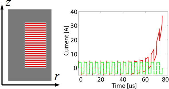
5. Wave transformer

In Fig. 2 the rz-geometry of a cylindrical wave transformer with several conductors in an iron core is shown. In one conductor, which is the source conductor, the current I is prescribed as a rectangular signal which is shown in Fig. 2 as green dashed curve and can be recalculated from $\begin{eqnarray}\displaystyle I=\int _{{\Omega}_{c}}\left(-{\sigma}\frac{\partial A_{{\varphi}}}{\partial t}-{\sigma}∼\frac{{\rm\Delta}V}{2{\pi}r}\right)\text{d}r∼\text{d}z & & \displaystyle\end{eqnarray}$ (17) according to (17). Figure 2 (right) shows the source current which is calculated by (17) and using implicit Euler for the time stepping. The solid red curve is obtained from the standard formulas ((12)) and ((13)) containing the singularity and the green curve shows the curve using the variable transformation. Of course, the problems arising from the singularity might not be dominant in other examples and no variable transformation might be needed. However this example should show that divergence could happen and how to avoid it.

Fig. 2.

Wave transformer in rz-geometry (left), current curves (right).

6. Conclusion

The numerical solution of the transient magnetic field equation which is solved with 2D finite elements for axisymmetric models can become instable due to a singularity. Small errors which are made when evaluating the stiffness matrix accumulate over the time and causes the solver to diverge. A variable transformation removes that singularity and puts it instead to the in each time step postprocessing.

References

Asche

and Sattler

Ph.K.

, Numerical calculation of the dynamic behaviour of electromagnetic actuators, IEEE Transactions on Magnetics26(2) (1990), 979–982.

Clemens

Lang

Teleaga

and Wimmer

, Transient 3D magnetic field simulations with combined space and time mesh adaptivity for lowest order whitney finite element formulations, IET Science, Measurement and Technology3(6) (2009), 377–383.

Clemens

Wilke

and Weiland

, Linear-implicit time integration schemes for error-controlled transient nonlinear magnetic field simulations, IEEE Transactions on Magnetics39(3) (2003), 1175–1178.

Emson

C.R.I.

and Simkin

, An optimal method for 3-D eddy currents, IEEE Transactions on Magnetics19(6) (1983), 2450–2452.

Emson

C.R.I.

and Trowbridge

C.W.

, Transient 3D eddy currents using modified magnetic vector potentials and magnetic scalar potentials, IEEE Transactions on Magnetics24(1) (1988), 86–89.

W.N.

Zhou

Lin

Stanton

and Cendes

Z.J.

, Modeling of solid conductors in two-dimensional transient finite-element analysis and its application to electric machines, IEEE Transactions on Magnetics40(2) (2004), 426–434.

Konrad

and Silvester

, Triangular finite elements for the generalized bessel equation of order m, International Journal for Numerical Methods in Engineering7 (1973), 43–55.

H.L.

S.L.

and Fu

W.N.

, Application of multi-stage diagonally-implicit Runge–Kutta algorithm to transient magnetic field computation using finite element method, IEEE Transactions on Magnetics48(2) (2012), 279–282.

Weiss

and Cendes

, Efficient finite element solution of multipath eddy current problems, IEEE Transactions on Magnetics18(6) (1982), 1710–1712.

10.

Wimmer

Steinmetz

and Clemens

, Reuse, recycle, reduce (3R) - strategies for the calculation of transient magnetic fields, Applied Numerical Mathematics59 (2009), 830–844.