A tidal energy harvesting system in point of view of the robotic notation

Abstract

To represent energy gathered in energy harvester, it is necessary to simulate movement of the energy harvester parts. The aim of this article is to present a new way to simulate movement of energy harvester in point of view of robotic approach. The power buoy is one of the best examples to show potentiality of modelling such mechanism as robotic chain. In the article two ways of buoy’s motion are presented. As a result it occurs that it is possible to use robots kinematic chain theory to present kinematic chain of energy harvesting system.

Keywords

Energy harvesting homogenous transformation wave energy harvester buoy movement

1. Introduction

Nowadays energy harvesting is one of the main topics due to environment pollution caused by fossil fuels and also high cost of fuels. The harvested energy is kinetic energy [1], therefore it is necessary to calculate the movement of the energy carrier of the energy harvester. To simulate this movement, by formulating force and torque equations, Newton’s laws or Lagrange’s equation can be used [2,3]. Kinematic chain of energy harvester is similar to kinematic chain of a robot, due this fact it is possible to use theory of formulation of robot movement equations to formulate equation of harvester movement. These are Euler–Lagrange’s equations and they are using generalized variables that are describing movement of the kinematic chain joints [4]. This method can be used for different types of energy harvesters. In the paper homogenous transformation and Euler–Lagrange’s equation formulated from transformations and used for harvester’s movement simulation are presented.

This method can be used to describe behaviour of object related to robotics and to determine exact position of the end of actuators, for example for 3D printers systems modelling [5], hard disk drive head positioning, VCM motor as a drive of actuator arm modelling [6–8]. Mathematical representation of the positioning can be used for modelling in Simulink/Matlab [7–9]. If inertia matrix is more complicated, method of inversion of block matrix can be used to resolve the dynamic equations, as it is described in [7,9].

Wave energy seems to be a good alternative for fossil fuels energy, because 70% of the planet’s surface are covered by oceans [10]. Tidal energy is the most reliable and predictable source of renewable energy because the time in which waves arrive to the coast is a result of gravitational attraction of the moon and the sun [1,11]. Tidal energy harvesters have to be located near a coast, where waves are more efficient. The cost of energy transmission for that location is lower than for buoys far away from a coast but harvesters need to be located away from ports because of safety requirements and beaches because of landscape pollution.

Wave energy harvesters can be divided into different types e.g. oscillating water column [12], tapered channel, power buoy [10,11,13], Salterduck (nodding duck) [14]. As follow in [14] power buoy plant can harvest more energy than other harvesters using the same area. For that the types of movement of power buoy – wave energy harvester were analysed. Energy harvested from the buoy movements is mostly harvested from the heaving movements but also from the pitching movement.

2. Powerbuoy energy harvester analysis

2.1. Powerbuoy model

As a power buoy, different kind of buoys can be used, i.e. buoys on platform with instruments to register oceanographic and meteorological data [13], buoys that are used to lead the way or only to harvest energy. Using buoys that are already on the ocean to harvest energy is economic and it can be used also to provide energy to electronic instruments on buoy platform.

Power buoys should be composed from floating buoy, anchor, chain, rope, generator and spring that accumulate energy [15]. Generator can be linear or rotational and it determine efficiency of harvester and the movement conversion type. Model of the buoy is shown in Fig. 1.

Fig. 1.

Power buoy model.

2.2. Powerbuoy movement

The buoy floats on the ocean. Wave movement moves the buoy and that movement is changed into electrical energy using converters to harvest energy from waves. Buoy moves up and down-heaves but also pitches. Heaving movement is transmitted to either linear or rotational generator. Rotational generator requires movement conversion system but it is smaller and more efficient than a linear one [3,16]. In this paper only movement of the buoy is considered, so only generator influence on the buoys mass should be considered. Movement of the buoy can be described by Newton’s law like in all mechanical systems. It is called force balance equation and torque balance equation.

Fig. 2.

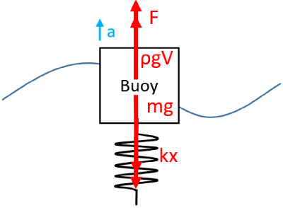
Forces acting on the buoy and acceleration of the buoy.

For the description of linear movement, equation of force (1) can be used. F is force that is acting on the buoy with mass m and linear acceleration a of the buoy. The force of gravity and buoyancy are acting on the buoy, so they should be written in equation. The buoy accumulates its energy in energy accumulation spring so spring force is also used in force equation. Gravitation acceleration is g, spring constant is k, up and down movement is x, volume of the buoy is V and density of the oceanic water is 𝜌. Sign of the force components depends on direction of the force. If external force is not acting on buoy then F is equal to 0. Schema of forces acting on the buoy and acceleration of the buoy, according to which force balance equation is written, is shown in Fig. 2. Localisation of the energy accumulation spring does not matter because force of the spring will be always opposite to the external force which is acting on buoy. Acceleration of the buoy is sum of total forces acting on buoy. $\begin{eqnarray}\displaystyle F=ma+mg+kx-{\rho}gV. & & \displaystyle\end{eqnarray}$ (1)

For the description of buoy’s heaving and pitching movement, equations of torque and force (2), (3) can be used. ω is rotational speed, ϵ is rotational acceleration, R is radius of buoy’s rotation, v is linear speed of the buoy. In torque equation Coriolis force should be considered. Gravity force, buoyancy force and spring force are acting on the mass centre so they should not be written in torque equation because radius on which they are acting is equal to 0. From the centripetal acceleration of buoy only tangential acceleration is considered in torque equation. If external torque is not acting on buoy then τ is equal to 0. Schema of forces and torque acting on the buoy and accelerations of the buoy, according to which force and torque balance equations are written, is shown in Fig. 3. Centripetal acceleration of buoy are written on schema as a_cn and a_cτ, first one is normal acceleration and second tangential. Normal acceleration is result of multiplying square of rotational velocity and radius of force acting on buoy and tangential acceleration is result of multiplying rotational acceleration and radius of force acting on buoy. $\begin{eqnarray}\displaystyle \text{} & \text{} & \displaystyle F=ma-m{\omega}^{2}R+mg+kx-{\rho}gV\end{eqnarray}$ (2) $\begin{eqnarray}\displaystyle \text{} & \text{} & \displaystyle {\tau}=m{\varepsilon}R^{2}+I{\varepsilon}+2mv∼{\omega}R.\end{eqnarray}$ (3)

Description of buoy’s movement with more degrees of freedom is more complicated using only force and torque balance equation. The idea was to simplify finding the solution of movement description.

Fig. 3.

Forces and torque acting on the buoy and acceleration of the buoy.

Fig. 4.

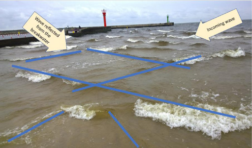
Waves movement near the shore.

3. Robotic approach to powerbuoy modeling

Buoy can heave, pitch and rotate, so it is possible to create kinematic chain of robot that includes that movements. Movement of the buoy is caused by waves movement in different directions, for example wave reflection from the breakwater and incoming tidal wave (Fig. 4). As a result of external forces influence, such as wind or gravitational forces, wave is modulated. That also lead to variability in buoy movement. Number of degrees of freedom depends of incoming waves behavior [17].

In the paper two of possible kinematic chains are considered: first 1-DoF with linear movement (Fig. 5a) and the second with 2-DoF with linear and pitching movements (Fig. 5b). The more degrees of freedom the kinematic chain has the more accurate the simulation of buoy’s movement is but it is necessary to take into account all possible movements and not to overrate the number of joints.

Fig. 5.

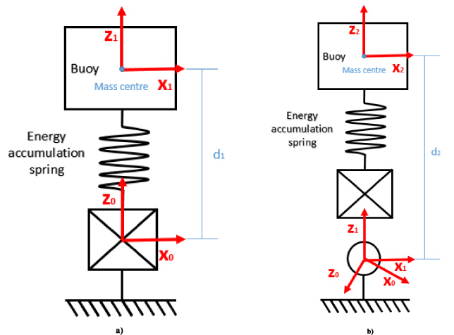
1-DoF kinematic chain of buoy movement (a), 2-DoF kinematic chain of buoy movement (b).

3.1. Heaving movement system

Buoy moves up and down which means prismatic joint should be used in kinematic chain. That kinematic chain has one degree of freedom (1-DoF). Kinematic chain of heaving buoy with energy accumulation spring is shown in Fig. 5a.

To describe forces that are acting on buoy Denavite–Hartenberg notation is used. It is shown in Table 1, where: i is ordinal number of link, a_i is distance between axis z_i and z_i−1, 𝛼_i is angle between axis z_i and z_i−1, d_i is distance between axis x_i and x_i−1 and 𝛩_i is angle between axis x_i and x_i−1, symbol * above letter means that it is variable.

Table 1
Kinematic parameters for heaving movement of buoy

i a _i 𝛼_i d _i 𝛩_i

1 0 0 $d_{1}^{\ast }$ 0

i	a _i	𝛼_i	d _i	𝛩_i
1	0	0	$d_{1}^{\ast }$	0

From Denavite–Hartenberg notation homogenous transformation and then force equation can be formulated. Homogenous transformation H is obtained from rotation and translation about the x and z axis (4). Homogenous transformation for whole kinematic chain is product of homogenous transformations A for each transformation from frame i to frame i − 1 (5). $\begin{eqnarray}\displaystyle \text{} & \text{} & \displaystyle H=\left[\begin{array}{@{}cc@{}}R & d\\ 0 & 1\end{array}\right]=\left[\begin{array}{@{}cc@{}}\mathit{rotation} & \mathit{transformation}\\ \mathit{perspective } & \mathit{ scale }∼\mathit{ factor }\end{array}\right]\end{eqnarray}$ (4) $\begin{eqnarray}\displaystyle \text{} & \text{} & \displaystyle A_{i}=Rot_{z_{i}{\theta}_{i}}\mathit{Trans}_{z_{i}d_{i}}\mathit{Trans}_{x_{i}a_{i}}Rot_{x_{i}{\alpha}_{i}}=\left[\begin{array}{@{}cccc@{}}c{\theta}_{i} & -s{\theta}_{i}c{\alpha}_{i} & s{\theta}_{i}s{\alpha}_{i} & a_{i}c{\theta}_{i}\\ s{\theta}_{i} & c{\theta}_{i}c{\alpha}_{i} & -c{\theta}_{i}s{\alpha}_{i} & a_{i}s{\theta}_{i}\\ 0 & s{\alpha}_{i} & c{\alpha}_{i} & d_{i}\\ 0 & 0 & 0 & 1\end{array}\right].\end{eqnarray}$ (5)

First, from coordinates of the axis and the base, Jacobians of linear and rotational speed can be obtained. Jacobian matrix contains Jacobian of linear speed J_vi and Jacobian of rotational speed J_ωi. For prismatic joint i Jacobian is shown in (6) and it depends on z axis of i − 1 joint. For rotational joint Jacobian matrix is shown in (7) and it depends on z axis of i − 1 joint and on the centre of last joint minus coordinates of the centre of the i − 1 joint. $\begin{eqnarray}\displaystyle \text{} & \text{} & \displaystyle J_{i}=\left[\begin{array}{@{}c@{}}J_{vi}\\ J_{{\omega}i}\end{array}\right]=\left[\begin{array}{@{}c@{}}z_{i-1}\\ 0\end{array}\right]\end{eqnarray}$ (6) $\begin{eqnarray}\displaystyle \text{} & \text{} & \displaystyle J_{i}=\left[\begin{array}{@{}c@{}}J_{vi}\\ J_{{\omega}i}\end{array}\right]=\left[\begin{array}{@{}c@{}}z_{i-1}\times (o_{n}-o_{i-1})\\ z_{i-1}\end{array}\right].\end{eqnarray}$ (7)

For prismatic joint of the 1-DoF buoy kinematic chain Jacobian of linear speed is equal to coordinates of the z axis that means [0;0;1] and Jacobian of rotational speed is equal to zero.

Linear and rotational kinetic energy can be calculated using Jacobians (8). Kinetic energy depends on Jacobians of linear and rotational speed for all joints, mass and inertia of these joints and on differential of vector of generalized displacement. Matrix R_i is rotation matrix that enforces formulation of rotational speed coordinates depending on link i coordinates. I_i is an inertia matrix of link i, evaluated around a coordinate parallel to frame i. Product of mass of the first joint, mass of the buoy, and square of Jacobian of linear speed for first joint is component of linear kinetic energy. Product of inertia of the first joint, of the buoy, and square of Jacobian of rotational speed for first joint is component of rotational kinetic energy. $\begin{eqnarray}\displaystyle E_{k}=\frac{1}{2}\dot{q}^{T}\mathop{\sum }_{i=1}^{n}[m_{i}{J_{v_{ci}}(q)}^{T}J_{v_{ci}}(q)+{J_{{\omega}_{ci}}(q)}^{T}{R_{i}(q)I_{i}{R_{i}(q)}^{T}J}_{{\omega}_{ci}}(q)]\dot{q}=\frac{1}{2}\dot{q}^{T}D(q)\dot{q}. & & \displaystyle\end{eqnarray}$ (8)

From components of kinetic energy inertia matrix D and Christoffel’s matrix C can be calculated. Matrix D is sum of the components of kinetic energy such as Jacobians of linear and rotational speed for all joints, mass and inertia of these joints. For the heaving movement of the buoy it means that D is equal to mass of the buoy m. Matrix C is equal to zero, because elements of matrix D are independent from generalized variable d₁, it has constant components so differential of matrix D is equal to zero.

Buoyancy of the water and gravity of the earth are components of potential energy. The energy accumulation spring should be considered too, as an element attached to the buoy. Energy of that spring is also potential energy. Potential energy V_e is shown in (9). $\begin{eqnarray}\displaystyle V_{e}=m_{1}gd_{1}-{\rho}gVd_{1}+\frac{1}{2}kd_{1}^{2}. & & \displaystyle\end{eqnarray}$ (9)

Force F_v from potential energy is equal to differential of potential energy by generalized variable d₁.

Equation (10) describes force that is acting on the buoy. It is a result of the movement of end of manipulator. Equation of the force is formulated from Euler–Lagrange equations [4]. Movement d₁ is a prismatic joint position, so it is a heaving movement of the buoy. Generalized variable d₁ is movement of the buoy in z-axis direction. Mass m₁ is the only mass and it is the mass of the buoy so it is written as constant m. $\begin{eqnarray}\displaystyle F=D\ddot{d}_{1}+C{\dot{d}}_{1}+F_{v}=m\ddot{d}_{1}+mg-{\rho}gV+kd_{1}. & & \displaystyle\end{eqnarray}$ (10)

3.2. Heaving and pitching movement system

Kinematic chain for buoy heaving and pitching is 2-DoF and has prismatic joint and revolute joint. Kinematic chain of heaving and pitching buoy with energy accumulation spring is shown in Fig. 5b. That kinematic chain with more accuracy approximate movement of the buoy on the ocean waves, because pitching movement of the buoy has influence on heaving movement of the buoy and vice versa.

The same notation as in 1-DoF kinematic chain is used to create matrix of homogenous transformation and then to formulate equation of heaving and rotating movement. Denavite–Hartenberg notation for that chain with two variables is shown in Table 2.

Table 2
Kinematic parameters for heaving and pitching movement of buoy

I a _i 𝛼_i d _i 𝛩_i

1 0 π∕2 0 ${\Theta}_{1}^{\ast }$

2 0 0 $d_{2}^{\ast }$ 0

I	a _i	𝛼_i	d _i	𝛩_i
1	0	π∕2	0	${\Theta}_{1}^{\ast }$
2	0	0	$d_{2}^{\ast }$	0

Homogenous transformation for whole kinematic chain $T_{0}^{2}$ is product of homogenous transformation for first joint A1 (first row of the Table 2) and homogenous transformation for second joint A2 (second row of the Table 2), which are formulated from Denavite–Hartenberg notation as it was described in chapter III A.

To calculate Jacobians it is necessary to use Denavite–Hartenberg notation for the mass centre, that means only for mass centre of the buoy. Denavite–Hartenberg notation for the mass centre is shown in Table 3. Formulation of homogenous transformation is similar to homogenous transformation formulated from Table 2.

Table 3

Kinematic parameters for the mass centre for heaving and pitching movement of buoy

I	a _i	𝛼_i	d _i	𝛩_i
1	0	0	0	${\Theta}_{1}^{\ast }$
2	0	0	$d_{c2}^{\ast }$	0

To calculate force and torque every mass centre, here only one, and every joint should be considered. For revolute joint Jacobian of linear speed is product of axis z coordinates of the previous link and coordinates of the centre of first joint minus coordinates of the centre of the base, it means vector [0;0;0]. Jacobian of rotational speed is axis of the previous link, it means vector [0;0;1].

The Jacobian of speed for first joint is matrix with elements of linear and rotational speed.

Second joint is linear so Jacobian of linear speed is equal to coordinates of the z axis of previous link [sθ₁; −cθ₁;0] and Jacobian of rotational speed is equal to 0. It is necessary to consider also the first joint. Jacobian of linear speed is dependent on centre of second joint [d_c2sθ₁; −d_c2cθ₁;0] and it is calculated as product of axis z coordinates of the previous link and coordinates of the centre of second joint minus coordinates of the centre of the base [d_c2cθ₁; d_c2sθ₁;0] and Jacobian of rotational speed is coordinates of z axis of the base [0;0;1].

The Jacobian of speed for second joint is matrix with elements of linear and rotational speed for the first joint with its dependence on centre O_c2 and second joint.

Components of linear and rotational kinetic energy can be calculated using Jacobians.

Linear kinetic energy component for first joint is product of mass of the first joint and square of first 3 rows of the Jacobian for the first joint. Mass of the first joint is equal to zero, so linear kinetic energy component for first joint is equal to zero. Linear kinetic energy component for second joint is product of mass of the second joint and square of first 3 rows of the Jacobian for the second joint. Mass of the second joint m₂ is mass of the buoy. As the result of linear kinetic energy components are two matrixes 2 × 2.

Rotational kinetic energy component for first joint is product of inertia of the first joint and square of last 3 rows of the Jacobian for the first joint. Inertia of the first joint I₁ is inertia of the buoy. Rotational kinetic energy component for second joint is product of inertia of the second joint and square of last 3 rows of the Jacobian for the second joint. Inertia of the second joint is equal to zero. As the result of rotational kinetic energy components are two matrixes 2 × 2.

From components of kinetic energy inertia matrix D can be formulated as a sum of kinetic energy components (11). $\begin{eqnarray}\displaystyle D=\left[\begin{array}{@{}cc@{}}m_{2}d_{c2}+I_{1} & 0\\ 0 & m_{2}\end{array}\right]. & & \displaystyle\end{eqnarray}$ (11)

Elements of Christoffel’s matrix C (12) c₁₁, c₁₂, c₂₁, c₂₂ can be calculated from elements of D matrix: d₁₁, d₁₂, d₂₁, d₂₂. They are differential of this components by generalized variables θ₁ and d₂ and then sum of this differentials. $\begin{eqnarray}\displaystyle C=\left[\begin{array}{@{}cc@{}}m_{2}d_{c2}{\dot{z}}_{2} & m_{2}d_{c2}\dot{{\theta}}_{1}\\ -m_{2}d_{c2}\dot{{\theta}}_{1} & 0\end{array}\right]. & & \displaystyle\end{eqnarray}$ (12)

Components of potential energy are buoyancy of the water and gravity of the earth. Energy of the energy accumulation spring attached to the buoy is also written in potential energy equation that is similar to (9) but generalized variable d₁ is change to d₂. Force F_v is differential of V_e by d₂.

Equations of force and torque that are acting on the buoy can be written in matrix form (13) using Euler–Lagrange’s equations [11]. They are result of the movement of the robot’s manipulator’s end. θ₁ is angle of rotation, d₂ is change of the prismatic joint position. $\begin{eqnarray}\displaystyle \left[\begin{array}{@{}c@{}}{\tau}\\ F\end{array}\right]=D\left[\begin{array}{@{}c@{}}\ddot{{\theta}}\\ \ddot{z}\end{array}\right]+C\left[\begin{array}{@{}c@{}}\dot{{\theta}}\\ {\dot{z}}\end{array}\right]+\left[\begin{array}{@{}c@{}}0\\ F_{v}\end{array}\right]. & & \displaystyle\end{eqnarray}$ (13)

Multiplying components of matrixes force equation (14) and torque equation (15) are formulated. Mass m₂ is mass of the buoy and it is the only mass in equations so it can be written as constant m. Generalized variable d_c2 and variable z are the same as generalized variable d₂. Variable θ is the same as variable θ₁. $\begin{eqnarray}\displaystyle \text{} & \text{} & \displaystyle F=m\ddot{d}_{2}-m\dot{{\theta}}_{1}^{2}d_{2}+mg-{\rho}gV+kd_{2}\end{eqnarray}$ (14) $\begin{eqnarray}\displaystyle \text{} & \text{} & \displaystyle {\tau}=md_{2}^{2}\ddot{{\theta}}_{1}+I_{1}\ddot{{\theta}}_{1}+2md_{2}\dot{{\theta}}_{1}{\dot{d}}_{2}.\end{eqnarray}$ (15)

4. Simulation

Energy harvested from the buoy’s movement and movement of the buoy can be simulated in two models in Simulink. The concept of 1-DoF model is shown in Fig. 6 and of 2-DoF in Fig. 7.

Fig. 6.

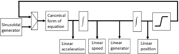
Concept of model of 1-DoF buoy movement.

Fig. 7.

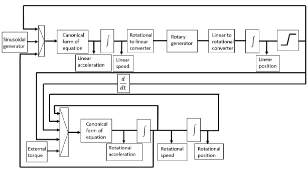
Concept of model of 2-DoF buoy movement.

To obtain the plot of position or velocity of the buoy over time it is necessary to simulate waves movement. Sea waves are irregular but to make analysis easier it is assumed that waves are sinusoidal. According to Douglass Sea Scale the average height of sea wave is from 1.25 m to 2.5 m height and low height is from 0.1 m to 0.5 m. It is assumed that simulated waves have heights H: 0.25 m, 1.75 m or 2.5 m. Waves caused by wind and gravity have a period from 1 s to 20 s. It is assumed that simulated waves period T is equal to 1.5 s or 3.5 s. Wave with period T equal 3.5 s and height H equal 1.75 m was simulated in [18].

Linear position of the buoy is limited by spring elasticity. In 1-DoF model the canonical form of Eq. (10) was used. In 2-DoF model the canonical form of equation after sinusoidal generator – wave force is the canonical form of Eq. (14) and after external torque is the canonical form of Eq. (15).

The electrical generator is used to generate electrical power from movement of the buoy. If a generator is rotary it is necessary to use linear to rotational converter.

The wave force is simplified to sinus generated by the generator multiply by wave energy E_w (16) as an amplitude [14]. $\begin{eqnarray}\displaystyle E_{w}=\frac{{\rho}H^{2}g}{8}. & & \displaystyle\end{eqnarray}$ (16)

The static buoyancy force and gravitational force are equal, the dynamic buoyancy of the buoy is a part of wave force.

Mass of the buoy m is 250 kg, elasticity coefficient k is 10 kN, oceanic water density 𝜌 is 1030 kg/m³, radius of the buoy r is 2.5 m high of the buoy h is 0.5 m, the buoy has a cylindrical shape, these parameters are theoretical and can be applied to the sea buoy or ocean buoy, not to the laboratory one, which should be smaller [18]. Spring maximum length is 2 m. In Figs 8, 9, 10 the movement of the buoy for 1-DoF and for 2-DoF models for wave period T equals 1.5 s (left side) and 3.5 s (right side) and wave height H equals respectively 0.25 m, 1.75 m and 2 m, is shown.

Fig. 8.

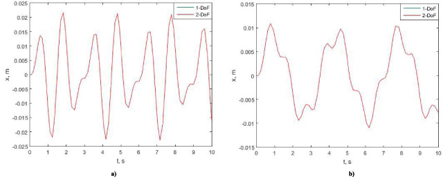
Simulated movement of the buoy for 1-DoF and 2-DoF system for 0.25 m wave height for (a) 1.5 s wave period, (b) 3.5 s wave period.

Fig. 9.

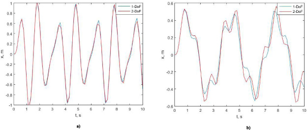
Simulated movement of the buoy for 1-DoF and 2-DoF system for 1.75 m wave height for (a) 1.5 s wave period, (b) 3.5 s wave period.

Fig. 10.

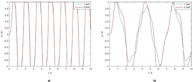
Simulated movement of the buoy for 1-DoF and 2-DoF system for 2.5 m wave height for (a) 1.5 s wave period, (b) 3.5 s wave period.

Using linear generator with induction coil with parameters like in [19], in which linear generator for Powerbuoy is described, the expected power is calculated. Parameters of linear generator working according to Faraday law are theoretical. Resistance and inductance of coil are equal respectively R = 0.045 Ω, L = 0.48 H, length of coil l = 0.4823 m, coil turns N = 200 and resistance of load, calculated from wave frequency and resistance and inductance of the coil, that means R_l = 1.317 Ω for T = 3.5 s and R_l = 2.4606 Ω for T = 1.5 s. Flux density is approximated as negative parabola with offset 0.75 T. Mean values of the expected power are shown in Table 4.

Table 4

Mean values of the expected power

Height H [m]	Period T [s]	Power for 1-DoF P [W]	Power for 2-DoF P [W]
0.25	1.5	2.7305	2.7306
1.75	1.5	6.396 × 10³	6.199 × 10³
2.5	1.5	18.509 × 10³	18.450 × 10³
0.25	3.5	0.232	0.232
1.75	3.5	538.549	671.275
2.5	3.5	2.102 × 10³	3.512 × 10³

The energy harvested from one buoy could be used as power for meteorological station. Buoy farm energy could be used as a support in the energy grid, coastal lightning or harbor lightning. Power is dependent on height and period of the wave so it has to be converted to be more stable. It can be seen that simulated power is dependend on degrees of freedom of the model when a period of wave is lower or for higher waves.

5. Conclusion

It is possible to describe the movement of the energy harvester using kinematic chain of robots with joints responding to possible movement. Comparing Euler–Lagrange equation to force and torque balance equations it can be deduced that these two methods are equivalent. Equation (1) is similar to (10). Equations (2) and (3) are similar to (14) and (15). It is necessary to take into account that $\ddot{{\theta}}_{1}$ is equal to ϵ, $\dot{{\theta}}_{1}$ is equal to ω, d₂ is equal to x, ${\dot{d}}_{2}$ is equal to v and $\ddot{d}_{2}$ is equal to a. For simpler systems it is better to use force and torque balance equations, because there is less calculation, but in more complicated systems it is difficult to formulate balance equations. Euler–Lagrange equation can be used also for validation of obtained equation in simpler mechanisms. More complicated system, with more degrees of freedom, can be simulated using kinematic chain of manipulator to improve and ease simulation of energy harvester movement.

References

Krithika

Chittal

Nandhini

Design and fabrication of tidal energy harvester, in: 2017 IEEE International Conference on Power, Control, Signals and Instrumentation Engineering (ICPCSI), India, 2017, pp. 25102–25107.

Zhao

Sun

and Sheng

, A concept design of a small ocean vehicle with flap-foils to harvest wave energy, in: OCEANS 2016 – Shanghai, China, 2016, pp. 1–5.

Ming Chen

and Delbalzo

D.R.

, Electromagnetic spring for sliding wave energy converter, in: OCEANS 2015 – MTS/IEEE Washington, USA, 2015, pp. 1–5.

Spong

M.W.

Hutchinson

and Vidyasagar

, Robot Dynamics and Control, Wiley India Pvt. Limited, 2008.

Kielan

Szczygieł

and Trawiński

, System of 3D printers cooperating via the internet – studying the impact of network delays on the operation of the system, Przegląd Elektrotechniczny (2018), doi:10.15199/108.2018.12.103, ISSN 0033-2097, R. 910 NR 12/2018.

Trawiński

, Mathematical model of multiactuator for HDD head positioning system, in: AIP Conference Proceedings, Vol. 2029, American Institute of Physics, Melville, 2018, s. 020075-1-020075-10.

Słota

Trawiński

and Wituła

, Inversion of dynamic matrices of HDD head positioning system, Appl. Math. Modelling35(3) (2011), 1497–1505.

Trawiński

Kochan

Kielan

and Kurzyk

, Inversion of selected structures of block matrices of chosen mechatronic systems, Bull. Pol. Acad. Sci. Tech. Sci.610(10) (2016), 853–863, doi:10.1515/bpasts-2016-0093.

Trawiński

, Inversion method of matrices with chosen structure with help of block matrices, Przegląd Elektrotechniczny85(6) (2009), 98–101(in Polish), ISSN 0033-2097.

10.

Karayaka

Mahlke

Bogucki

and Mehrubeoglu

, A rotational wave energy conversion system development and validation with real ocean wave data, in: 2011 IEEE Power and Energy Society General Meeting, USA, 2011, pp. 1–7.

11.

Bou-mosleh

Rahme

Beaino

Matter

and Abi Nassif

, Contribution to clean energy production using a novel wave energy converter renewable energy, in: International Conference on Renewable Energies for Developing Countries 2014, Lebanon, 2014, pp. 108–111.

12.

Takao

Yamada

Ashraful Alam

M.M.

Counter-rotating impulse turbine for wave energy conversion – Performance improvement by means of middle vane, in: 2017 IEEE 6th International Conference on Renewable Energy Research and Applications (ICRERA), USA, Vol. 5, 2017, pp. 3–6.

13.

Engelmann

Davis

and Symonds

, Non-resonant, rotary-drive wave energy conversion device for distributed remote sensing and communications applications, in: OCEANS’11 MTS/IEEE KONA, USA, 2011, pp. 1–10.

14.

Dinzi

Hutagalung

and Fahmi

, Feasibilty study of ocean wave energy for wave power plant at Sibolga–Tapanuli Tengah, in: 2017 International Conference on Control, Electronics, Renewable Energy and Communications (ICCREC), Indonesia, 2017, pp. 111–115.

15.

Zhai

Zhu

and Lu

, Life cycle assessment of a buoy-rope-drum wave energy converter, Energies11(9) (2018).

16.

Têtu

Ferri

Kramer

and Todalshaug

, Physical and mathematical modeling of a wave energy converter equipped with a negative spring mechanism for phase control, Energies11(9) (2018).

17.

Adamiec-Wójcik

Maczyński

and Wojciech

, Zastosowanie metody przekształceń jednorodnych w modelowaniu dynamiki urządzeń offshore, WKŁ, wyd.I, Warszawa, 2008.

18.

Rahman

A.Al M.

Moniruzzaman

Md.

and Al Mamun

, Estimation of energy potential of point absorber buoy type wave energy converter, in: 2017 3rd International Conference on Electrical Information and Communication Technology (EICT), 2017.

19.

Mueller

M.A.

, Electrical generators for direct drive wave energy converters, IEE Proceedings – Generation, Transmission and Distribution149(4) (2002), 446–456, doi:10.1049/ip-gtd:20020394.

A tidal energy harvesting system in point of view of the robotic notation

Abstract

Keywords

1. Introduction

2. Powerbuoy energy harvester analysis

2.1. Powerbuoy model

Table 1 Kinematic parameters for heaving movement of buoy i a i 𝛼 i d i 𝛩 i 1 0 0 d 1 ∗ 0

Table 2 Kinematic parameters for heaving and pitching movement of buoy I a i 𝛼 i d i 𝛩 i 1 0 π∕2 0 Θ 1 ∗ 2 0 0 d 2 ∗ 0

References

Table 1
Kinematic parameters for heaving movement of buoy

i a _i 𝛼_i d _i 𝛩_i

1 0 0 $d_{1}^{\ast }$ 0

Table 2
Kinematic parameters for heaving and pitching movement of buoy

I a _i 𝛼_i d _i 𝛩_i

1 0 π∕2 0 ${\Theta}_{1}^{\ast }$

2 0 0 $d_{2}^{\ast }$ 0