A modified direct inverse Prandtl–Ishlinskii model based on two sets of operators for the piezoelectric actuator hysteresis compensation

Abstract

Piezoelectric actuator (PEA) is widely applied in the field of micro/nano high precision positioning. However PEA has the phenomenon of hysteresis non-linearity between input voltage and output displacement, due to the natural property of piezoelectric materials. The PEA hysteresis can be compensated by hysteresis models, which makes the input voltage and output displacement more linearity. The research work on compensation of PEA hysteresis by using various hysteresis models has been being a hot topic. This paper presents a modified direct inverse rate-independent Prandtl–Ishlinskii (PI) (MDIPI) model for compensating the hysteresis of PEA. The proposed MDIPI model has two different sets of operators compared with classical PI (CPI) model having one set of operators. For the two sets operators in MDIPI model one is rate operators and the other is modified classical operators. By combining the two sets operators, the MDIPI model has the properties of the adaption and accuracy in hysteresis compensation. The MDIPI model can be used as feedforward controller to compensate different reference trajectories. Parameters of MDIPI model are calculated by matlab optimization tool box. The experiments of compensating the complex displacement trajectory and sinusoidal trajectory are validated on a platform of commercial PEA. The MDIPI model has achieved more accurate results than the Krasnosel’skii–Pokrovkii (KP), Preisach and CPI models. It is effective in improving the accuracy of PEA hysteresis compensation.

Keywords

Piezoelectric actuator (PEA)hysteresis feedforward compensation Prandtl–Ishlinskii (PI) model direct inverse

1. Introduction

Piezoelectric actuator (PEA) is widely used in atomic force microscope (AFM) [1,2], scanning tunneling microscope (STM) [3,4], adaptive optics [5] and various micro/nano manipulation devices [6,7]. The materials of piezoelectric actuator are generally made of barium titanate or lead zirconate titanate (PZT). Due to the properties of these materials, PEA has the phenomenon of hysteresis non-linearity between input voltage and output displacement [8–10]. Hence, a lot of controllers for compensating hysteresis of PEA have been developed, such as feedforward, feedback, and combination of feedforward and feedback. These controllers all have their own application conditions [8,10–12]. Such as feedforward controller has the advantages of fast response in major and minor hysteresis loops, which is usually used in compensating PEA without position sensors. Feedback controller needs position sensors, which is more accurate than feedforward controller, but it is insufficient to compensate the major hysteresis loops of PEA in fast response conditions and sometimes makes the system unstable. Combination of feedforward and feedback controller is widely used in high precision applications of PEA, such as X-Y motion stage with position sensor. In the combination, feedforward controller is used in fast compensation of major and minor loops of PEA and feedback controller is used in compensating uncertainties and disturbances in real time, but the combination still has the drawbacks of feedback controller mentioned above.

Considering the advantages of fast response and stable of the feedforward controller in compensating displacement trajectories of PEA, this paper mainly focus on feedforward controller. Using feedforward controller to compensate the hysteresis of PEA, the compensation accuracy depends only on hysteresis model accuracy. Generally hysteresis model is divided into two groups of model, the differential equation, such as Bouc–Wen model [13,14], Duhem model [15] and Backlash-like model [8], and the operator-based model, such as Preisach model [8,16], Krasnosel’skii–Pokrovkii (KP) model [8] and Prandtl–Ishlinskii (PI) model [8,17,18]. Differential equation has a few parameters, less accurate than operator-based model and large amount numerical calculations. Preisach model and KP model have a lot of parameters to identify. PI model has the advantages of non-complexity and less parameters than other operator-based models, which is widely used in hysteresis compensation. There are two PI model forms, one is classical and the other is generalized. The classical PI (CPI) model is usually used in compensation of PEA [17–19] and magnetostrictive actuators [20]. The generalized PI (GPI) model is usually used in compensation of magnetic shape memory alloy (MSMA) [21,22] and pneumatic artificial muscles [23,24].

PI model is not effective in modeling some of the PEA hysteresis. The calculation of inverse PI model is inaccurate and does not satisfy the constraint condition [10,25–28]. In recent ten years, a lot of researches have been carried out on improvements of PI model, such as rate-independent modified PI model [25–30], rate-dependent PI model [31–33] and asymmetric PI model [34–36]. These models depend on modified operators, classical operators with dead zone and high degree polynomial parts to enhance the precision of hysteresis compensation. In order to improve the precision of compensation hysteresis, a modified direct inverse rate-independent PI (MDIPI) model is proposed in this work. MDIPI model is derived from the combination of rate-dependent operators and rate-independent operators. MDIPI model has a linear part and two sets of operators including rate operators and modified classical operators. The rate and modified classical operators are rate-dependent and rate-independent operators respectively. The thresholds of modified classical operators are calculated by optimization algorithm, therefore, the modified classical operators can well describe the hysteresis loop. The rate operators of MDIPI model can slightly change the shape of the model, which are useful in compensating the different amplitude trajectories. The proposed MDIPI model achieves more accurate results than CPI, KP and Preisach models in compensating experiments of reference complex and sinusoidal trajectories, which are validated on a platform of a commercial PEA. Results indicate that the model is accurate for hysteresis compensation of PEA.

The remainder of this paper is organized as follows. Section 2 introduces the feedforward controller and the basis of CPI model and MDIPI model. Experimental setup, identification of model parameters and experiment results are presented in Section 3, and finally Section 4 introduces the conclusions.

2. Feedforward controller and MDIPI model

The illustration of PEA hysteresis compensation is shown in Fig. 1. The direct inverse hysteresis model is used as feedforward controller, u(t) is the desired displacement, y(t) is the control voltage calculated by direct inverse hysteresis model, g(t) is the displacement of PEA generated by control voltage y(t). The relationship between u(t) and g(t) is near linearity by feedforward controller compensation.

Due to MDIPI model is on the basis of CPI model, before introducing MDIPI model, CPI model will be mentioned briefly.

Fig. 1.

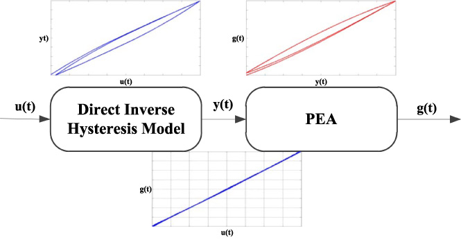
Feedforward controller in compensation of PEA.

2.1. CPI model

The equation of CPI model is defined as follows: $\begin{eqnarray}\displaystyle y(t)=au(t)+\displaystyle \mathop{\sum }_{i=1}^{n}p(i)H_{r(i)}[u](t). & & \displaystyle\end{eqnarray}$ (1)

Where, u(t) and y(t) are input and output functions respectively, u(t) ∈ C[0, T], y(t) ∈ C[0, T], a is a positive constant, H _{r (i)}[u](t) is output of play operator. Play operator is defined as follows: $\begin{eqnarray}\displaystyle H_{r(i)}[u](t)\text{} & =\text{} & \displaystyle z(t)=f_{\text{pop}}(u(t),r(i),z(t_{i}))\end{eqnarray}$ (2) $\begin{eqnarray}\displaystyle H_{r(i)}[u](0)\text{} & =\text{} & \displaystyle z(0)=f_{\text{pop}}(u(0),r(i),0).\end{eqnarray}$ (3)

For t _i < t ≤ t _i+1(i = 0, 1, 2, …, n −1) with $\begin{eqnarray}\displaystyle f_{\text{pop}}(u,r,z)=\max (u-r,\min (u+r,z)). & & \displaystyle\end{eqnarray}$ (4)

Where 0 = t ₁ < t ₂ < ⋯ < t _n = T are intervals in [0, T]. The relationship between input and output of play operator is shown in Fig. 2.

p(i) is weight constant, r(i) is threshold, i is from 1 to n, n is number of thresholds, r(i) is usually defined as follow [25–27]: $\begin{eqnarray}\displaystyle r(i)={\displaystyle \frac{i-1}{n}}\max |u(t)|. & & \displaystyle\end{eqnarray}$ (5)

Considering the fact that the PEA has the positive excitation nature, then one side operator is adopted. The one side operator is shown in Fig. 3 and defined as follows: $\begin{eqnarray}\displaystyle f_{\text{oop}}(u,r,z)\text{} & =\text{} & \displaystyle \max (u-r,\min (u,z))\end{eqnarray}$ (6) $\begin{eqnarray}\displaystyle H_{r(i)}[u](t)\text{} & =\text{} & \displaystyle z(t)=f_{\text{oop}}(u(t),r(i),z(t_{i}))\end{eqnarray}$ (7) $\begin{eqnarray}\displaystyle H_{r(i)}[u](0)\text{} & =\text{} & \displaystyle z(0)=f_{\text{oop}}(u(0),r(i),0).\end{eqnarray}$ (8)

Generally, u(t) is defined as input voltage and y(t) as output displacement in CPI model ((1)), therefore, using the model as feedforward controller needs to calculate the inversion of model. As mentioned in Fig. 1, u(t) and y(t) are defined as reference output displacement and control input voltage, the model is direct inverse model and can be used as feedforward controller directly to compensate the hysteresis of PEA. CPI model ((1)) is defined as the direct inverse model in this paper.

Fig. 2.

Play operator.

Fig. 3.

One side operator.

2.2. MDIPI model

CPI model is based on adding the product of the classical operators and the weight constants. One side operator with artificial setting threshold (5) is defined as the classical operator. The illustration of the classical operators of different threshold is shown in Fig. 4. From the basis of CPI model, the accuracy of model is depends on the selection of threshold. The threshold of artificial setting can not well describe the hysteresis loop, compared with optimal threshold. The threshold calculated by optimization algorithm is the optimal solution, which is calculated by global optimization according to the acquisition data of hysteresis loop. One side operator with the threshold calculated by optimization algorithm is defined as the modified classical operator in this paper.

Fig. 4.

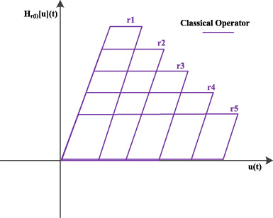
Illustration of classical operator.

One side operator with the rate threshold is defined as rate operator and used in rate dependent PI mode. The threshold value is proportional to the rate of input value, and the shape of the rate dependent operator is changed by rate threshold. The illustration of rate operator is shown in Fig. 5.

Fig. 5.

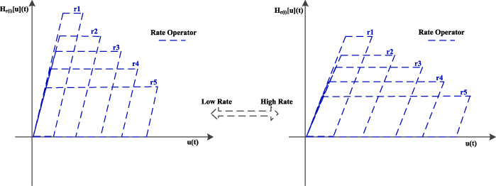
Illustration of rate operator.

According to Fig. 5, the shape of rate operator can be changed by threshold, the rate operator is rate dependent. Parameters of modified classical operator are calculated by optimization algorithm, all of them are constants, the modified classical operator is rate independent operator. The combination of rate dependent and rate independent operators is rate independent. Because the threshold of rate independent operator is constant, and the shape of rate independent operator is not changed by its threshold. The shape of the combination can not be completely changed only by changing the shape of rate dependent operator. So the combination is rate independent.

Single rate operator can not well describe the rate independent (i.e. static) hysteresis loop, because the threshold changes and leads to totally change of hysteresis loop. The combination of rate and modified classical operators is shown in Fig. 6. The combination can slightly change the shape of operators, which is useful in compensating the different amplitude trajectories.

Fig. 6.

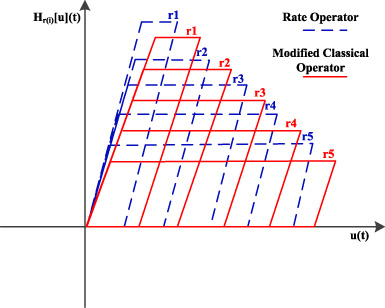
Combination of modified classical operators and rate operators.

Based on the basis of the combination of modified classical operators and rate operators, which is mentioned above, a modified direct inverse rate-independent Prandtl–Ishlinskii (PI) (MDIPI) model is proposed. The model has a linear part and two sets of operators including the rate operators and the modified classical operators. The MDIPI model is designed as direct inverse model and formulated in the following: $\begin{eqnarray}\displaystyle y(t)=a_{1}u(t)+a_{2}+a_{3}\displaystyle \mathop{\sum }_{i=1}^{n}p(i)H_{b_{ri}(t)}[u_{k}](t)+a_{4}\mathop{\sum }_{j=1}^{m}q(j)H_{d_{rj}}[u_{l}](t). & & \displaystyle\end{eqnarray}$ (9)

Where u(t) and y(t) are defined as reference output displacement and control input voltage. a ₁ and a ₂ are the constants of linear part, a ₃ and a ₄ are the constants of rate operators and modified classical operators respectively, p(i) and q(j) are the weight constants of rate operators and modified classical operators respectively. The rate threshold b _ri(t) and threshold calculated by optimization algorithm d _rj are defined as follows: $\begin{eqnarray}\displaystyle b_{ri}(t)\text{} & =\text{} & \displaystyle ib_{1}+abs\left(\frac{(u(t)-u(t_{i}))}{t-t_{i}}\right)b_{2}\end{eqnarray}$ (10) $\begin{eqnarray}\displaystyle d_{rj}\text{} & =\text{} & \displaystyle jd_{1}+d_{2}.\end{eqnarray}$ (11)

The two sets of operators of MDIPI model are defined same as expression of one side operator (6). The input of MDIPI model operators are expressed as $\begin{eqnarray}\displaystyle u_{k}(t)\text{} & =\text{} & \displaystyle u(t)k_{1}+k_{2}\end{eqnarray}$ (12) $\begin{eqnarray}\displaystyle u_{l}(t)\text{} & =\text{} & \displaystyle u(t)l_{1}+l_{2}.\end{eqnarray}$ (13)

Where b ₁, b ₂, d ₁, d ₂, k ₁, k ₂, l ₁, l ₂ are the constants. u _k(t) is input of rate operator and u _l(t) is input of modified classical operator.

The structure of MDIPI model is shown in Fig. 7. Compared with CPI model, MDIPI model has the properties of the adaption and accuracy, which are attributed to the combination of the rate operators and modified classical operators. The accuracy of compensation will be enhanced by the properties of MDIPI model in practical application.

Fig. 7.

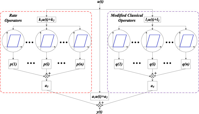
Structure of MDIPI model.

In previous works, the number of thresholds is usually defined as 10, the model with 10 operators has achieved better performance than the model with more or less than 10 operators [25–29,34], MDIPI model with two sets of operators, n = m = 10 in Eq. (9). How to determine the parameters and the performance of MIDPI model in compensating PEA will be introduced in next section.

3. Experimental validation of MDIPI model

3.1. Experimental setup

The diagram of experimental platform is shown in Fig. 8. The platform consists of PC with PCI board, piezoelectric controller (E621.SR, Physik Instrumente) with voltage amplifier and strain gauge sensor, piezoelectric actuator with strain gauge sensor (P-611.3S, Physik Instrumente), ADC (PCI-9203, OLP, china, 16bit, range: ±10 V) and DAC (PCI-9302, OLP, china, 16bit, range: ±10 V).

Fig. 8.

Block diagram of platform.

The gain of piezoelectric controller (PEC)is 10, PEC can amplify input voltage of DAC from 0–10 V to 0–100 V and drives the PEA, the maximum displacement of PEA is 100 μm at input voltage 100 V. The PEA displacement 0–100 μm is transferred by PEC position sensor as voltage and sampled by ADC from 0 to 10 V.

3.2. Identification of model parameters

To identify the parameters of MDIPI model, we choose sinusoidal signal as excitation, the signal is given by $\begin{eqnarray}\displaystyle y(t)=4\sin (2{\pi}ft+1.5{\pi})+4. & & \displaystyle\end{eqnarray}$ (14)

Where f is frequency and defined as 1, t ∈ [0,1], the sampling time is 0.001 s. y(t) is generated by DAC as input voltage, output displacement is acquired by ADC, the maximum output displacement is 80 μm according to Eq. ((14)). The identification equation is defined as $\begin{eqnarray}\displaystyle \bar{y(t)}=a_{1}u(t)+a_{2}+a_{3}\displaystyle \mathop{\sum }_{i=1}^{n}p(i)H_{b_{ri}(t)}[u_{k}](t)+a_{4}\mathop{\sum }_{j=1}^{m}q(j)H_{d_{rj}}[u_{l}](t). & & \displaystyle\end{eqnarray}$ (15)

$\bar{y(t)}$ is control voltage estimated by MDIPI model, u(t) is the output displacement, and the rest of Eq. ((15)) are defined same as MDIPI model ((9)). The object function is defined as $\begin{eqnarray}\displaystyle F(x)={\displaystyle \frac{1}{N}}\mathop{\sum }_{t=1}^{N}(y(t)-\bar{y(t)})^{2}. & & \displaystyle\end{eqnarray}$ (16)

Where N is number of experimental data, x is a set of identified parameters of MDIPI model. Genetic algorithm of matlab optimization tool box is used to find the effective parameters x that can minimize the object function F in Eq. (16). All the parameters of MDIPI model are calculated offline. Table 1 lists the 32 parameters of MDIPI model. The maximum absolute error and average absolute error are defined as Eq. (17) and Eq. (18) respectively, and abbreviated as MAE and AAE. $\begin{eqnarray}\displaystyle \text{MAE}\text{} & =\text{} & \displaystyle \max _{1\leq t\leq N}|u(t)-g(t)|\end{eqnarray}$ (17) $\begin{eqnarray}\displaystyle \text{AAE}\text{} & =\text{} & \displaystyle {\displaystyle \frac{1}{N}}\displaystyle \mathop{\sum }_{t=1}^{N}|u(t)-g(t)|.\end{eqnarray}$ (18)

Where u(t) is desired displacement, g(t) is actual displacement generated by PEA and N is the number of data.

Table 1

Identified parameters of MDIPI model

Number	p(i)	q(j)	a _i	b _i	d _i	k _i	l _i
1	1.05764	1.08578	1.41828	1.65441	1.33611	1.97713	0.96699
2	1.66537	1.14608	0.00698	0.00310	1.21779	0.75380	1.07411
3	2.20989	1.43726	−0.03299	-	-	-	-
4	0.77742	1.93752	1.23237	-	-	-	-
5	0.65245	1.52536	-	-	–	-	-
6	0.53791	1.14177	-	-	-	-	-
7	0.51385	1.68053	-	-	-	-	-
8	0.86577	1.14389	-	-	-	-	-
9	0.67672	0.93796	-	-	-	-	-
10	0.63595	0.94693	-	-	-	-	-

3.3. Results of experiment

The identification results of MDIPI model are shown in Fig. 9. Figure 9(a) is the hysteresis loops of experimental data and MDIPI model. Figure 9(b) shows the identification errors.

It is worthy to mention that the parameters of MDIPI model are identified by simple sinusoidal excitation signal (14), and MDIPI model is based on the operators (6). Using these parameters the MDIPI model can compensate the different amplitudes of reference signal.

Fig. 9.

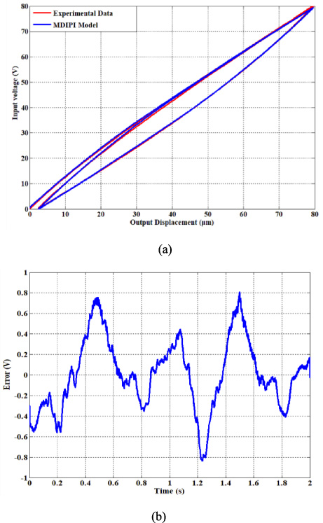
Identification of MDIPI model: (a) hysteresis loops; (b) identification errors.

To verify the performance of MDIPI model in compensation of desired reference displacement, we choose the complex displacement of PEA generated by known input voltage. The results are shown in Fig. 10. Figure 10(a) shows the complex displacement. Figure 10(b) shows the known input voltage and the control voltages of MDIPI model and CPI model. As shown in Fig. 10(c), MDIPI model well describes the relationship between displacement and voltage in both major and minor loops. Figure 10(d) gives the compensation errors of MDIPI and CPI models respectively. The MAE of MDIPI model is 1 μm and AAE is 0.38 μm, the MAE and AAE of CPI model are 2.47 μm and 0.72 μm respectively. Comparing with the errors of CPI model, all of the MDIPI model errors are reduced.

From the experimental results of the model performance verification, we can conclude that MDIPI model can be used as feedforward controller to compensate effectively the PEA hysteresis. From the compensation results, the MDIPI is more accurate than CPI model, and we can deduce that the accuracy of MDIPI model will be higher than that of CPI model in practical application of compensating reference trajectories.

Fig. 10.

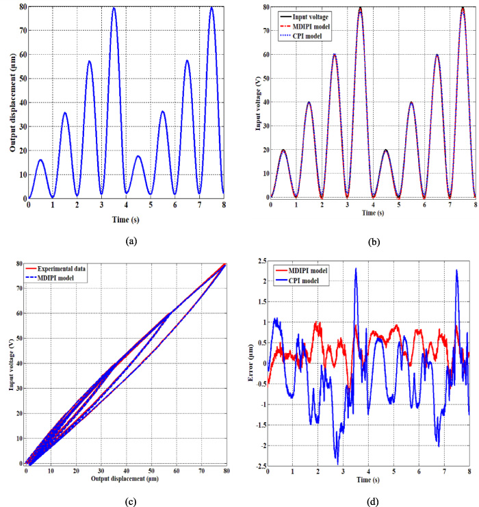
Compensation verification of MDIPI model in complex displacement: (a) displacement; (b) input voltages; (c) hysteresis loops; (d) compensation errors.

To verify the compensation performance of MDIPI model, we adopt different models including CPI, KP and Preisach models as comparison. CPI model is proposed in Eq. (1), KP and Preisach models are proposed in [8]. The compensation results of MDIPI model and the other models in complex trajectory are shown in Fig. 11. Figure 11(a) gives the actual displacements of different models and the reference displacement. The errors between output displacements of different models and reference displacement are shown in Fig. 11(b). Control voltages of different models are shown in Fig. 11(c). The relationship curves of different models between reference input and actual output displacements are shown in Fig. 11(d). From Fig. 11(d), we can see that MDIPI model is more linear than the other models. Table 2 gives the MAE and AAE of MDIPI model and the other models. The MAE and AAE of MDIPI model are 0.73 μm and 0.26 μm respectively. Comparing with KP, Preisach and CPI model, AAE of MDIPI model is reduced by 82%, 69% and 75% respectively. The MAE of MDIPI model is reduced by 3.63 μm, 1.91 μm and 2.98 μm respectively, compared with KP, Preisach and CPI model. The comparative experiments of complex trajectory compensation indicate that MDIPI model can improve the accuracy of compensating complex trajectory.

Fig. 11.

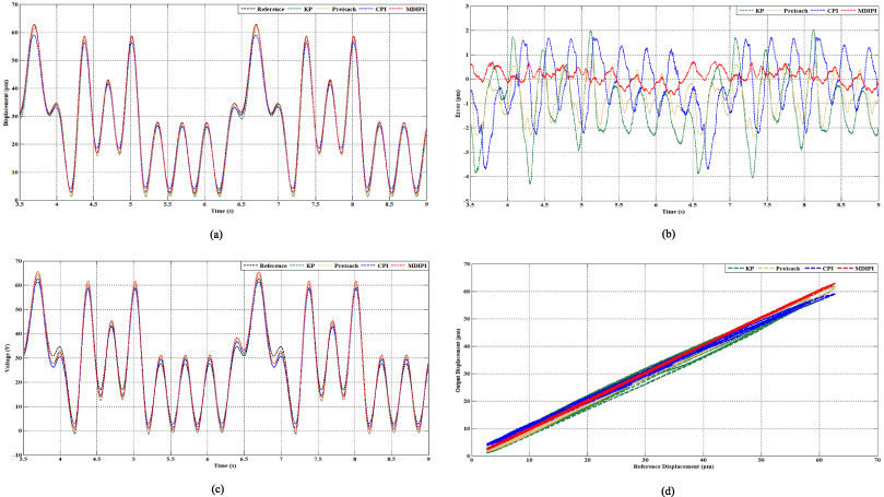
Performance of MDIPI model compensation in complex displacement trajectory: (a) displacements; (b) compensation errors; (c) control voltages; (d) compensation relationship curves.

Table 2

Compensation errors of complex trajectory

	KP model	Preisach model	CPI model	MDIPI model
AAE (μm)	1.41	0.85	1.06	0.26
MAE (μm)	4.36	2.64	3.71	0.73

The results of different models compensation in 60 μm p–p sinusoidal trajectory are shown in Fig. 12. The actual displacements of MDIPI, KP, Preisach and CPI models are shown in Fig. 12(a). Figure 12(b) shows the compensation errors of MDIPI and the other models. The control voltages of MDIPI and the other models are shown in Fig. 12(c). From Fig. 12(d), the relationship of MDIPI model is more near linearity than the other models. The MAE and AAE of different models are listed in Table 3. Comparing with KP, Preisach and CPI models, the AAE of MDIPI model is reduced by 82%, 78% and 89% respectively, the MAE of MDIPI model is reduced by 76%, 72% and 83% respectively. Form Tables 2 and 3, both AAE and MAE of MDIPI model are smaller than that of the other models, comparative experiments validate that the MDIPI model shows more superior performance in improving accuracy of compensating the complex and sinusoidal trajectories.

Fig. 12.

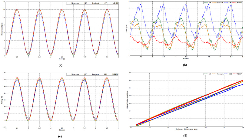
Performance of MDIPI model compensation in simple sinusoidal trajectory: (a) displacements; (b) compensation errors; (c) control voltages; (d) compensation relationship curves.

Table 3

Compensation errors of sinusoidal trajectory

	KP model	Preisach model	CPI model	MDIPI model
AAE (μm)	1.76	1.44	2.92	0.32
MAE (μm)	3.94	3.30	5.59	0.93

4. Conclusions

In this paper, a modified direct inverse rate-independent PI (MDIPI) model is proposed. Compared with the one set operators of CPI model, MDIPI model has two sets of operators including rate operators and modified classical operators. The MDIPI model has the properties of the adaption and accuracy, which are attributed to the combination of rate operators and modified classical operators. Because the thresholds of modified classical operators are calculated by optimization algorithm, and the modified classical operators are more accurate than the operators of CPI. Due to MDIPI model with the rate operators, it has the adaptive performance in compensating different peak trajectories. The MDIPI model can be used as feedforward controller to compensate different reference trajectories. Parameters of MDIPI model are calculated by matlab optimization tool box. The experiments of compensating the complex displacement trajectory and sinusoidal trajectory are validated on a commercial PEA platform. The experimental compensation results of complex trajectory show that AAE of MDIPI model is 0.26 μm. Comparing with KP, Preisach and CPI models, the AAE of MDIPI model in compensating complex trajectory is reduced by 82%, 69% and 75% respectively. The AAE of MDIPI model in the experiments of compensating sinusoidal trajectory is smaller than the other models as well. According to the compensation results in desired sinusoidal trajectory and complex trajectory, both AAE and MAE of MDIPI model are smaller than that of the other models. MDIPI model makes the relationship between reference displacement and output displacement near linearity, and it is effective in improving the accuracy of compensating reference trajectories of PEA.

Footnotes

Acknowledgements

This work was supported by the National Key R&D Program of China (No. 2017YFE0112100), EU H2020 Program (MNR4SCELL No. 734174), and “111” Project of China (D17017). This work was also partly supported by Changli Nano Biotechnology (China).

References

Leang

K.K.

and Devasia

, Feedback-linearized inverse feedforward for creep, hysteresis, and vibration compensation in AFM piezoactuators, IEEE Transactions on Control Systems Technology 15(5) (2007), 927–935.

Tao

and Zhu

, Hysteresis modeling with frequency-separation-based Gaussian process and its application to sinusoidal scanning for fast imaging of atomic force microscope, Sensors and Actuators A: Physical 311 (2020), 112070.

Clayton

G.M.

Tien

Leang

K.K.

, A review of feedforward control approaches in nanopositioning for high-speed SPM, Journal of Dynamic Systems Measurement and Control 131(6) (2009), 061101.

Salapaka

S.M.

and Salapaka

M.V.

, Scanning probe microscopy, IEEE Control Systems Magazine 28(2) (2008), 65–83.

Tian

, Hysteresis compensation of piezoelectric deformable mirror based on Prandtl–Ishlinskii model, Optics Communications 416 (2018), 94–99.

Lau

Liang

and Tan

, Enhanced robust impedance control of a constrained piezoelectric actuator-based surgical device, Sensors and Actuators A: Physical 290 (2019), 97–106.

Qin

Soundararajan

Jia

, Direct inverse linearization of piezoelectric actuator’s initial loading curve and its applications in full-fifield optical coherence tomography (FF-OCT), Mechanical Systems and Signal Processing 148 (2020), 107147.

Zhu

, Modeling and control of piezo-actuated nanopositioning stages: A survey, IEEE Transactions on Automation Science and Engineering 13(1) (2016), 313–332.

and Zhu

, An experimental comparison of proportional-integral, sliding mode, and robust adaptive control for piezo-actuated nanopositioning stages, Review of Scientific Instruments 85 (2014), 055112.

10.

Dong

Tan

and Xie

, Identification of micropositioning stage with piezoelectric actuators, Mechanical Systems and Signal Processing 75 (2016), 618–630.

11.

Zhang

, Implementable adaptive inverse control of hysteretic systems via output feedback, with application to piezoelectric positioning stages, IEEE Transactions on Industrial Electronics 63(9) (2016), 5733–5743.

12.

Chen

and Ozaki

, Adaptive control for plants in the presence of actuator and sensor uncertain hysteresis, IEEE Transactions on Automatic Control 56(1) (2011), 171–177.

13.

and Wang

, Parameter estimation of the Bouc–Wen hysteresis model using particle swarm optimization, Smart Materials and Structures 16(6) (2007), 2341–2349.

14.

Zhang

Guo

, Sliding mode tracking control with perturbation estimation for hysteresis nonlinearity of piezo-actuated stages, IEEE Access 6 (2018), 30617–30629.

15.

Zhou

Yang

Wang

, Adaptive sliding mode control based on Duhem model for piezoelectric actuators, IETE Technical Review 33(5) (2016), 557–568.

16.

Zhang

and Ma

, Development of a combined Prandtl Ishlinskii–Preisach model, Sensors and Actuators A: Physical 304 (2020), 111797.

17.

Janaideh

M.A.

Rakotondrabe

and Aljanaideh

, Further results on hysteresis compensation of smart micropositioning systems with the inverse Prandtl–Ishlinskii compensator, IEEE Transactions on Control Systems Technology 24(2) (2016), 428–439.

18.

Al-Nadawi

Y.K.

Tan

and Khalil

H.K.

, Inversion-free hysteresis compensation via adaptive conditional servomechanism with application to nanopositioning control, IEEE Transactions on Control Systems Technology 29(5) (2021), 1922–1935.

19.

Janaideh

M.A.

and Krejčí

, An inversion formula for a Prandtl–Ishlinskii operator with time dependent thresholds, Physica B 406(8) (2011), 1528–1532.

20.

Janaideh

M.A.

and Aljanaideh

, Further results on open-loop compensation of rate-dependent hysteresis in a magnetostrictive actuator with the Prandtl–Ishlinskii model, Mechanical Systems and Signal Processing 104 (2018), 835–850.

21.

Janaideh

M.A.

Rakheja

and Su

, A generalized Prandtl–Ishlinskii model for characterizing the hysteresis and saturation nonlinearities of smart actuators, Smart Materials and Structures 18(4) (2009), 045001.

22.

Sayyaadi

and Zakerzadeh

M.R.

, Position control of shape memory alloy actuator based on the generalized Prandtl–Ishlinskii inverse model, Mechatronics 22(7) (2012), 945–957.

23.

Xie

Ren

and Wang

, A modifified asymmetric generalized Prandtl–Ishlinskii model for characterizing the irregular asymmetric hysteresis of self-made pneumatic muscle actuators, Mechanism and Machine Theory 149 (2020), 103836.

24.

Xie

Mei

Liu

, Hysteresis modeling and trajectory tracking control of the pneumatic muscle actuator using modified Prandtl–Ishlinskii model, Mechanism and Machine Theory 120 (2018), 213–224.

25.

Yang

and Zhu

, Real-time inverse hysteresis compensation of piezoelectric actuators with a modified Prandtl–Ishlinskii model, Review of Scientific Instruments 83(6) (2012), 065106.

26.

Gan

Zhang

and Wu

, A Generalized Prandtl–Ishlinskii model for characterizing the rate-independent and rate-dependent hysteresis of piezoelectric actuators, Review of Scientific Instruments 87(3) (2016), 035002.

27.

Qin

Tian

Zhang

, A novel direct inverse modeling approach for hysteresis compensation of piezoelectric actuator in feedforward applications, IEEE/ASME Transaction on Mechatronics 18(3) (2013), 981–989.

28.

Hwang

Chae

, Direct identification of generalized Prandtl–Ishlinskii model inversion for asymmetric hysteresis compensation, ISA Transactions 70 (2017), 209–218.

29.

Qiu

Jiang

and Ji

, A modified Prandtl–Ishlinskii model and its applications to inverse control of piezoelectric actuators, Computers Materials & Continua 26(1) (2011), 1–18.

30.

Zhang

Merced

Sepúlveda

, Optimal compression of generalized Prandtl–Ishlinskii hysteresis models, Automatica 57 (2015), 170–179.

31.

Qin

Zhao

and Zhou

, Modeling and identification of the rate-dependent hysteresis of piezoelectric actuator using a modified Prandtl–Ishlinskii model, Micromachines 8(4) (2017), 114.

32.

Tao

and Zhu

, Rate-dependent hysteresis modeling and compensation of piezoelectric actuators using Gaussian process, Sensors and Actuators A: Physical 295 (2019), 357–365.

33.

Yang

, A two-stage model for rate-dependent inverse hysteresis in reluctance actuators, Mechanical Systems and Signal Processing 135 (2020), 106427.

34.

Jiang

Qiu

, A modified Prandtl–Ishlinskii model for modeling asymmetric hysteresis of piezoelectric actuators, IEEE Transactions on Ultrasonics, Ferroelectrics, and Frequency Control 57(5) (2010), 1200–1210.

35.

Zhu

and Su

, Modeling and compensation of asymmetric hysteresis nonlinearity for piezoceramic actuators with a modified Prandtl–Ishlinskii model, IEEE Transactions on Industrial Electronics 61(3) (2014), 1583–1595.

36.

Wang

Chen

, A new hysteresis modeling and optimization for piezoelectric actuators based on asymmetric Prandtl–Ishlinskii model, Sensors and Actuators A: Physical 316 (2020), 112431.