
Abstract
In this paper CNNs are used for solving an optimization problem with two different approaches: CNN is used as a surrogate model of the forward problem, inserted in an optimization loop governed by a genetic algorithm, in the first approach, while a CNN is trained for solving directly the inverse problem in the second approach. The case study is the shape design of a magnetic core used for material testing.
Introduction
In the area of non-destructive testing, a magnetic field is applied to the object under test and any resulting changes of magnetic flux in the region of interest can be detected. Either direct or alternating fields can be applied. Localized phenomena such as surface or sub-surface cracks in ferrite steels can be detected by means of a flux linkage variation [1–7]. In this contest, the shape design of the magnetic core of the electromagnet is particularly important in view of a deep and homogenous flux density induced in the material under test. Traditionally, the problem is treated in terms of optimization procedures based on Finite Element Method (FEM) for the field analysis. Recently, deep learning techniques have been used to build surrogate models for field analysis of electromagnetic devices [8–10]. Convolutional Neural Networks (CNNs) are neural networks which allow to evaluate a field quantity (either a value or a vector of values like e.g. a field distribution), starting from an image [10,11]. The training of these CNNs is usually done with numerical analyses and in particular the FEM is used. Once a neural network is trained, it can be used as a surrogate model and inserted in an optimization loop. This way, the computational burden is limited to the net training, while the evaluation of the field quantities during the optimization loop is rather inexpensive. Another fascinating and innovative way to use CNNs for solving optimization problems is to invert the net: given a field quantity or distribution, geometry is drawn by the net [12]. To this end, transposed 2D convolution layers are used in the net solving the inverse problem. In this paper, these new approaches are applied to an optimization problem of shape design of an iron core used for material testing.
The case study
Let us consider an iron-cored electromagnet which is widely used in magnetic non-destructive testing of ferromagnetic materials. It is assumed that the electromagnet is operated by DC and with adjustable geometry. The electromagnetic device is schematically shown in Fig. 1 (due to the symmetry, only right part is shown). The sensitivity of detection for any portion of a component being tested varies not only with the distance between the pole pieces but also with the shape of the ferrite core. Hence, correct design of the overall unit is essential in order to ensure the highest system sensitivity. The question we ask is as follows: what is the electromagnet’s optimal shape when applying it for energizing a magnetic field in a ferrite steel plate under test. It is obvious that the magnetic flux density should be as high as possible on the reverse side of the plate under test.
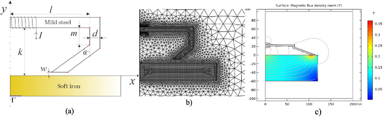
(a) Geometry of the iron core electromagnet with ferrite steel plate, the sampling points (blue dots) for the magnetic induction field are highlighted (b) exemplary finite element mesh (c) magnetic field map.
In order to reduce the computational burden, after neglecting the edge effects, the field analysis can be done by using a simplified 2D FEM model. Such an approach is commonly used in practice, when at the beginning a rough solution is achieved by using a 2D model, and then final 3D model could be built around the previously obtained results [13,14]. Comsol Multiphysics software is used and a magnetostatic problem is solved [15]. In Fig. 1(b), an exemplary finite element mesh is shown. The mesh used for calculations consists of around 55,000 elements. The calculation domain has been truncated by applying the infinite elements on the outer edge of the calculation area. In the calculations it is assumed that the electrical parameters of the coil are: electrical conductivity 60 MS/m, number of coil turns N = 500, wire diameter w d = 0.5 mm. For the purpose of reducing the computational cost, the subsequent calculations have been performed with linear materials, i.e. μ r = 2000 was taken for the iron-cored electromagnet, while μ r = 1000 for the ferrite steel plate.
In a single optimization process the iron core electromagnet geometry is adjustable with the help of four design variables, i.e.: k, l, m and 𝛼, whereas core thickness d, and air gap w, are constant.
Since the core geometry greatly affects the detection sensitivity of the device, the problem is to find the optimal core shape which gives the maximum average value of magnetic flux density on the reverse side of the slab under test (boundary Γ).
The region of interest, the boundary Γ, is defined as in Fig. 1a. The magnetic flux density is evaluated in ten points on the boundary Γ. Four design variables x = [k, l, m, 𝛼] are considered (see Fig. 1). The variation range of the design variables is shown in Table 1.
Variation range for the design variables
Variation range for the design variables
The objective function f is defined as follows
For the sake of a comparison, the optimization problem has been first solved in a classical way: a genetic algorithm is applied and the field analysis is performed with FEM.
As an optimization tool a modified version of the GA presented in [16] has been implemented in MATLAB, while the field equations have been solved in Comsol Multiphysics software. At the beginning of the optimization process, genetic algorithm parameters, electromagnetic core parameters, the objective function (as a magnetic field density B), and limitations are defined. Next, with the help of floating point number generator, the initial population is randomly generated and encoded. Objective function is calculated for all the candidates. Next, a selection process is then carried out, which in this case bases on roulette-wheel selection. In all the cases selection coefficient is equal to 0.5, which means, that exactly half of the population size passes to the next process called crossover. After the crossover process, random changes are introduced (i.e. mutation). The purpose of the introduced random variations is to improve candidates, making them into more efficient solutions. The mutation rate in all the cases has been set to 0.2. Digital offsprings go to the next generation and become a new set of candidate solutions, which are subjected to the second round of objective function evaluation. This process repeats. The expectation is that the average objective function value of the population will increase each round, and so by repeating this process very good solutions to the problem will be obtained. The process stops when the maximum number of generations is reached and finally the best solution is stored. The flowchart of the optimization procedure is shown in Fig. 2.
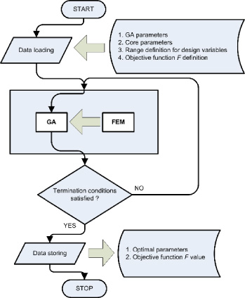
The flowchart of the optimization procedure.
In order to solve the optimization problem, two different approaches are implemented: the forward and the inverse approach. In the forward approach, the field analysis is based on a surrogate model and a genetic algorithm is applied for solving the optimization problem [17]. The objective function used by the optimization algorithm is evaluated by means of the surrogate model. In the inverse approach a surrogate model of the inverse problem is performed.
To this end, two CNNs are built and trained. The first CNN (CNN-1), relevant to the forward approach, receives an image of the geometry as input and returns the magnetic field profile along Γ boundary as output. The genetic algorithm uses the CNN-1 for the objective function evaluation.
In turn, the second CNN (CNN-2), relevant to the inverse approach, receives the vector of the magnetic field profile prescribed along Γ boundary and returns the corresponding geometry image of the iron core.
For implementing the CNN approach, an appropriate database has been built by solving, with the help of FEM, 25,000 geometries for the forward approach (CNN-1) and 70,000 for the inverse approach (CNN-2). As far as the definition of a suitable control region, a sub-domain Ω c is considered (see Fig. 3a): for each analyzed geometry the corresponding image of 80 × 140 pixels representing Ω c is stored with the relevant magnetic field profile. The resolution is chosen in a way on one hand to reduce the number of pixels as much as possible and, on the other hand, to be able to appreciate the image details.
The stored image relevant to Ω c contains only the core of the device, cutting out the slab and the feeding coil, and it is a black/white image (matrix composed of 1 or 0 entries). In Fig. 3 both the images of the domain of the FEM and the corresponding image, with lower resolution and stored in the database, are shown.
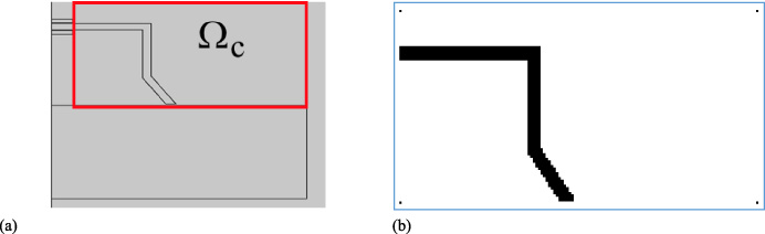
Example of a possible geometry: image of the domain of the FEM, the control sub-region is highlighted (a) and B/W image 80 × 140 pixels (b).
The convolutional neural network CNN-1 is composed of 18 layers, in which 4 blocks can be highlighted. Each block is composed of a convolutional layer, a batch normalization layer [18] and a Rectified Linear Unit ReLU function, as shown in Table 2.
The ReLU function is one of the most used activation function for CNN because it showed good performances in training this kind of neural networks in terms of avoiding overfitting [11].
CNN-1 structure
CNN-1 structure
The convolutional layers are characterized by filters of size 3 × 3. The number of filters vary from 8 to 32, depending on the block. Two average pooling layers with filter of size 2 × 2 are applied in order to obtain a more stable solution.
At the end of the structure a dropout layer is used and a fully connected layer followed by the regression layer allows to obtain a vector of 10 elements as output.
Since there are relatively few input data (field vector 1 × 10) while the output data are more than 11,000 values (image matrix), a typical upsampling problem should be handled, in view of a reliable training.
To this end, the convolutional neural network CNN-2 is composed of 25 layers, three of which are transposed 2D convolutional layers, while the same block as in CNN-1 is used 7 times. Transposed convolutional layers are used to upsample the input vector. The transposed convolution operation implements the convolution operator on a modified (enlarged) input image. Hence, given an input image and a filter, the input image is first modified by inserting zeros in between rows and columns and eventually around the input image. Then, the filter is applied to this enlarged image i.e. the filter is slided across the image, implementing the convolution operator. The result of this operation is an image as output which is larger than the input image.
The CNN-2 structure is represented in Table 3.
CNN-2 structure
CNN-2 structure
A quantitative method for evaluating the goodness of the net training is the mean square error e calculated on the validation set as
A qualitative method to grasp the goodness of the trained net is to plot the true values versus the predicted values e.g. for the training set. The more the points are close to the diagonal line, the more the model prediction is accurate.
The net CNN-1 has been trained with n = 25,000 samples, n t = 23,000 of which for the training set and n v = 2000 for the validation set. The training lasted 200 epochs and the Stochastic Gradient Descent with Momentum (SGDM) method has been applied for training.
The mean square error obtained after training the net is 0.04.
The results relevant to CNN-1 are shown in Fig. 4.
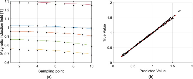
(a) Magnetic induction field FEM solutions (coloured continuous line) and predicted values (black star) for different geometries, (b) true values vs predicted values for the validation set.
Figure 4 shows how the net is able to predict the field profile, given the image of the geometry. In Fig. 4a a comparison between true values of field profile i.e. FEM results and values predicted by the network after training is performed for different geometries. In turn in Fig. 4b the distribution of true values versus predicted values is plotted for all points in the validation set: apparently all points are very close to the diagonal (red dashed line) thus showing a good agreement between true and predicted values.
For the sake of a comparison, the optimization problem has been first solved in a classical way: the genetic algorithm described previously is applied and the field analysis is performed with FEM, no network was resorted to. The optimization was based on 12 individuals and run for 150 iterations. The exemplary effects of optimization have been shown in Fig. 5a, whereas results in numerical form have been summarized in Table 4.
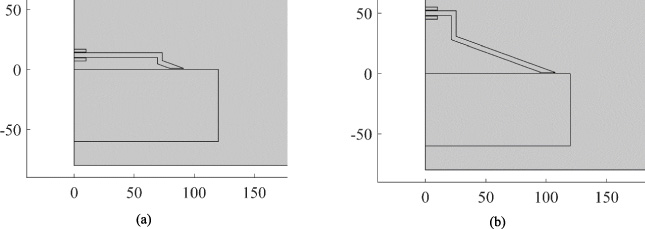
Results of the genetic algorithm: optimal geometry obtained with the objective function calculation based on (a) FEM, (b) CNN-1.
Subsequently, the same genetic algorithm with the same settings (i.e. 12 individuals and 150 generations) is run but the objective function is now calculated by means of CNN-1, previously trained with FEM. However, during this optimization, no FE calculations are performed.
The optimized geometry so found is shown in Fig. 5b and described in Table 4.
The relevant optimal design variables and objective function are shown in Table 4.
Optimization results of the forward approach
The * indicates that the optimal value of the objective function is re-calculated by FEM, even though the optimization is based on the CNN-1.
As can be noted form Table 4, the values of the objective function obtained with the two methods are close, but the relevant device geometries are different.
The net has been trained with n = 70,000 samples, n t = 60,000 of which for the training set and n v = 10,000 for the validation set. The training lasted 100 epochs and the ADAptive Moment estimation (ADAM) method has been applied for training.
The mean square error obtained after training the net is 0.042.
CNN-2, after being trained, is able, given a field profile of 10 values as input, to find a cloud of grey and black pixels as shown in Fig. 6b.

Example of (a) input and (b) output of CNN-2.
In Fig. 6b the drawing of “true” geometry which gives rise to the field profile in Fig. 6a is over posed to the cloud found by the net.
As can be noted in Fig. 7, given two different profiles, the net is able to find two different geometries.
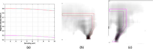
Examples of (a) input and (b) output of CNN-2 regarding two different field profiles.
When the CNN is fed by similar field profiles, similar output (similar clouds) is found. However, different geometries gave rise to similar profiles, as shown in Fig. 8.
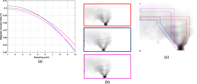
Example of (a) input (similar field profiles), (b) output (similar clouds) of the CNN-2 and (c) output cloud with the “true” geometries super imposed.
From the Figs 6–8 it can be noted that the there is a part of the output image, specifically a subset of pixels belonging to the shaded cloud, which is darker than the rest of the cloud. This means that there is a more likely probability that the geometry is in that part of the domain: it appears that the position d of the final part of the core (see Fig. 8c) is correctly identified in most of the cases. Also the angle 𝛼 appears to be well identified because the grey cloud is shaped rather precisely in the subregion close to the pole.
It can be stated that the grey cloud represents a kind of probability density function helping to identify the topology of the core, where the grey scale is an indicator of probability. Unfortunately, the CNN is not able to find a unique geometry, given a field profile. This issue is due to the ill-posedness of the problem: because different geometries can give rise to very similar profile, it is not always possible to find a unique geometry, given a field profile [19].
In recent papers and in this work, CNNs are showing good capabilities to work as surrogate models in electromagnetics, mimicking field analysis. However, further studies are needed to investigate the computational burden, relevant to the net training, compared to an optimization based on FEMs.
A further approach is proposed in the paper: to use a CNN for solving directly the optimization problem, without the use of FE analysis neither of an optimization algorithm. The CNN is able to reconstruct a cloud of probability density to find the geometry in the given pixel of the cloud. However, due to the ill-posedness of the problem, the CNN is not able to find the correct geometry.
All in one, the paper, by comparing the two different approaches based on CNNs, aims to go one step further in the direction of deep learning applied to optimization problems in electromagnetism.