Identification of moisture inside walls in buildings using machine learning and ensemble methods

Abstract

According to the article, locating moisture within the walls of buildings using electrical impedance tomography is discussed in detail. The algorithmic approach, whose role is to convert the input measurements into images, received excellent attention during the development process. Numerous models have been trained to generate tomographic images based on individual pixels in a given image based on machine learning methods. An array of categorisation data was then generated, which enabled the development of a classification model to solve the problem of optimal model selection for a given point on the screen. It was achieved in this manner by developing a pixel-oriented ensemble model (POE), the goal of which is to provide tomographic reconstructions of at least the same quality as homogeneous algorithmic approaches. Artificial neural networks (ANN), linear regression (LR), and the long short-term memory network (LSTM) were employed in the current research to get homogeneous machine learning results. An image reconstruction algorithm such as the ANN or the LR reconstructs the image pixel by pixel, which means that a different prediction model is trained for each image pixel. In the case of LSTM, a single network is responsible for creating the entire image. Then, using the POE algorithm, the best reconstruction method was fitted to each pixel of the output image while considering the measurement scenario provided to the program. As a result, each measurement consequences in a unique assignment of reconstructive procedures to individual pixels, which is different for each measurement. It is the capacity to maximise the selection of a prediction model while considering both a given pixel and a specific measurement vector that distinguishes the provided POE concept from other approaches.

Keywords

Electrical tomography moisture detection machine learning neural networks long short-term memory (LSTM)

1. Introduction

The research described in this paper is motivated by the need to improve the methods of imaging the walls’ interior to detect areas of increased humidity. The most common reasons for damp walls caused by water infiltration from the outside are inadequate insulation and foundations, roof leakage, an inadequate rainwater drainage system, and deficiencies in sheet metal work. The primary cause of moisture problems inside a building is inadequate thermal insulation of the walls, which allows moisture to accumulate and not be discharged to the outside. In the winter, moisture condenses on frozen walls due to the warmer indoor air. Additionally, inadequate ventilation of the rooms may result in residual moisture, which creates an unpleasant microclimate that is unhealthy for the occupants. Inadequate foundation insulation frequently results in moisture penetration into the walls. It occurs due to poorly drained ground or rainwater seeping through horizontal or vertical insulation leaks. Changes in groundwater levels may occur due to a capillary rise of moisture from the ground or as a result of direct or indirect rainwater action. Water that has permeated the wall during the winter months freezes, increasing the volume. It may result in the collapse of the building’s foundations and partitions. In general, groundwater is not chemically neutral. It contains dissolved substances, most frequently chlorides, sulphates, and nitrates, potentially toxic chemically. Capillary rise allows water with dissolved compounds to reach the higher parts of the walls, causing salt blooms, discolouration, peeling of paint coatings, and plaster peeling. Chemical corrosion may be caused by dissolved chemical substances from the ground or, for example, from preparations protecting the roof truss. Corrosion caused by biological organisms is just as dangerous.

Additionally, the damp walls (both inside and outside) provide an ideal environment for the growth of fungi and mould. All of this contributes to the walls’ unsightliness. Additionally, the materials that comprise the structure of the building, i.e., the so-called biodeterioration of concrete, glass, bricks, mortars, and wood, among others, Moisture in building walls affect the health of occupants, as the presence of mould and fungi in rooms can cause allergies and respiratory diseases.

The currently used methods of measuring the moisture inside the porous brick walls enable point measurements. However, there are no methods to visualise the moisture distribution inside the walls [1]. With the help of tomography, it can create 2D and 3D models from the measurements. Moisture remaining inside the walls of buildings has many negative effects, which concern both the material, construction, aesthetic, and ecological spheres and issues related to the health of people staying in damp rooms [2,3]. The adverse effects include a decrease in the thermal insulation of wet materials, a decrease in the strength of materials and the load-bearing capacity of masonry structural elements, biological corrosion, erosive processes associated with salt-action, an increase in repair costs, and an increased risk of respiratory diseases [3–5].

Electrical impedance tomography (EIT) is a type of tomography suitable for creating visualisations of moisture areas in walls [6]. This feature distinguishes tomography from known point methods, e.g., gravimetric, dielectric or microwave [7]. The gravimetric method as an invasive method is considered the most accurate, but it is a destructive method. For this reason, it cannot be used, for example, in historical buildings that are subject to legal protection. The element that distinguishes tomography from other methods is the goal it pursues. Therefore, the purpose of tomography is not to precisely (in per cent) determine the water content at individual points of the tested wall. Instead, tomography enables the imaging of wet areas against a dry background. Apart from the software, it needs a high-quality tomograph consisting of electrodes and electronic systems to perform tomographic reconstructions. There are many kinds of tomography, such as computed tomography (CT) [8], electrical capacitance tomography (ECT) [9–14], electrical resistivity tomography (ERT) [15–17], X-rays [18], ultrasound [19], magnetism [20–22], visible light [23], etc. This work deals with software that transforms measurement data into the colours of pixels (finite elements) that make up the reconstruction images. This problem is called ill-posed [24,25]. From the algorithmic point of view, tomography uses direct and iterative methods, often related to machine learning. The direct methods include Total Variation [26], Level Set [27], Gauss-Newton with Tikhonov or Laplace regularisation [3], and others. Machine learning methods include Logistic Regression [28], Elastic Net [3,26], Least Absolute Shrinkage and Selection Operator (Lasso) [3], Linear Regression and Least-Angle Regression (LARS) [3], Artificial Neural Networks (ANN) [3,26], sparse Bayesian learning (SBL) [25,29,30], etc.

The research aimed to develop an effective method for detecting moisture inside walls. We created an original, heterogeneous method of transforming electrical impedance tomography (EIT) measurements into images of moisture distribution [26]. The course of the research included the performance of validation measurements on an authentic brick wall. The way of performing validation measurements using direct and indirect point methods is presented in article [2] in Section 2.2.. Validation Measurements. Then the Pixel-Oriented Ensemble (POE) method was designed, and the machine learning model was trained. Three homogeneous regression models were trained: ANN, LR, and LSTM. Then the classification neural network model was trained. In the last stage, reconstruction images were generated based on simulation data, and the hybrid POE method was compared with homogeneous methods. Known quantitative indicators were used for comparison.

2. Materials and methods

2.1. Data preparation and validation

The traditional approach to developing mathematical models considers forward problems, which in the case of electrical tomography means determining the values of voltage measurements made on the wall surface using the known electrical conductivity of the tested object. Tomography’s purpose is quite the opposite. It determines the electrical conductivity of individual components within the monitored object using surface measurements. It is an ill-posed problem because it may be impossible to find a true solution due to insufficient or excessive data. Inverse problems are frequently ill-posed problems, and their resolution requires regularization methods or machine learning. The generalized Laplace equation can be used to represent the following EIT forward problem: ${\nabla}\cdot ({\sigma}{\nabla}u)=\sum _{i=1}^{3}\frac{\partial }{\partial x_{i}}({\sigma}\frac{\partial u}{\partial x_{i}})=0$ , $\frac{{\omega}{\varepsilon}}{{\sigma}}\ll 1$ , where σ—electrical conductivity, u—electric potential, ω—angular frequency, ϵ—permittivity.

Suppose that F defines a transformation function from inputs x to the set of outputs y, such that F (x) = y. The inverse problem is to use the (most often noisy) data obtained from a non-linear or linear F function to reconstruct (recover) some set of unknown parameters of the x model. Unfortunately, this kind of inverse mapping or function usually does not exist. Therefore, a series of numerical approximations must be made to find the closest solution. Furthermore, if the inverse problem does not depend continuously on the data, it will be very sensitive to changes in boundary measurements. This condition leads to wrongly posed inverse problems. Contrary to the well-posed EIT forward problem, the inverse EIT problem is severely ill-posed and extremely sensitive to small disruptions in the data boundary. For this reason, even a moderately noisy data set can make it difficult to find meaningful solutions [31].

Corresponding algorithms were developed to train machine learning-based models. The Eidors toolbox and the finite element method were used [32,33]. A training set of 14152 observations was generated. The input vector contained 96 measurements equivalent to the voltage drops between the specific electrode pairs. 16 specially designed electrodes are placed linearly on a metal strip. The spatial image is created on 4955 elements (pixels) finite element mesh. The same training data was used to train all the models considered in this research. The method of preparing the simulation data has been described in detail in publication [3] in Section 2.1.. Selected Hardware Issues, Sample Models, and Reconstructions.

Figure 1 shows one of the 14152 generated cases used to train the predictive system. A wall sector in Fig. 1a contains a random piece of moisture. Thanks to the variety of colors on the finite element mesh, the wet part is visible. On the vertical axis of Fig. 1b, we see the input vector values (measurements) expressed in arbitrary units, which are closely correlated with the voltages measured between the individual pairs of electrodes. The 4955 conductivity values are assigned to 96 voltage-like measurements called arbitrary units. The arbitrary units change in the range (−0.02 ÷ +0.06) as the polarity of the electrodes changes during individual measurements. The value of each measurement was increased by adding Gaussian noise with a standard deviation of 4%. The image’s finite elements (pixels) have 1 for the background (drywall) or 10 for the moist wall.

Fig. 1.

A sample training measurement case generated with the Eidors toolbox: (a) – a wall section with a wet upper part; (b) – 96 measurement values corresponding to the wet section.

The parameters of the simulation algorithm were validated based on actual measurements performed on a specially designed test stand (Fig. 2).

Fig. 2.

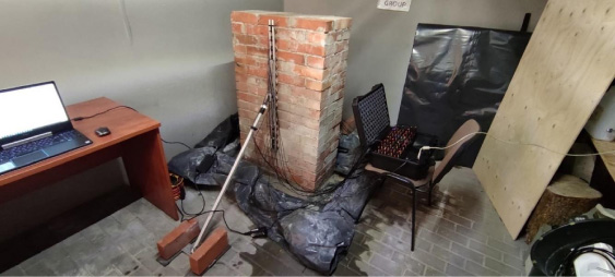
EIT measurement station. A metal strip with EIT electrodes was placed against the brick wall. On the right side, one can see the tomograph on the chair.

2.2. Artificial neural network (ANN)

An artificial neural network was used in the research, and strictly speaking, it was a multilayer perceptron. The network consisted of 96 input measurements, 10 neurons in the hidden layer, and one in the output layer. Since the spatial tomographic image consisted of 4955 finite elements (pixels), this number of single-output neural networks (96 −10 −1) × 4955 was trained. All neural networks were identical in structure. Randomised observations in the training set were applied before each training process. The Levenberg-Marquardt algorithm was used to train the network. Two network quality assessment criteria were used during the training process: mean square error (MSE) and regression (R-value). The hyperbolic tangent transfer function in the hidden and output layers was used. The early stopping method was used to prevent overfitting the neural network. This method consists of the fact that the training process is stopped if, after 6 successive iterations, the MSE error for the validation set does not decrease. Figure 3 shows the learning process through the mean squared error values for the validation, testing, and training sets.

Fig. 3.

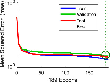
Training ANN for a randomly selected pixel. The best validation performance is 2.1965 at epoch 183.

The shape of all 3 curves resembles a hyperbola. The minor errors characterise the training blue line. The test and validation lines are slightly more error-prone, but the differences are insignificant. All this proves a minimal risk of overfitting the network and, thus, the trained model’s high quality and ability to generalise. The entire set of cases has been divided into 3 sets: training, validation, and testing, in the proportion of 70:15:15. It means that the training set consisted of 9906 cases, and the validation and test sets each had 2123 cases.

2.3. Linear regression model (LR)

Another homogeneous machine learning method was linear regression LR. The 96-dimensional vector of input data was optimised using the LR technique. The learner used it as a support vector machine. The model also uses regularisation for Lasso (Least Absolute Shrinkage and Selection Operator). The algorithm adds the absolute magnitude of the coefficient to the loss function as a penalty component. The Lasso cost function is defined by formula (1) $\begin{eqnarray}\displaystyle \min _{{\beta}_{0},{\beta}}\left(\frac{\mathop{\sum }_{i=1}^{n}(y_{i}-b-\boldsymbol{x}_{i}^{T}{\beta})^{2}}{2n}+{\lambda}\mathop{\sum }_{j=1}^{p}|{\beta}_{j}|\right). & & \displaystyle\end{eqnarray}$ (1) In (1) $x_{i}^{T}$ is a transposed vector of length p at observation i and y_i is the reconstruction of a pixel at observation i where n is the number of observations. The regularisation parameter lambda (𝜆 ≥ 0) is used and is considered case 𝜆 =1∕n. The parameter b is a scalar bias, a p-dimensional vector. The number of non-zero parameters decreases as Lambda grows. The L2 ridge regression cost function, which may be employed instead of Lasso, is shown in Formula (2) $\begin{eqnarray}\displaystyle \min _{{\beta}_{0},{\beta}}\left({\displaystyle \frac{\mathop{\sum }_{i=1}^{n}(y_{i}-b-\boldsymbol{x}_{i}^{T}{\beta})^{2}}{2n}}+{\displaystyle \frac{{\lambda}}{2}}\mathop{\sum }_{j=1}^{p}{\beta}_{j}^{2}\right), & & \displaystyle\end{eqnarray}$ (2) where x is an observation of p predictors, is a vector of p coefficients, and b is a bias, was the loss function for a linear regression model type. The loss function is calculated as MSE in the implemented method and can be expressed as ℓ[ y , f ( x )] = max[0, | y − f ( x )|−ϵ], where y ∈ (−∞, ∞) is a vector of response/reconstruction values. Regularised SVM regression is included in LR model. The model decreases computation time by minimising the objective function using the stochastic gradient descent (SGD) formula. SVM with a ridge penalty is used in this technique, which is optimised using dual SGD for SVM. The criteria to complete the iteration process is the formula ${\varkappa}>\Vert \frac{B_{t}-B_{t-1}}{B_{t}}\Vert$ . 𝜘 represents relative tolerance on linear coefficients ${\beta}_{t}^{\prime }$ , bias term b_t, and $B_{t}=[{\beta}_{t}^{\prime },b_{t}]$ . For all training procedures, deviance b is the y-weighted median. The learning rate 𝛾 is an important hyperparameter. If the regularisation in the algorithm is Lasso, then 𝛾 and i are constant for all iterations. 𝛾 specifies the starting learning rate 𝛾₀ if regularisation is L2 (ridge). According to iteration i the program calculates the learning rate (3) $\begin{eqnarray}\displaystyle {\gamma}_{i}={\displaystyle \frac{{\gamma}_{0}}{(1+{\lambda}{\gamma}_{0})^{c}}}. & & \displaystyle\end{eqnarray}$ (3) If the solver used is a stochastic gradient descent (SGD), then c = 1, but if the solver used would be the average SGD (ASGD), then c = 2∕3, but if the learner is an SVM (like in the considered case), then c = 3∕4. As with the ANN, the LR models were trained separately for each pixel of the reconstruction image. It can be written as (96 − LR −1) × 4955.

2.4. The long short-term memory network (LSTM)

For the LSTM network, the same proportion of the dataset division was used as in the case of ANN, i.e., 70:15:15 (training, validation, and testing sets). Since the “early stopping” method was not used for LSTM, and thus there was no need to use the validation set, this set was added to the training set. So, the training set used to train the LSTM network was enlarged to 12029 cases. Unlike the previous two models, the LSTM was trained in one process for all 4955 pixels of the image at once. The morphology of the LSTM network enables the processing of a large number of variables and hyperparameters, which made this approach possible. The model of the LSTM network used is shown in Fig. 4. The same set of observations was used to train the LSTM network as for the ANN and LR models. The parameters of the LSTM neural network used to convert measurements to output image pixels are listed in Table 1. Two bi-directional LSTM (BiLSTM) layers with 200 hidden units each comprise the LSTM model. Previous experiments have demonstrated that fewer hidden units degrade the network’s quality while increasing the number of hidden units and adding new layers prolongs the learning process but does not increase the LSTM network’s efficiency.

Fig. 4.

The model of the LSTM network.

In the LSTM model, the sequence input is the first/initial layer. Following that is the BiLSTM bidirectional layer [34]. BiLSTM is unique because it learns positive and negative long-term correlations between signal time steps or sequence data (feedback). These interactions are critical when the network must learn throughout the entire duration of the full-time series. The third layer aims to normalise the data to prevent the model from overfitting. BiLSTM’s fourth layer is identical to the second, and its fifth layer is entirely connected. This layer multiplies the weight vector by the numeric input values and adds the bias vector. The final, sixth regression layer generates the data for the tomographic image’s 4955 pixels.

Table 1

LSTM structure – the weights, biases, and states assigned to each layer of the LSTM model

#	Layer description	Activations	Learnable parameters (weights and biases)	Total learnables	States
1	Sequence input with 96 dimensions	96	–	0	–
2	BiLSTM with 200 hidden units	400	Input weights: 1600 × 96 Recurrent Weights: 1600 × 200; Bias: 1600 × 1	475,200	Hidden state: 400 × 1 Cell state: 400 × 1
3	Layer normalization	400	Offset: 400 × 1; Scale: 400 × 1	800	–
4	BiLSTM with 200 hidden units	400	Input weights: 1600 × 400 Recurrent Weights: 1600 × 200 Bias: 1600 × 1	961,600	Hidden state: 400 × 1 Cell state: 400 × 1
5	Fully connected layer	4955	Weights: 4955 × 400; Bias: 4955 × 1	1,986,955	–
6	Regression output	4955	–	0	–

Figures 5 and 6 show the learning flow of the LSTM network. Figure 5 shows the evolution of the root mean square error (RMSE) error value. Figure 6 shows the same process in the context of the Loss function value.

Fig. 5.

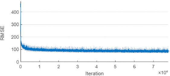
Training progress of the LSTM through the RMSE indicator.

Fig. 6.

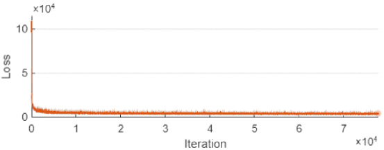
Training progress of the LSTM through the Loss indicator.

The RMSE is calculated according to the formula $\text{RMSE}=\sqrt{\frac{\sum _{i=1}^{N}(y_{i}-{\hat{y}}_{i})^{2}}{N}}$ where N is the number of responses, y_i is the target output, and ${\hat{y}}_{i}$ is the model’s prediction for response i. The Loss is calculated as $Loss=\frac{1}{2S}\sum _{i=1}^{S}\sum _{j=1}^{N}(y_{ij}-{\hat{y}}_{ij})^{2}$ , where S is the sequence length. In our case S = 96.

The values of both indicators are influenced by the numerical value of individual outputs, which exemplarily assume binary values of 1 or 10. Low conductance (value 1) is determined by dry areas, and high (value 10) by wet areas. Undoubtedly, both graphs’ regular, hyperbolic shapes are a testimony to the correct course of learning and a prediction of no overfitting. A network trained in this way should have the ability to generalise the tomographic problems.

2.5. The pixel-oriented ensemble (POE) concept

The POE concept is oriented towards selecting a model that generates a response based on the measurement vector and the pixel number in the image. In the case under consideration, the measurement vector consists of 96 values that are different for each measurement case. Earlier studies have shown that depending on the measurement vector, individual pixels should be predicted using different models because the differences in the measurement vector result in a preference for different machine learning methods. In the case discussed here, the classification model selects a method from the three available (previously trained) methods: ANN, LR, and LSTM.

The key here is to train the classification model. For this purpose, three response matrices were generated for 1000 randomly selected observations. Each matrix has a dimension of 1000 × 4955. Then, using the known patterns from the simulation set, the deviations for each pixel from 1000 observations were calculated, and the method (category) characterised by the minimum deviation was selected. Figure 7 shows the general workflow of the pixel-oriented ensemble (POE) method. In this way, the training set for the classification neural network was created, with 96 regression inputs and 3 output classes. For example, class 1 indicated a preference for AR, class 2 – LR, and class 3 – LSTM. Finally, the data prepared in this way was used to train the classification model of the neural network. As a result, the accuracy level of the classification model has reached 92%. In Fig. 7, Method I (OR) means the shallow neural network trained for classification.

Fig. 7.

The general principle of the pixel-oriented ensemble (POE) method.

The POE method is composed in such a way as to use the best reconstructions for specific pixels based on specific measurement vectors, choosing from several homogeneous methods. In our case, there are three homogeneous methods: ANN, LR and LSTM. All three homogeneous methods were trained on the same training set. In addition, the LSTM was trained using even more training cases by attaching the validation set to the training set. Therefore, in order to train the classifier (ANN classification network), the task of which is to select one of the three homogeneous methods (ANN, LR or LSTM) for a specific measurement vector (96 inputs) and each of the 4955 pixels of the image, a special training set had to be prepared. The inputs to this training set were the same measurement vectors used to train homogeneous regression models (ANN, LR and LSTM).

On the other hand, the output was classified and indicated one of the three methods (ANN, LR or LSTM), optimal for a given case and pixel (i.e. it generated the best result among all three homogeneous methods). In order to prepare such a classification training set, it was first necessary to obtain the results of the reconstruction for all cases included in the training set, using all three homogeneous methods. For example, if the training set for the classification model was 1000 cases, the output image’s resolution is 4955 pixels, and the number of homogeneous methods included in the POE is 3. Preparing the training set for the ANN classifier requires 14,865,000 (1000 observations × 3 methods × image resolution 4955) reconstruction. With such data, you can compare the results for 1000 measurements and choose the best (out of 3) method for every 4955 pixels, thus creating a training set for the classification model.

Figure 8 shows the preparation process and operation of the POE method.

Fig. 8.

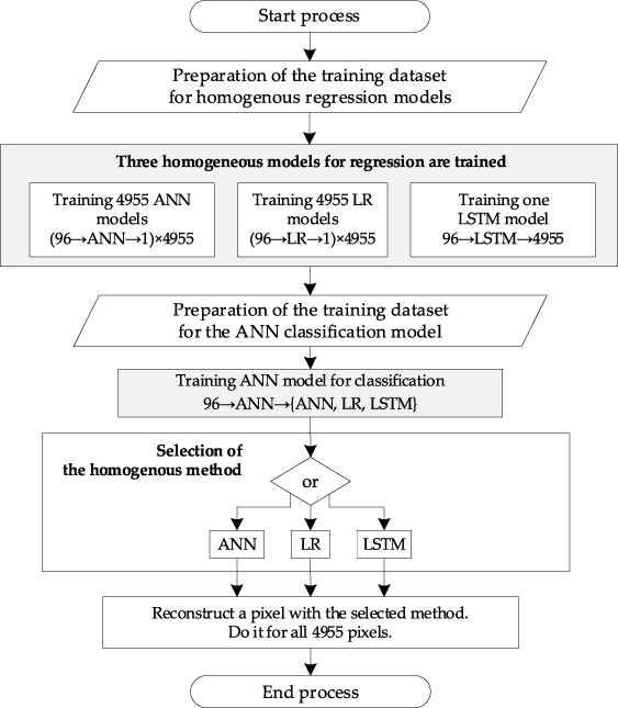
The flowchart of new concept (POE) modelling.

Figure 9 shows the proportional number of choices of individual methods for individual pixels in the context of 1000 random measurement cases. The most frequently used method was ANN (52%). LSTM (41%) was in second place. The least frequently chosen method was LR (7%).

Fig. 9.

The proportions of the classification of homogeneous methods within the POE concept for 1000 randomly selected measurement cases.

3. Results and discussion

In order to objectively compare the four methods, 4 commonly used criteria/indicators were used: root mean square error (RMSE), normalised mean square error (NMSE), relative image error (RIE), and image correlation coefficient (ICC). The RMSE formula has already been given. NMSE is calculated according to the formula $\text{NMSE}=\frac{\Vert \boldsymbol{y}-\hat{\boldsymbol{y}}\Vert ^{2}}{\Vert \boldsymbol{y}-\overline{\boldsymbol{y}}\Vert ^{2}}$ , where ∥⋅∥ is the L2–norm vector [35]. RIE is satisfied by $\text{RIE}=\frac{\Vert \boldsymbol{y}-\hat{\boldsymbol{y}}\Vert }{\Vert \boldsymbol{y}\Vert }$ and $\text{ICC}=\frac{\sum _{i=1}^{n}(y_{i}-\overline{\boldsymbol{y}})({\hat{y}}_{i}-\overline{\hat{\boldsymbol{y}}})}{\sqrt{\sum _{i=1}^{n}(y_{i}-\overline{\boldsymbol{y}})^{2}\sum _{i=1}^{n}({\hat{y}}_{i}-\overline{\hat{\boldsymbol{y}}})^{2}}}$ , where $\overline{\hat{\boldsymbol{y}}}$ is the mean of the model’s prediction for response i. The smaller the RMSE, NMSE, and RIE, the better. The ICC is the better, the closer to 1, the worse, and the closer m is to zero. Table 2 compares the 3 methods of ANN, LR, LSTM and POE. For this purpose, four criteria have been defined as indicators: RMSE, NMSE, RIE and ICC. 1000 randomly selected cases of moisture were assessed. As can see, in all cases, the best results were obtained using the POE method. It should be objectively stated that some of the differences are very small. For example, the NMSE comparison for LSTM is 0.008 and POE is 0.005. The ICC for LSTM is 0.825, and for POE, it is 0.836. On the other hand, the RMSE for LR is as high as 6,597, which is a big difference.

Table 2
Reconstruction quality indicators for individual methods

Indicator Methods of reconstruction

ANN LR LSTM POE

RMSE 1.720 6.597 0.978 0.631

NMSE 0.013 0.056 0.008 0.005

RIE 0.188 0.405 0.157 0.126

ICC 0.808 0.622 0.825 0.836

Indicator	Methods of reconstruction
RMSE	1.720	6.597	0.978	0.631
NMSE	0.013	0.056	0.008	0.005
RIE	0.188	0.405	0.157	0.126
ICC	0.808	0.622	0.825	0.836

Figure 10 compares 3D reconstructions obtained with ANN, LR, LSTM and POE methods. Three different cases of a damp wall were selected for the method comparison. In the first line of the figure, there are reference images (patterns). The following lines contain reconstructions made using ANN, LR, LSTM methods and the new POE concept.

Fig. 10.

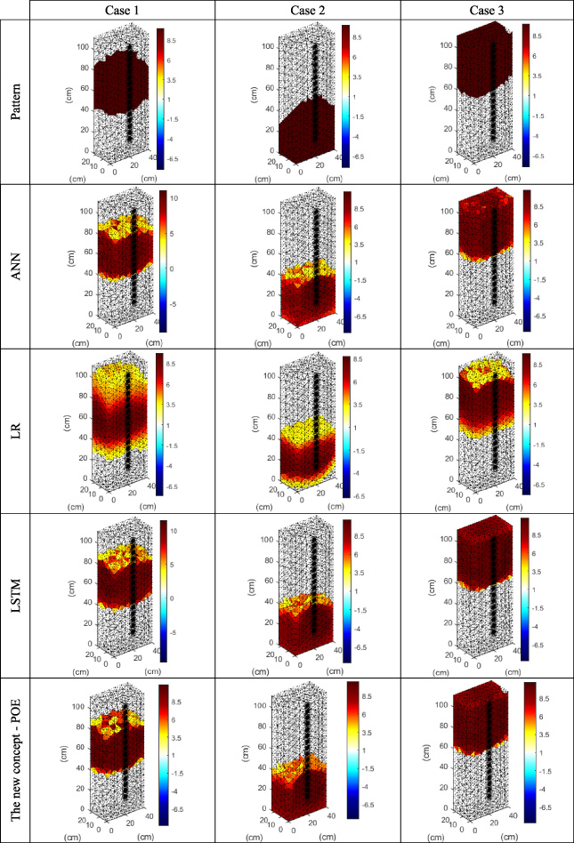
Comparison of 3D reconstructions obtained with ANN, LR, LSTM and POE methods.

The visual comparison is not prescriptive and burdened with the bias of subjective assessment, but it is visible that the LR reconstructions are worse than the others. In the case of ANN and LSTM methods, the differences are less noticeable and less obvious.

4. Conclusions

The article presents the concept of using a hybrid machine learning method, which guarantees better results than any of the homogeneous methods included in the pixel-oriented ensemble (POE) system thanks to training many models. The concept was applied to imaging the moisture inside a brick wall by solving the inverse problem in electrical impedance tomography. The high quality of the reconstruction was confirmed by comparing the images generated by the three components (homogeneous) methods of ANN, LR and LSTM and POE. All the methods presented, including POE, enable spatial visualisation of the moisture distribution inside the wall. It is a fundamental difference compared to the classical methods that test the humidity only at selected wall points. The comparison of error indicators and personal observation confirmed the high effectiveness of the new concept. Future research will focus on sequencing the moisture expansion processes inside porous materials, which will increase the effectiveness of tomographic methods.

References

Hoła

, Methodology for the in situ testing of the moisture content of brick walls: An example of application, Arch. Civ. Mech. Eng.20(4) (2020), 3, doi:10.1007/s43452-020-00120-3.

Rymarczyk

, Comparison of machine learning methods in electrical tomography for detecting moisture in building walls, Energies14(10) (2021), 2777, doi:10.3390/en14102777.

Rymarczyk

Kłosowski

and Kozłowski

, A non-destructive system based on electrical tomography and machine learning to analyse the moisture of buildings, Sensors18(7) (2018), 2285, doi:10.3390/S18072285.

Hola

, Measuring of the moisture content in brick walls of historical buildings-the overview of methods, IOP Conf. Ser.: Mater. Sci. Eng.251(1) (2017), doi:10.1088/1757-899X/251/1/012067.

Udawattha

C.D.

Galkanda

G.A.H.H.

and Halwatura

R.U.

, A study on natural rain surface erosion of different walling materials in tropics, in: MERCon 2018 – 4th Int. Multidiscip. Moratuwa Eng. Res. Conf., 2018, pp. 84–89. doi:10.1109/MERCON.2018.8421938.

Dusek

and Mikulka

, Measurement-based domain parameter optimisation in electrical impedance tomography imaging, Sensors21(7) (2021), 2507, doi:10.3390/S21072507.

Hoła

Matkowski

and Hoła

, Analysis of the moisture content of masonry walls in historical buildings using the basement of a medieval town hall as an example, Proc. Eng.172 (2017), 363–368, doi:10.1016/j.proeng.2017.02.041.

Babout

Grudzień

Wiącek

Niedostatkiewicz

Karpiński

and Szkodo

, Selection of material for X-ray tomography analysis and DEM simulations: Comparison between granular materials of biological and non-biological origins, Granul. Matter.20(3) (2018), 38, doi:10.1007/s10035-018-0809-y.

Banasiak

, Study on two-phase flow regime visualisation and identification using 3D electrical capacitance tomography and fuzzy-logic classification, Int. J. Multiph. Flow58 (2014), 1–1410.1016/J.IJMULTIPHASEFLOW.2013.07.003.

10.

Garbaa

Jackowska-Strumiłło

Grudzień

and Romanowski

, Application of electrical capacitance tomography and artificial neural networks to rapid estimation of cylindrical shape parameters of industrial flow structure, Arch. Electr. Eng.65(4) (2016), 657–669, doi:10.1515/aee-2016-0046.

11.

Kryszyn

and Smolik

, Toolbox for 3D modelling and image reconstruction in electrical capacitance tomography, Inform. Control Meas. Econ. Environ. Prot.7(1) (2017), 137–145, doi:10.5604/01.3001.0010.4603.

12.

Kryszyn

Wanta

D.M.

and Smolik

W.T.

, Gain adjustment for signal-to-noise ratio improvement in electrical capacitance tomography system EVT4, IEEE Sens. J.17(24) (2017), 8107–8116, doi:10.1109/JSEN.2017.2744985.

13.

Majchrowicz

Kapusta

Jackowska-Strumiłło

and Sankowski

, Acceleration of image reconstruction process in the electrical capacitance tomography 3D in heterogeneous, multi-GPU system, Inform. Control Meas. Econ. Environ. Prot.7(1) (2017), 37–41, doi:10.5604/01.3001.0010.4579.

14.

Wajman

, Metrological evaluation of a 3D electrical capacitance tomography measurement system for two-phase flow fraction determination, Meas. Sci. Technol.24(6) (2013), 065302, doi:10.1088/0957-0233/24/6/065302.

15.

Duraj

Korzeniewska

and Krawczyk

, Classification algorithms to identify changes in resistance, Prz. Elektrotech.1(12) (2015), 82–84, doi:10.15199/48.2015.12.19.

16.

Szczesny

and Korzeniewska

, Selection of the method for the earthing resistance measurement, Prz. Elektrotech.94(12) (2018), 178–181.

17.

Rymarczyk

Kłosowski

Tchórzewski

Cieplak

and Kozłowski

, Area monitoring using the ERT method with multisensor electrodes, Prz. Elektrotech.95(1) (2019), 153–156.

18.

Shanghai

Study on reconstruction algorithm of x-ray fluorescence computed tomography based on L1/2-norm and expectation-maximum, in: 2021 19th International Conference on Optical Communications and Networks (ICOCN), 2021, pp. 1–3. doi:10.1109/ICOCN53177.2021.9563774.

19.

Kozlowski

Rymarczyk

and Klosowski

, , Logistic regression application to image reconstruction in UST, 2019. doi:10.23919/PTZE.2019.8781722.

20.

Mikulka

, GPU-accelerated reconstruction of T2 maps in magnetic resonance imaging, Meas. Sci. Rev.15(4) (2015), 210–218, doi:10.1515/msr-2015-0029.

21.

Krawczyk

and Korzeniewska

, Magnetophosphenes – history and contemporary implications, Prz. Elektrotech.1(1) (2018), 63–66, doi:10.15199/48.2018.01.16.

22.

Soleimani

Adler

Dai

and Peyton

A.J.

, Application of a single step temporal imaging of magnetic induction tomography for metal flow visualisation, Insight Non-Destruct. Test. Cond. Monit.50(1) (2008), 25–29. doi:10.1784/insi.2008.50.1.25.

23.

Korzeniewska

Sekulska-Nalewajko

Gocławski

Dróżdż

and Kiełbasa

, Analysis of changes in fruit tissue after the pulsed electric field treatment using optical coherence tomography, Eur. Phys. J. Appl. Phys.91(3) (2020), 30902. doi:10.1051/EPJAP/2020200021.

24.

Kabanikhin

S.I.

, Definitions and examples of inverse and ill-posed problems, J. Inverse Ill-Posed Probl.16(4) (2008), 317–357, doi:10.1515/JIIP.2008.019.

25.

Liu

Jia

Zhang

Y.D.

and Yang

, Image reconstruction in electrical impedance tomography based on structure-aware sparse bayesian learning, IEEE Trans. Med. Imaging37(9) (2018), 2090–2102, doi:10.1109/TMI.2018.2816739.

26.

Rymarczyk

, Historical buildings dampness analysis using electrical tomography and machine learning algorithms, Energies14(5) (2021), 1307, doi:10.3390/en14051307.

27.

Liu

Zhao

Khambampati

Seppänen

A.K.

and Du

, A parametric level set method for imaging multiphase conductivity using electrical impedance tomography, IEEE Trans. Comput. Imaging, Comput. Imaging, IEEE Trans. on, IEEE Trans. Comput. Imaging4(4) (2018), 552, doi:10.1109/TCI.2018.2863038.

28.

Rymarczyk

Kozłowski

Tchórzewski

Kłosowski

and Adamkiewicz

, Applying the logistic regression in electrical impedance tomography to analyze conductivity of the examined objects, Int. J. Appl. Electromagn. Mech.64(S1) (2020), doi:10.3233/JAE-209520.

29.

Liu

Huang

Yang

and Jia

, Accelerated structure-aware sparse bayesian learning for three-dimensional electrical impedance tomography, IEEE Trans. Ind. Inform.15(9) (2019), 5033–5041, doi:10.1109/tii.2019.2895469.

30.

Liu

Huang

Tan

and Jia

, Efficient multitask structure-aware sparse bayesian learning for frequency-difference electrical impedance tomography, IEEE Trans. Ind. Inform.17(1) (2021), 463–472, doi:10.1109/TII.2020.2965202.

31.

Kupis

S.R.

, , Methods for the electrical impedance tomography inverse problem: deep learning and regularization with wavelets. All Theses. 3543, Clemson University, 2021. https://tigerprints.clemson.edu/all_theses/3543.

32.

Adler

and Lionheart

W.R.B.

, Uses and abuses of EIDORS: An extensible software base for EIT, Physiol. Meas.27(5) (2006), S25–S42, doi:10.1088/0967-3334/27/5/S03.

33.

Porzuczek

, Assessment of the spatial distribution of moisture content in granular material using electrical impedance tomography, Sensors19(12) (2019), 2807, doi:10.3390/s19122807.

34.

Kłosowski

Rymarczyk

Wójcik

Skowron

Cieplak

and Adamkiewicz

, The use of time-frequency moments as inputs of LSTM network for ECG signal classification, Electronics9(9) (2020), 1452, doi:10.3390/electronics9091452.

35.

Fabijańska

and Banasiak

, Graph convolutional networks for enhanced resolution 3D electrical capacitance tomography image reconstruction, Appl. Soft Comput.110 (2021), 107608, doi:10.1016/J.ASOC.2021.107608.

Indicator	Methods of reconstruction
	ANN	LR	LSTM	POE
RMSE	1.720	6.597	0.978	0.631
NMSE	0.013	0.056	0.008	0.005
RIE	0.188	0.405	0.157	0.126
ICC	0.808	0.622	0.825	0.836

Identification of moisture inside walls in buildings using machine learning and ensemble methods

Abstract

Keywords

1. Introduction

2. Materials and methods

2.1. Data preparation and validation

Table 2 Reconstruction quality indicators for individual methods Indicator Methods of reconstruction ANN LR LSTM POE RMSE 1.720 6.597 0.978 0.631 NMSE 0.013 0.056 0.008 0.005 RIE 0.188 0.405 0.157 0.126 ICC 0.808 0.622 0.825 0.836

References

Table 2
Reconstruction quality indicators for individual methods

Indicator Methods of reconstruction

ANN LR LSTM POE

RMSE 1.720 6.597 0.978 0.631

NMSE 0.013 0.056 0.008 0.005

RIE 0.188 0.405 0.157 0.126

ICC 0.808 0.622 0.825 0.836