Magnetic force prediction of hybrid magnet with Halbach array using generalized regression neural network optimized by a modified aquila optimizer

Abstract

This paper addresses the balancing of global and local searches in the recently proposed AO (Aquila Optimizer) algorithm. The original random algorithm is modified using normal-distribution parameters, and an adaptive function represented by a Weibull function is added to the motion law of the predator. Sixteen benchmark functions are used to test the improved algorithm against several recently developed algorithms. The results show that the accuracy and convergence speed of the modified algorithm are improved while the advantages of the original algorithm are retained. In solving the problems of a complex calculation and limited solution in the design of a hybrid electromagnetic structure based on a Halbach array, a prediction model based on the improved algorithm and generalized regression neural network (GRNN) is designed for improved prediction accuracy of the GRNN. Thirty groups of data are obtained using Ansoft, and the prediction accuracy of the improved GRNN is verified using the data. The mean squared error (MSE) of normalized prediction results reaches 0.1404. The improved prediction model has the prediction error less than 10% and its performance is better than the RBF and the KCV-GRNN.

1. Introduction

Optimization is a common problem in engineering whereby better results are obtained on the existing basis adopting certain processes and methods. Common optimization problems can be divided into linear, non-linear, single-objective, and multi-objective problems. Optimization algorithms are used to solve complex problems. And many algorithms have recently been proposed, broadening the application fields of algorithms [1].

The meta-heuristic (MH) algorithm [2] is the main research object of this study. Meta-heuristic algorithms are mainly divided into four types, the first being the swarm intelligence (SI) algorithm. The swarm intelligence algorithm applies the process of swarm optimization to computational optimization, and the most common algorithm of this type are particle swarm optimization (PSO) [3], artificial bee colony (ABC) [4], and ant colony optimization (ACO) [5]. The relatively new algorithms in the field of swarm intelligence include the bonobo optimizer (BO) [6] and aquila optimizer (AO) [7].

The second is the evolutionary algorithm (EA) that is based on imitating biological evolution to achieve optimization. The most common algorithms of this type are genetic algorithms (GA) [8] and differential evolution (DE) [9]. However, relatively new algorithms in the field of evolutionary algorithms include the invasive tumor growth optimization algorithm (ITGO) [10].

The third is a physics-based algorithm (PHA) that realizes optimization by simulating the laws of physics. The gravitational search algorithm (GSA) [11] is more common and is optimized by simulating the action law of gravity. However, relatively new physics-based algorithms include central force optimization (CFO) [12].

The last is a human-based algorithm (HBA) that computes based on human optimization behavior. Common algorithms in machine learning are teaching and learning-based optimization (TLBO) [13] and reinforcement learning algorithms (Q-learning [14], SARSA [15]), which mainly imitate human education and learning behavior. The relatively new algorithms in the field of human-based algorithms include the future search algorithm (FSA) [16] and deep Q-network (DQN) [17].

Although there are different types of algorithm, they have a common running process of a global development and a local search. The main task of global development is improving the convergence speed by preliminarily determining the range of optimal values. The main task of the local search is ensuring convergence accuracy by obtaining optimal results within the range of optimal values. The reasonable setting of the global search stage and the local search stage considering the balance between accuracy and speed.

At the same time, the main task of the algorithm is solving the optimization problem. It is best to use different optimization algorithms for different optimization problems. When the optimization problem is more complex or takes a long time to solve, the balance of the algorithm itself will need to be adjusted. An algorithm that places emphasis on the local search is suitable for a problem whose solution range is easy to determine, whereas the algorithm that places emphasis on the global search is suitable for a problem whose solution accuracy does not need to be high. The adaptive algorithm can adjust the balance as the characteristics of the problem change in the process of solving.

In summary, algorithms with different degrees of balance are generally required to solve diverse optimization problems. At present, there are two ways to solve a problem. One is to find a better algorithm to solve the problem and the other is to solve the problem by improving the algorithm. This paper mainly discusses the second method. As the optimization problem, this paper chooses the electromagnetic structural design of a Halbach hybrid array for application.

Maglev technology has been widely used in maglev bearing [18–23], train [24–26], and control platform [27–32], and so on. An electromagnetic actuator is the main mechanical structure that suspends objects in a contactless manner in a maglev system, and comprises a mix of electromagnets, permanent magnets, and electromagnetic permanent magnets. In an electromagnetic permanent-magnet hybrid structure, the permanent-magnet structure provides the main support force and the electromagnetic structure provides auxiliary control. A hybrid electromagnetic permanent-magnet structure represented by a Halbach array has been studied for its magnetic enhancement effect.

Owing to the physical coupling between the electromagnetic field and the structure, the relationship between the magnetic force variation in the permanent magnet-electromagnetic hybrid structure and the structural parameters shows a non-linear and strong coupling phenomenon, which adds complexity to the overall design of the structure. To solve these problems, researchers have proposed theoretical solutions [33–37], a simulation analysis [38], a combination of theory and finite elements [39], and experimental research [40,41]. The Halbach model was based on the accurate solution of Laplace’s and Poisson’s partial differential equations (PDEs) using a variable-separation method [34]. However, the model solution of the Halbach array has some errors and limitations, and the SVM-GS model adopted by Li et al. provides research ideas [42].

With the development of neural networks, artificial intelligence has been adopted to solve design problems in the maglev field [43–48]. In contrast with traditional numerical simulations, the neural network methodology adopts a training data set to obtain a law of the data input and output, thus avoiding the complexity of the actual structure in practical application design, establishing a structure prediction model, and achieving higher calculation accuracy. As a radial neural network, the Generalized Regression Neural Network (GRNN) obtains a better prediction model on the premise of training on a small sample dataset [49–51]. In [50], the K-folder cross validation (K-CV) was used to improve the generalized regression neural network (GRNN) to model and predict the lamellar spacing and mechanical properties of hypereutectoid steels with a small sample data. If an optimization algorithm is used to optimize the influencing parameters of the network structure, the accuracy of the prediction model can be greatly improved, providing convenience in the actual design of electromagnetic structures and shortening the design cycle [52–55].

The aquila optimizer (AO) algorithm has excellent algorithmic performance and has a wide range of applications, including neural networks and big data. The performance of the AO algorithm can be improved by introducing Lévy flight, interruptions, mutations, and other random components (relating to either local or global search methods) [7]. The present paper proposes a prediction model of a modified AO algorithm combined with the GRNN, applies the prediction model in the prediction of the electromagnetic force of a Halbach hybrid array, and verifies the effectiveness and feasibility of the prediction model by using test functions and conducting simulation experiments.

2. AO algorithm

This paper mainly discusses a new swarm intelligence algorithm, namely the AO algorithm [7]. The algorithm mimics the hunting behavior of a bird of the genus Aquila. In nature, the hunting process of Aquila can be divided into the following steps.

Aquila hovers in the sky. When they first find their prey, Aquila glide close to the prey.

Prey that senses the approach of Aquila will run away, but Aquila do not attack rashly. Instead, Aquila track the prey through changes in flight altitude and distance.

Aquila wait until the tracking distance is sufficiently short. When the distance reduces to a certain threshold, Aquila attack their prey.

Aquila confirm the capture, completing the capturing process.

Therefore, compared with other meta-heuristic algorithms, the Aquila hunt has four main characteristics. First, Aquila do not hunt blindly. From the beginning to the end of the hunt, Aquila spend the first two-thirds of their time searching and determining the approximate range of their prey. In the remaining one-third of the capture time, Aquila make more precise captures in the general area. During the two periods, Aquila hunt in manner similar to global development and then a local search. From the point of view of the algorithm, this search method avoids Aquila falling into a local optimum, and the Aquila flying pursuit method based on Lévy flight enhances the global development of the algorithm. The running process of the specific algorithm can be divided into four stages. The first stage is the beginning stage of the algorithm, and the initial solution of the algorithm is obtained through Eq. (1). $\begin{eqnarray}\displaystyle x_{i,j}=(\mathit{UB}_{j}-\mathit{LB}_{j})\times \mathit{rand}+\mathit{LB}_{j}. & & \displaystyle\end{eqnarray}$ (1)

x _{i, j} in the equation is a value in the candidate solution X of the algorithm, and the correlation is expressed by Eq. (2). The solution was randomly generated between the upper bound (UB) and the lower bound (LB) of a given parameter. LB _j denotes to the jth lower bound, and UB _j denotes to the jth upper bound of the given problem. The rand represents a value randomly generated between 0 and 1. $\begin{eqnarray}\displaystyle X=\left[\begin{array}{@{}cccc@{}}x_{1,1} & x_{1,2} & \cdots ∼ & x_{1,\text{dim}}\\ x_{2,1} & x_{2,2} & \cdots ∼ & x_{2,\text{dim}}\\ \vdots & \vdots & \ddots & \vdots \\ x_{N,1} & x_{N,2} & \cdots ∼ & x_{N,\text{dim}}\end{array}\right]. & & \displaystyle\end{eqnarray}$ (2)

It can also be observed from the equation that i (i = 1, 2, 3, … , N) and j (j = 1, 2, 3, … , dim) determine the position of x _{i, j} in X. N, dim is the parameter of the algorithm population, where N is the population number of candidate solutions of the algorithm, and dim represents the dimension of the solution. Based on whether the iteration number of the algorithm is within the first two-thirds of the total number of iterations, the operation process of the algorithm is divided into the second and third stages. When the number of algorithm iterations is in the first two-thirds, that is, in the second stage, the algorithm equation is as follows: $\begin{eqnarray}\displaystyle \text{} & \text{} & \displaystyle X_{1}^{t+1}=X_{\text{best}}^{t}\times \left(1-\frac{t}{T}\right)+(X_{M}^{t}-X_{\text{best}}^{t}\ast \mathit{rand})\end{eqnarray}$ (3) $\begin{eqnarray}\displaystyle \text{} & \text{} & \displaystyle X_{2}^{t+1}=X_{\text{best}}^{t}\times \text{Levy}(D)+X_{R}^{t}+(y-x)\ast \mathit{rand}\end{eqnarray}$ (4) where, $X_{1}^{t+1}$ and $X_{2}^{t+1}$ are the solutions of the next iteration of t, generated by the two search methods. This method is mathematically presented in Eqs (3) and (4). $X_{\text{best}}^{t}$ represents the best solution obtained by the algorithm before the tth iteration. $X_{M}^{t}$ represents the average value of the algorithm solution at the tth iteration, which can be expressed by Eq. (5). T represents the maximum number of algorithm iterations, which is the total number of algorithm iterations. t represents the current number of algorithm iterations. D is the dimension space, Levy(D) is the Levy flight distribution function, which is obtained using Eq. (6). $X_{R}^{t}$ is a random solution obtained in the range [1 N] at the tth iteration, while y and x are calculated using Eqs (8) and (9), respectively. $\begin{eqnarray}\displaystyle \text{} & \text{} & \displaystyle \displaystyle X_{M}^{t}=\frac{1}{N}\mathop{\sum }_{i=1}^{N}X_{i}^{t}\end{eqnarray}$ (5) $\begin{eqnarray}\displaystyle \text{} & \text{} & \displaystyle \displaystyle \text{Levy}(D)=0.01\times \frac{\mathit{rand}\ast {\delta}}{(\mathit{rand})^{\frac{1}{{\beta}}}}.\end{eqnarray}$ (6)

δ is calculated using Eq. (7): $\begin{eqnarray}\displaystyle \displaystyle {\delta}=\left(\frac{{\Gamma}(1+{\beta})\times \sin \left({\displaystyle \frac{{\pi}{\beta}}{2}}\right)}{{\Gamma}\left({\displaystyle \frac{1+{\beta}}{2}}\right)\times {\beta}\times 2^{\left(\frac{{\beta}-1}{2}\right)}}\right). & & \displaystyle\end{eqnarray}$ (7)

𝛽 is the parameter value set in the equation. In this paper and subsequent improvements, the setting was the same as that of the original algorithm, and the value size was 1.5. $\begin{eqnarray}\displaystyle \text{} & \text{} & \displaystyle y=(r_{1}+0.00565\times D_{1})\times \cos \left(-0.005\times D_{1}+\frac{3}{2}{\pi}\right)\end{eqnarray}$ (8) $\begin{eqnarray}\displaystyle \text{} & \text{} & \displaystyle x=(r_{1}+0.00565\times D_{1})\times \sin \left(-0.005\times D_{1}+\frac{3}{2}{\pi}\right)\end{eqnarray}$ (9) where, r ₁ takes a value between 1 and 20. Referring to the parameter setting of the original algorithm, the value of r ₁ is set to 10. D ₁ is an integer from one to the length of the search space (dim).

In the third stage, the AO algorithm was based on the dynamic approach process of the distance between the Aquila and the prey. The prey exhibited a random escape mode. The Aquila pursued the prey faster with the progress of capture according to the operation mode of the prey. While approaching, the Aquila uses Levy flight for the capture, ensuring that the algorithm improves the capture accuracy and reduces the error rate of the Aquila. The relevant equations are as follows: $\begin{eqnarray}\displaystyle \text{} & \text{} & \displaystyle X_{3}^{t+1}=(X_{\text{best}}^{t}-X_{M}^{t})\times {\alpha}-\mathit{rand}+((\mathit{UB}-\mathit{LB})\times \mathit{rand}+\mathit{LB})\times {\delta}\end{eqnarray}$ (10) $\begin{eqnarray}\displaystyle \text{} & \text{} & \displaystyle X_{4}^{t+1}=\mathit{QF}(t)\times X_{\text{best}}^{t}-(G_{1}\times X^{t}\times \mathit{rand})-G_{2}\times \text{Levy}(D)+\mathit{rand}\times G_{1}\end{eqnarray}$ (11) where, $X_{3}^{t+1}$ and $X_{4}^{t+1}$ are the solutions of the next iteration of t, generated by the two search methods. This method is mathematically presented in Eqs (10) and (11). 𝛼 adjusts the parameters for the search in the algorithm, which is consistent with the author’s reference value, fixed to 0.1. G ₁ and G ₂ and QF (t) were obtained by Eqs (12), (13) and (14). $\begin{eqnarray}\displaystyle \text{} & \text{} & \displaystyle \displaystyle G_{1}=2\times \mathit{rand}-1\end{eqnarray}$ (12) $\begin{eqnarray}\displaystyle \text{} & \text{} & \displaystyle \displaystyle G_{2}=2g=2\left(1-\frac{t}{T}\right)\end{eqnarray}$ (13) $\begin{eqnarray}\displaystyle \text{} & \text{} & \displaystyle \displaystyle \mathit{QF}(t)=t^{\frac{2\times \mathit{rand}-1}{(1-T)^{2}}}.\end{eqnarray}$ (14)

The change in QF can cause the distance between Aquila and prey to show a certain range of dynamic changes, which can avoid local optimization owing to very rapid convergence.

In the fourth stage, the algorithm obtains the optimal solution result and ends to obtain the final value. Based on the above, the basic flow of AO algorithm can be shown in Fig. 1. The fitness function value in the figure represents the value obtained by solving the fitness function of X.

Fig. 1.

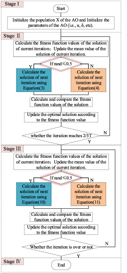
The basic flow of Aquila Optimizer.

3. Modified AO algorithm

The AO algorithm has been used in predicting oil production because of its excellent optimization performance [56]. At the same time, the author compares the AO algorithm with several other optimization algorithms and finds that the AO algorithm has certain advantages. The AO algorithm could thus be popularized and used in various fields to some extent, and we can further develop the optimization potential of the algorithm itself.

It is thus considered that the advantage of the AO algorithm is that the algorithm realizes optimization through Eq. (3) with certain dynamic adaptive changes. The algorithm uses random parameters to balance the global development and local search. We can further improve the advantages of the algorithm as described in the following.

3.1. Random-parameter modification

The AO algorithm mainly imitates the process of Aquila catching prey. Equations (3), (4), (10), and (11) show that the use of random parameters determines the change in distance between Aquila and prey and the balance of the algorithm development and search. When considering natural or engineering practical problems, we find that the emergence of an optimal value generally follows a certain rule of parameters, such as the golden ratio or a normal distribution. Among these rules, taking a random number from a normal distribution is a common method of algorithm parameter optimization, which improves the search accuracy and performance of the algorithm [57–64]. The present paper thus uses this law to modify the parameters randomly in the AO algorithm, so as to ensure accuracy of the algorithm and optimize the balance of the algorithm. Here, randn represents the random number taken from a normal distribution. Consequently, Equations (3), (4), (10), (11) become the following: $\begin{eqnarray}\displaystyle \text{} & \text{} & \displaystyle \displaystyle X_{1}^{t+1}=X_{\text{best}}^{t}\times \left(1-\frac{t}{T}\right)+(X_{M}^{t}-X_{\text{best}}^{t}\ast \mathit{randn})\end{eqnarray}$ (15) $\begin{eqnarray}\displaystyle \text{} & \text{} & \displaystyle \displaystyle X_{2}^{t+1}=X_{\text{best}}^{t}\times \text{Levy}(D)+X_{R}^{t}+(y-x)\ast \mathit{randn}\end{eqnarray}$ (16) $\begin{eqnarray}\displaystyle \text{} & \text{} & \displaystyle \displaystyle X_{3}^{t+1}=(X_{\text{best}}^{t}-X_{M}^{t})\times {\alpha}-\mathit{randn}+((\mathit{UB}-\mathit{LB})\times \mathit{randn}+\mathit{LB})\times {\delta}\end{eqnarray}$ (17) $\begin{eqnarray}\displaystyle \text{} & \text{} & \displaystyle \displaystyle X_{4}^{t+1}=\mathit{QF}(t)\times X_{\text{best}}^{t}-(G_{1}\times X^{t}\times \mathit{randn})-G_{2}\times \text{Levy}(D)+\mathit{randn}\times G_{1}\end{eqnarray}$ (18) $\begin{eqnarray}\displaystyle \text{} & \text{} & \displaystyle \displaystyle \mathit{QF}_{n}(t)=t^{\frac{2\times \mathit{randn}-1}{(1-T)^{2}}}.\end{eqnarray}$ (19)

Taking a random number from a normal distribution means that the generated random value follows a normal distribution in terms of probability, and the value range remains within [0, 1]. In the above equation, the addition of the normal-distribution random number can be understood as Aquila approaching a location at which the prey is more likely to appear in the process of catching prey. Additionally, Aquila will attack their prey when it is easy to catch the prey. The above improvement reduces the blindness of algorithm optimization and improves the search precision and speed of the algorithm to certain extents.

3.2. Enhanced adaptive range change

In the search process, Aquila constantly switch between global development and a local search, and changes in parameter values and variables will affect the running speed and accuracy of the algorithm. Adopting the time intervals used by Aquila, we divide the iteration of the AO algorithm into an early stage (two-thirds of the search time) and late stage (one-third of the search time). Through the division of the early and late stage, we hope that the AO algorithm conducts the global development as well as possible. Based on Eq. (13) and the principle of the algorithm, X can be viewed as the position of the Aquila in the algorithm’s search process, and X _best is denoted as the position of the prey. And $(1-\frac{t}{T})$ can be considered as the spacing of Aquila and prey. In the early stage of the algorithm, it is seen from Eq. (13) that with the advance of the iteration time, the effect of the optimal position gradually decreases, which corresponds to Aquila gradually approaching the area where the prey appears. The later stage of the algorithm, as shown in Eq. (13), corresponds to Aquila launching a fierce attack on their prey, and toward the end, Aquila gradually approach the prey and finally capture the prey. $\begin{eqnarray}\displaystyle g=1-\frac{t}{T}. & & \displaystyle\end{eqnarray}$ (20)

The g value decreases linearly with an increasing number of iterations, which means that the algorithm has the property of adaptive change to a certain extent. However, a basic linear change does not completely correspond to the nature of the change. The rate of change in the approaching degree should be consistent with a certain law for the physical energy to be allocated reasonably. This paper proposes that the variation law of g _w follows a Weibull function based on the iteration cycle change, with the range still satisfying the variation range of Eq. (13). g _w is calculated using Eq. (22). $\begin{eqnarray}\displaystyle \text{} & \text{} & \displaystyle s(t)=\frac{{\beta}}{{\eta}}\left(\frac{t}{{\eta}}\right)^{{\beta}-1}\text{e}^{-(\frac{t}{{\eta}})^{{\beta}}}\end{eqnarray}$ (21) $\begin{eqnarray}\displaystyle \text{} & \text{} & \displaystyle g_{w}(t)=\int _{1}^{t}Ss(t)∼\text{d}t.\end{eqnarray}$ (22)

A Weibull function, as a probability distribution function, agrees with the expression of natural law. The neutralization of the equation and the fixed parameters (𝜂, 𝛽) of the Weibull function determine the variation and rule of the probability value generated using the Weibull function. This paper takes S as 1. So, if the fixed parameters of the Weibull function are properly adjusted, the Weibull function values can show nonlinear variations, as illustrated in Fig. 2. The Weibull function value is widely used in related fields for this characteristic trend [65–72]. Equation (15) is thus rewritten as the following Eq. (23). $\begin{eqnarray}\displaystyle X_{1}^{t+1}=X_{\text{best}}^{t}\times g_{w}(t)+(X_{M}(t)-X_{\text{best}}(t)\ast \mathit{randn}). & & \displaystyle\end{eqnarray}$ (23)

It is concluded from the characteristics of the Weibull function that in each iteration, the situation of Aquila themselves being close to the optimal value will change. A slower change in the g value increases the chance of observation. When Aquila approach the optimal value, the increase in the change speed accelerates the operation and search speed, such that there is an adaptive law of searching for the optimal value. On the basis of the corresponding adaptive distribution model, the balance of the global development and local search of the AO algorithm is improved.

Fig. 2.

The comparison of g values.

3.3. Faster adaptive hunting

Through the addition of the Weibull function, the algorithm has a good balance between the global development and local search in the second and third stages. However, in the third stage, when Aquila are close to the final result, there tends to be faster convergence. Therefore, the original linearly varying G ₂ is still used at this time, but an adaptive speed factor is added to accelerate convergence. To improve the hunting efficiency of Aquila during the final hunting period after full global development, this paper proposes adding an adaptive speed factor to Eq. (11) by referring to the particle swarm optimization algorithm. The equation is as follows: $\begin{eqnarray}\displaystyle v(t)=\arctan \left(\frac{t}{T}+\frac{1}{t}\right)+1. & & \displaystyle\end{eqnarray}$ (24)

Therefore, Equation (18) is transformed into the following: $\begin{eqnarray}\displaystyle X_{4}^{t+1}=\mathit{QF}(t)\times X_{\text{best}}^{t}-(G_{1}\times X^{t}\times \mathit{randn})-G_{2}\times \text{Levy}(D)\times v(t)+\mathit{randn}\times G_{1}. & & \displaystyle\end{eqnarray}$ (25)

Unlike the change in the Section 3.2, the change rule of the adaptive speed factor will increase with increase in time and the capture speed of the Aquila will improve in the later capture.

4. Evaluation of algorithm performance

To verify the performance of the improved adaptive AO, the improved algorithm and the original algorithm adopted the performance parameters set in this study. The difference is that in the improved adaptive algorithm, in addition to setting the performance parameters, the values of the Weibull function parameters are set as 𝜂 = 230 and 𝛽 = 3. The benchmark functions used in the tests are listed in Table 1. Emulation software MATLABR2018a was selected and operated on a computer with an operating system of Win10pro, a CPU of Intel^®core (TM) i5-4200H CPU@2.80 GHZ, 2794 MHZ.

Table 1
Algorithms used for comparative analysis and their population settings. NFEs denotes the number of objective function evaluations

Algorithm Population size NFEs

AO 30 30000

Modified AO 30 30000

WHO 30 30000

ACO 30 30000

PSO 30 30000

Algorithm	Population size	NFEs
AO	30	30000
Modified AO	30	30000
WHO	30	30000
ACO	30	30000
PSO	30	30000

To verify the superiority of the improved algorithm, we adopted some recently proposed algorithms. The benchmark functions are presented in Table 2. The algorithms used include the WHO [73], ACO [74], PSO [3], and the original AO. To ensure that each algorithm can show the corresponding excellent performance, the parameters adopted by the algorithm were subjected to the corresponding algorithm recommended by the author. Considering the importance of the population and iteration, the adopted population number is also based on the author’s suggested value. However, because a reasonable reference value has not been found for the population parameter values of some algorithms, to ensure the fairness of each algorithm in the operation, this section directly sets the NFEs (Number of Function Evaluations) value of each algorithm to 30 000 and the population number to 30. The results for each algorithm are presented in Table 3. f _min denotes the optimal value of the benchmark function.

Table 2

Standard benchmark functions used in this study

Function	Attribute	Description	Dimensions (n)	Range	f _min
F1	Unimodal	$\displaystyle f(x)=\sum _{i=1}^{n}x_{i}^{2}$	30	[−100, 100]	0
F2	Unimodal	$\displaystyle f(x)=\sum _{i=1}^{n}\|x_{i}\|+\prod _{i=1}^{n}\|x_{i}\|$	30	[−10, 10]	0
F3	Unimodal	$\displaystyle f(x)=\sum _{i=1}^{d}\left(\sum _{j=1}^{i}x_{j}\right)^{2}$	30	[−100, 100]	0
F4	Unimodal	$\displaystyle f(x)=\max \{\|x_{i}\|,1\leq i\leq n\}$	30	[−100, 100]	0
F5	Unimodal	$\displaystyle f(x)=\sum _{i=1}^{n-1}[100(x_{i}^{2}-x_{i+1})^{2}+(1-x_{i})^{2}]$	30	[−30, 30]	0
F6	Multimodal	$\displaystyle f(x)=\sum _{i=1}^{n}(-x_{i}\sin (\sqrt{\|x_{i}\|}))$	30	[−500, 500]	−418.9828 × n
F7	Multimodal	$\displaystyle f(x)=\sum _{i=1}^{n}[x_{i}^{2}-∼10\cos (2{\pi}x_{i})+∼10]$	30	[−5.12, 5.12]	0
F8	Multimodal	$\displaystyle \begin{array}{@{}l@{}}\displaystyle f(x)=-20\exp \left(-0.2\sqrt{\frac{1}{n}\sum _{i=1}^{n}x_{i}^{2}}\right)\\ \quad \displaystyle -\exp \left(\frac{1}{n}\sum _{i=1}^{n}\cos (2{\pi}x_{i})\right)+20+e\end{array}$	30	[−32, 32]	0
F9	Multimodal	$\displaystyle f(x)=∼1+\frac{1}{4000}\sum _{i=1}^{n}x_{i}^{2}-\prod _{i=1}^{n}\cos \left(\frac{x_{i}}{\sqrt{i}}\right)$	30	[−600, 600]	0
F10	Multimodal	$\displaystyle \begin{array}{@{}l@{}}\displaystyle f(x)=\frac{{\pi}}{n}\{10\sin ^{2}({\pi}y_{1})\}\\ \displaystyle \quad +∼\sum _{i=1}^{n-1}(y_{i}-1)^{2} [1+10\sin ^{2}({\pi}y_{i+1})\\ \displaystyle \quad +∼\sum _{i=1}^{n}u(x_{i},10,100,4),\text{where}\\ \displaystyle \quad y_{i}=1+\frac{x_{i}+1}{4},\\ \displaystyle \quad u(x_{i},a,k,m)\left\{\begin{array}{@{}ll@{}}K(x_{i}-a)^{m}\quad & \text{if}∼x_{i}>a\\ 0\quad & -a\leq x_{i}\leq a\\ K(-x_{i}-a)^{m}\quad & -a\geq x_{i}\end{array}\right.\end{array}$	30	[−50, 50]	0

Table 2 (Continued).

Function	Attribute	Description	Dimensions (n)	Range	f _min
F11	Multimodal	$\displaystyle \begin{array}{@{}l@{}}\displaystyle f(x)=0.1(\sin ^{2}(3{\pi}x_{1})\\ \displaystyle \quad +∼\sum _{i=1}^{n}(x_{i}-1)^{2}[1+\sin ^{2}(3{\pi}x_{1})]\\ \displaystyle \quad +∼(x_{n}-1)^{2}1+\sin ^{2}(3{\pi}x_{n}))\\ \displaystyle \quad +∼\sum _{i=1}^{n}u(x_{i},5,100,4)\end{array}$	30	[−50, 50]	0
F12	Fixed-dimension	$\displaystyle f(x)=\left(\frac{1}{500}+\sum _{j=1}^{25}\frac{1}{j+\sum _{i=1}^{2}}(x_{i}-a_{ij})\right)^{-1}$	2	[−65, 65]	1
F13	Fixed-dimension	$\displaystyle \begin{array}{@{}l@{}}f(x)=4x_{1}^{2}-2.1x_{1}^{4}\\ \quad +∼\frac{1}{3}x_{1}^{6}+x_{1}x_{2}-4x_{2}^{2}+4x_{2}^{4}\end{array}$	2	[−5, 5]	−1.0316
F14	Fixed-dimension	$\displaystyle \begin{array}{@{}l@{}}\displaystyle f(x)= [1+(x_{1}+x_{2}+1)^{2}\\ \displaystyle \quad \times ∼(19-14x_{1}+3x_{1}^{2}-14x_{2}+6x_{1}x_{2}+3x_{2}^{2})]\\ \quad \times ∼[30+(2x_{1}-3x_{2})^{2}\\ \quad \times ∼(18-32x_{1}+12x_{1}^{2}+48x_{2}-36x_{1}x_{2}+27x_{2}^{2})]\end{array}$	2	[−2, 2]	3
F15	Fixed-dimension	$\displaystyle f(x)=-\sum _{i=1}^{4}c_{i}\exp \left(-\sum _{i=1}^{3}a_{ij}(x_{j}-p_{ij})^{2}\right)$	3	[−1, 2]	−3.86
F16	Fixed-dimension	$\displaystyle f(x)=-\sum _{i=1}^{7}[(X-a_{i})(X-a_{i})^{T}+c_{i}]^{-1}4$	4	[0, 1]	−10.4028

Table 3

Simulation results of algorithm

Function	Value	Modified AO	AO	WHO	ACO	PSO
F1	Worst	3.9227E−295	1.5857E−288	4.2782E−96	3.6682E+03	4.7124E+04
	Average	7.8453E−296	3.1713E−289	8.5564E−97	7.3365E+02	9.4248E+03
	Best	0.0000E+00	0.0000E+00	0.0000E+00	0.0000E+00	0.0000E+00
	STD	0.0000E+00	0.0000E+00	1.9133E−96	1.6405E+03	2.1074E+04
F2	Worst	6.7104E−143	4.0534E−132	8.1437E−53	9.3633E+00	6.1456E+01
	Average	1.3421E−143	8.1068E−133	1.6287E−53	1.8727E+00	1.2291E+01
	Best	0.0000E+00	0.0000E+00	0.0000E+00	0.0000E+00	0.0000E+00
	STD	3.0010E−143	1.8127E−132	3.6420E−53	4.1874E+00	2.7484E+01
F3	Worst	7.4691E−234	1.6345E−190	7.4943E−62	1.6594E+03	8.6989E+04
	Average	1.4938E−234	3.2689E−191	1.4989E−62	3.3188E+02	1.7398E+04
	Best	0.0000E+00	0.0000E+00	0.0000E+00	0.0000E+00	0.0000E+00
	STD	0.0000E+00	0.0000E+00	3.3516E−62	7.4212E+02	3.8903E+04
F4	Worst	3.0015E−130	2.0366E−139	4.2912E−38	3.0300E+01	8.2417E+01
	Average	6.0030E−131	4.0733E−140	8.5824E−39	6.0600E+00	1.6483E+01
	Best	0.0000E+00	0.0000E+00	0.0000E+00	0.0000E+00	0.0000E+00
	STD	1.3423E−130	9.1082E−140	1.9191E−38	1.3551E+01	3.6858E+01
F5	Worst	6.8300E−06	1.5611E−04	2.4987E+01	2.4736E+06	3.5896E+07
	Average	1.3660E−06	3.1221E−05	4.9974E+00	4.9473E+05	7.1791E+06
	Best	0.0000E+00	0.0000E+00	0.0000E+00	0.0000E+00	0.0000E+00
	STD	3.0545E−06	6.9812E−05	1.1175E+01	1.1062E+06	1.6053E+07
F6	Worst	0.0000E+00	0.0000E+00	0.0000E+00	0.0000E+00	0.0000E+00
	Average	−1.5037E+03	−2.5124E+03	−2.0494E+03	−5.3842E+02	−6.3079E+02
	Best	−7.5186E+03	−1.2562E+04	−1.0247E+04	−2.6921E+03	−3.1539E+03
	STD	3.3624E+03	5.6179E+03	4.5827E+03	1.2039E+03	1.4105E+03
F7	Worst	0.0000E+00	0.0000E+00	0.0000E+00	5.6622E+01	3.6381E+01
	Average	0.0000E+00	0.0000E+00	0.0000E+00	1.1324E+01	7.2762E+00
	Best	0.0000E+00	0.0000E+00	0.0000E+00	0.0000E+00	0.0000E+00
	STD	0.0000E+00	0.0000E+00	0.0000E+00	2.5322E+01	1.6270E+01
F8	Worst	8.8818E−16	8.8818E−16	4.4409E−15	1.6112E+01	1.6603E+01
	Average	1.7764E−16	1.7764E−16	8.8818E−16	3.2223E+00	3.3207E+00
	Best	0.0000E+00	0.0000E+00	0.0000E+00	0.0000E+00	0.0000E+00
	STD	3.9721E−16	3.9721E−16	1.9860E−15	7.2054E+00	7.4253E+00
F9	Worst	0.0000E+00	0.0000E+00	0.0000E+00	2.1124E+01	1.5027E+02
	Average	0.0000E+00	0.0000E+00	0.0000E+00	4.2249E+00	3.0055E+01
	Best	0.0000E+00	0.0000E+00	0.0000E+00	0.0000E+00	0.0000E+00
	STD	0.0000E+00	0.0000E+00	0.0000E+00	9.4472E+00	6.7205E+01
F10	Worst	2.8569E−07	1.1265E−06	1.3515E−10	1.5001E+05	8.4763E+06
	Average	5.7138E−08	2.2531E−07	2.7031E−11	3.0002E+04	1.6953E+06
	Best	0.0000E+00	0.0000E+00	0.0000E+00	0.0000E+00	0.0000E+00
	STD	1.2777E−07	5.0381E−07	6.0442E−11	6.7087E+04	3.7907E+06

Table 3 (Continued).

Function	Value	Modified AO	AO	WHO	ACO	PSO
F11	Worst	2.6778E−08	3.5957E−05	1.0987E−02	2.0174E+06	5.7645E+06
	Average	5.3555E−09	7.1914E−06	2.1975E−03	4.0348E+05	1.1529E+06
	Best	0.0000E+00	0.0000E+00	0.0000E+00	0.0000E+00	0.0000E+00
	STD	1.1975E−08	1.6081E−05	4.9137E−03	9.0221E+05	2.5780E+06
F12	Worst	1.9920E+00	2.9821E+00	5.9288E+00	8.3548E+00	9.6694E+00
	Average	3.9841E−01	5.9642E−01	1.1858E+00	1.6710E+00	1.9339E+00
	Best	0.0000E+00	0.0000E+00	0.0000E+00	0.0000E+00	0.0000E+00
	STD	8.9086E−01	1.3336E+00	2.6515E+00	3.7364E+00	4.3243E+00
F13	Worst	0.0000E+00	0.0000E+00	0.0000E+00	0.0000E+00	0.0000E+00
	Average	−2.0632E−01	−2.0628E−01	−2.0633E−01	−2.0548E−01	−2.0593E−01
	Best	−1.0316E+00	−1.0314E+00	−1.0316E+00	−1.0274E+00	−1.0297E+00
	STD	4.6135E−01	4.6125E−01	4.6136E−01	4.5946E−01	4.6048E−01
F14	Worst	3.0000E+00	3.0712E+00	3.0000E+00	5.6251E+00	3.0258E+00
	Average	6.0001E−01	6.1424E−01	6.0000E−01	1.1250E+00	6.0516E−01
	Best	0.0000E+00	0.0000E+00	0.0000E+00	0.0000E+00	0.0000E+00
	STD	1.3417E+00	1.3735E+00	1.3416E+00	2.5156E+00	1.3532E+00
F15	Worst	0.0000E+00	0.0000E+00	0.0000E+00	0.0000E+00	0.0000E+00
	Average	−7.7144E−01	−7.7197E−01	−7.7256E−01	−7.1681E−01	−7.7192E−01
	Best	−3.8572E+00	−3.8599E+00	−3.8628E+00	−3.5840E+00	−3.8596E+00
	STD	1.7250E+00	1.7262E+00	1.7275E+00	1.6028E+00	1.7261E+00
F16	Worst	0.0000E+00	0.0000E+00	0.0000E+00	0.0000E+00	0.0000E+00
	Average	−2.0805E+00	−2.0794E+00	−2.0806E+00	−3.0485E−01	−5.7974E−01
	Best	−1.0403E+01	−1.0397E+01	−1.0403E+01	−1.5243E+00	−2.8987E+00
	STD	4.6522E+00	4.6496E+00	4.6523E+00	6.8167E−01	1.2963E+00

We performed ten operations on the algorithm, and the average value of the results of the ten operations was considered as the representation of the algorithm’s accuracy, and the standard deviation was considered as the representation of the algorithm’s stability. It can be seen from the results that compared to the original algorithm, the accuracy and stability of the improved algorithm were further improved.

Although the improved algorithm exhibits results similar to other algorithms for some functions, the improved algorithm still has advantages in general. Comparing the calculation results in this paper, we consider that the improved algorithm enhances the performance without losing the excellent structure of the original algorithm. A comparison of the convergence curves for each algorithm is shown in Fig. 3. It can be seen from the figure that compared with the original algorithm, the improved algorithm has a faster convergence speed and better convergence effect in the optimization operation of each function.

Fig. 3.

Convergence curves of all the algorithms.

5. Application of the modified algorithm to magnet structure design

The general process of the design of the size of an electromagnetic structure is to obtain input and output data by conducting experiments, study the model relationship based on basic theory, verify the relationship by conducting simulations and experiments, and finally obtain the required size using the relationship. On the whole, the process is reasonable and effective. However, we need to make improvements and trade-offs in the process when we are at the design site for the following reasons.

Our overall goal requires us to customize the preliminary reasonable size as soon as possible.

The electromagnetic simulation settings are complex and the operational cost is high.

The related theoretical research is complex.

The related field data are correlated, and the input and output results are non-linear.

There are limited experimental field data.

In brief, because of the limitations of the research conditions, we expect to use a certain volume of field data to make predictions using a simpler method. Through the rapid development of artificial intelligence, the use of a neural network provides us with more solutions, and the GRNN, as a small-sample prediction model, is initially suitable for the requirements of field structural design. If the accuracy of the model is improved on the basis of using the improved algorithm, the practicability of the prediction model is further enhanced. At the same time, a Halbach array as a hybrid permanent-magnet array, the effect of magnetic field enhancement has great research potential, and the final effect of different factors has a non-linear trend. Additionally, the GRNN is suited to solving structural design problems in the field. Therefore, in the structural design of the Halbach-array hybrid electromagnetic actuator, the modified AO algorithm is used to improve the accuracy of the GRNN prediction model, and the structural size is predicted. In this paper, an electromagnetic actuator comprising a Halbach array and coil is designed, as shown in the Fig. 4. The suspended substance is an iron block of fixed size, the coils are wrapped around the two permanent magnets, and the direction of the generated current is consistent with the magnetization direction of the permanent magnets. A GRNN is used to study the relationship between the electromagnetic force and the structural parameters of the electromagnetic actuator. The specific research subject is the magnetic force generated by the electromagnetic actuator structure at a certain distance for the structure size. The relationship between the structural parameters of the electromagnetic actuator is studied using a GRNN. Furthermore, the modified AO algorithm is used to optimize the GRNN and thus improve the accuracy of the prediction model of the GRNN.

Fig. 4.

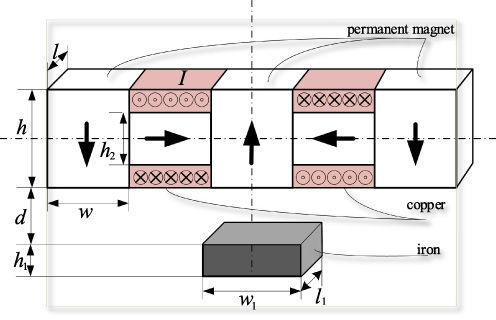
Hybrid magnet based on Halbach array.

5.1. Introduction to GRNN

The GRNN was proposed by Donald F. Spect. The GRNN network has a strong nonlinear fitting ability and provides good prediction results even when there is a small amount of sample data, which is suitable for the situation in which the electromagnetic actuator designed in this study cannot obtain a large amount of collected data. The GRNN has four layers, as shown in Fig. 5; namely, Input Layer, Pattern Layer, Summation Layer and Output Layer from input to output. The network input is X = [x ₁, x ₂…, x _n]^T and the output is Y = [y ₁, y ₂, …, y _k]^T.

Fig. 5.

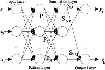
Generalized regression neural network structure.

Parzen non-parametric estimation is adopted in the GRNN, and the final network output value is expressed as $\begin{eqnarray}\displaystyle {\hat{Y}}(X)=\frac{\displaystyle \mathop{\sum }_{i=1}^{n}Y_{i}\exp \left[-\frac{(X-X_{i})^{T}(X-X_{i})}{2{\sigma}^{2}}\right]}{\displaystyle \mathop{\sum }_{i=1}^{n}\exp \left[-\frac{(X-X_{i})^{T}(X-X_{i})}{2{\sigma}^{2}}\right]} & & \displaystyle\end{eqnarray}$ (26) where, ${\hat{Y}}(X)$ is the weighted average value Y _i of all sample observations. X _i is the learning sample corresponding to the ith neuron, while σ is the width coefficient of the Gaussian function when Parzen non-parametric estimation is applied. Also, σ is called the smoothing factor. When the value of the smoothing factor is large, the estimated value is close to the sample mean, and when the smoothing factor is small, the generalization ability of the network is poor. In other words, the theoretical essence of the GRNN neural network is nonlinear regression analysis, and the equation solves the y value with maximum probability. And ${\hat{Y}}(X)$ is denoted as the predicted output of Y under the condition that the input is X. It can be concluded from the equation and related studies [49] that the value of the smoothing factor determines the prediction accuracy of the network; thus, the value of the smoothing factor needs to be weighed. we can use the modified AO algorithm for finding the optimal value.

5.2. Basic principle of the experiment

5.2.1. Data collection

The improved GRNN flow chart is shown in Fig. 6. Before the data are predicted, the normalized sample data are divided into a training group and testing group, and the smoothing factor is initialized as the input of the algorithm. The GRNN makes its prediction using the training group data in the dataset and the input smoothing factor, takes the mean square error of normalized prediction results as the fitness value of the corresponding solution (smoothing factor), and iterates within the algorithm until it finally outputs the prediction result and the corresponding mean squared error. This paper mainly discusses the effectiveness and feasibility of the field research method. Moreover, actual experiments require a lot of time and cost due to the problem of manufacturing permanent magnets of different sizes and shapes. The effectiveness of the algorithm is verified using Ansoft simulation experimental data. The same number of data available for real design are simulated, and 30 groups of experiments are set up. The dataset includes 30 groups of overall data. Twenty-two groups of data are selected as training data, another five groups of data are used as validation data, and the remaining three groups of data are used as testing data. The training data and validation data form the training group data. The training group data are used for training and optimization, and the testing group data is used to test the results. The output variable is the magnetic force F of suspended objects, and the input variable includes the length l, width w, and height (h) of Halbach array, the current intensity (I), the coil related size (h ₂), the distance between suspended objects and the array surface (d), and the length (l ₁), width w ₁, and height (h ₁) of suspended objects. Additionally, to prevent there being accidental errors in the simulation, we conduct the simulation 10 times for each group of data and take the average value of the results as the result for that group. The following measures are taken to prevent the overfitting of the prediction.

The data are normalized before training.

After the algorithm optimization, the training data and validation data are randomly adjusted in the training group data, and optimization is performed again until the validation count is reached.

Fig. 6.

Flow chart of the improved GRNN.

5.2.2. Regression model

In the GRNN optimized by the algorithm, the iteration number of the algorithm is set as 1000, the population is set as 30, the number of validation is set to 10, and the smoothing factor (σ) range is set as [0, 2]. The algorithm was run ten times with consistent parameter settings during each run. The other factors in the algorithm remained unchanged after each run. The average of the run results was used as the final optimization result. After optimization, the optimal smoothing factor was 1.3037. The iterative process is illustrated in Fig. 7. However, it can be observed that the algorithm converges to the optimal value in the first 100 generations. The MSE value of the normalized prediction results corresponding to the smoothing factor was 0.1404.

Fig. 7.

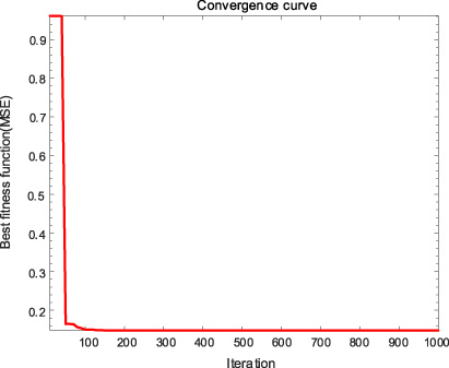
The iterative process.

5.3. Comparison of simulation experiment results

To further verify the prediction effect of the improved GRNN, the radial basis function (RBF) and KCV (K-fold Cross Verified)-GRNN network were compared. The radial basis function expansion speed is set to 30. Three datasets (A, B, C) were randomly selected from Table 4 with different amounts of data. The testing data in each dataset were the same. The amounts of each type of data in each dataset are shown in the Table 5. The prediction results of the three prediction models in dataset A, B, C and their relative errors are shown in Fig. 8. Table 6 shows the goodness of fit(R ²) and normalized mean square error of the prediction model.

Table 4
The dataset

d/mm I/A w/mm h ₂ /mm h/mm l/mm l ₁ /mm w ₁ /mm h ₁ /mm F/N

1 10 3 30 40 60 30 30 20 5 23.024

2 20 3.5 35 35 55 35 40 25 10 17.541

3 10 4 40 30 50 40 30 20 15 65.121

4 20 4.5 45 25 45 45 40 10 10 15.459

5 10 5 50 20 40 50 20 30 10 43.321

6 20 5.5 55 15 35 55 30 20 10 16.165

7 10 6 60 10 30 60 40 20 5 17.883

8 20 5.5 55 10 35 55 30 25 15 22.555

9 10 2.5 50 30 40 50 20 20 10 39.568

10 20 2.25 45 35 45 45 30 30 5 17.357

11 10 6 40 20 50 40 40 30 15 79.866

12 20 5.25 35 25 55 35 20 10 10 7.388

13 10 6 30 40 60 30 40 15 10 40.039

14 20 1 50 20 40 50 30 20 5 5.816

15 10 2 55 15 35 55 40 25 10 37.059

16 20 1.5 60 10 30 60 30 20 15 13.317

17 10 1 55 10 35 55 40 10 10 24.222

18 20 1.25 50 30 40 50 20 30 10 5.732

19 10 0.75 45 35 45 45 30 20 10 19.342

20 20 1.2 40 20 50 40 40 20 5 19.228

21 10 1.5 35 25 55 35 30 25 15 44.029

22 20 1.35 30 40 60 30 20 20 10 3.287

23 10 0.95 40 30 50 40 30 30 5 21.929

24 20 2.25 45 25 45 45 40 30 15 15.995

25 10 2.05 50 20 40 50 20 10 10 13.149

26 20 1.15 55 15 35 55 40 15 10 9.976

27 10 0.5 30 40 60 30 30 30 5 3.577

28 20 1.8 35 35 55 35 20 30 10 5.470

29 10 1.7 40 30 50 40 30 10 15 24.243

30 20 1.6 45 25 45 45 40 15 10 8.609

	d/mm	I/A	w/mm	h ₂ /mm	h/mm	l/mm	l ₁ /mm	w ₁ /mm	h ₁ /mm	F/N
1	10	3	30	40	60	30	30	20	5	23.024
2	20	3.5	35	35	55	35	40	25	10	17.541
3	10	4	40	30	50	40	30	20	15	65.121
4	20	4.5	45	25	45	45	40	10	10	15.459
5	10	5	50	20	40	50	20	30	10	43.321
6	20	5.5	55	15	35	55	30	20	10	16.165
7	10	6	60	10	30	60	40	20	5	17.883
8	20	5.5	55	10	35	55	30	25	15	22.555
9	10	2.5	50	30	40	50	20	20	10	39.568
10	20	2.25	45	35	45	45	30	30	5	17.357
11	10	6	40	20	50	40	40	30	15	79.866
12	20	5.25	35	25	55	35	20	10	10	7.388
13	10	6	30	40	60	30	40	15	10	40.039
14	20	1	50	20	40	50	30	20	5	5.816
15	10	2	55	15	35	55	40	25	10	37.059
16	20	1.5	60	10	30	60	30	20	15	13.317
17	10	1	55	10	35	55	40	10	10	24.222
18	20	1.25	50	30	40	50	20	30	10	5.732
19	10	0.75	45	35	45	45	30	20	10	19.342
20	20	1.2	40	20	50	40	40	20	5	19.228
21	10	1.5	35	25	55	35	30	25	15	44.029
22	20	1.35	30	40	60	30	20	20	10	3.287
23	10	0.95	40	30	50	40	30	30	5	21.929
24	20	2.25	45	25	45	45	40	30	15	15.995
25	10	2.05	50	20	40	50	20	10	10	13.149
26	20	1.15	55	15	35	55	40	15	10	9.976
27	10	0.5	30	40	60	30	30	30	5	3.577
28	20	1.8	35	35	55	35	20	30	10	5.470
29	10	1.7	40	30	50	40	30	10	15	24.243
30	20	1.6	45	25	45	45	40	15	10	8.609

Table 5

Amounts of each type of data

	Training data	Validation data	Testing data	Dataset
A	14	3	3	20
B	18	4	3	25
C	22	5	3	30

Fig. 8.

Comparison of prediction.

Table 6

Goodness of fit and mean square error of normalized prediction results

		Improved-GRNN	KCV-GRNN	RBF
A	MSE	0.1454	0.2485	0.3633
	R ²	0.8347	0.7361	0.6588
B	MSE	0.1485	0.2554	0.2420
	R ²	0.8388	0.7478	0.4671
C	MSE	0.1404	0.2453	0.4455
	R ²	0.8414	0.7441	0.4847

Figure 8 shows that the prediction results of the GRNN prediction model based on the improved algorithm are close to the real values for different datasets. It can be observed that the prediction results of improved GRNN for the testing data differed less in different numbers of datasets. The relative error of the prediction results of the modified GRNN is almost less than 10%, which outperforms KCV-GRNN and RBF. And the relative error of the prediction results of the KCV-GRNN model is around 35%. Looking at Table 6, it can be seen that: (1) the MSE and R ² values of the improved GRNN model are relatively stable even in datasets with different amounts of data; (2) the R ² values of each dataset of GRNN prediction models based on the improved algorithm is higher than that of KCV-GRNN and RBF, and the mean square error is lower than that of KCV-GRNN and RBF. Therefore, we know that GRNN has better prediction performance on a certain amount of data, and the limitation of the amount of data has less impact on improved GRNN. Collectively, the prediction performance of GRNN prediction models based on the improved algorithm exceeds that of other two prediction models.

The results show that the modified AO algorithm has improved accuracy of the GRNN and provides ideas for the improvement of the prediction model. In terms of efficiently designing an electromagnetic actuator, at present, the finite element method is mainly used to simulate and analyze the structure. However, considering the restrictions that we described earlier, there will be large errors in the theoretical design and simulation results. Therefore, in practical application, we usually design an electromagnetic actuator based on an empirical structure or simulation experiment size and build a test device to verify the results. However, it is considered that the complexity of variable combinations introduces difficulties in structural design. We therefore build a small number of experimental groups in the preliminary stage of the electromagnetic structural design, obtain the required experimental results, roughly determine the demand range, and train the GRNN to predict the experimental results for specific structural parameters using data and the improved algorithm, so as to provide effective guidance for the design of the electromagnetic actuator. Although the neural-network prediction method has limitations in data application, with the progress of science and technology and intelligent systems, the performance of the method can be continuously improved by expanding the calculation parameters and research fields.

6. Conclusion

This paper proposed a modified adaptive AO, whereby a normal distribution is adopted for the random parameter generation, and an adaptive speed factor and Weibull adaptive distribution function are included the Aquila capturing process. Benchmark function tests showed that the (Modified AO) algorithm has higher accuracy and efficiency than the WHO, ACO, and PSO algorithms and the original AO algorithm, and the improved method has certain effectiveness and thus provides a reference for improvements to other heuristic algorithms.

In this paper, the modified AO algorithm was used to improve the GRNN. The algorithm was applied to the prediction of the electromagnetic force of an electromagnetic actuator. The algorithm was trained using 30 groups of simulation data, including twenty-seven groups of data for training and three groups of data for testing. The mean squared error of the improved GRNN prediction result reached 0.1404. The improved GRNN model was thus shown to be feasible and to have certain reference importance for the design of an electromagnetic actuator.

The paper compared the improved GRNN with RBF and KCV-GRNN algorithm. The results show that the GRNN had advantages in prediction for small-sample data, and the use of the improved algorithm afforded the neural network better prediction performance. The relative error of the prediction results of the improved GRNN prediction model was almost less than 10%, with higher accuracy. The proposed method provides guidance and a research direction for the application of the AO algorithm in prediction.

Footnotes

Acknowledgements

This work is fully supported by the Nation Natural Science Foundation of China (51874004, 51904007), Key Research and Development Project of Anhui Province (202004a07020043), the Nature Science Foundation of Anhui Province (1908085QE227), National Key Research and Development Program Sub-Task(2020YFB1314203).

We thank Liwen Bianji (Edanz) (www.liwenbianji.cn) and Editage () for editing the language of a draft of this manuscript.

References

Choudhury

H.A.

Sinha

and Saikia

, Nature inspired algorithms (NIA) for efficient video compression – A brief study, Engineering Science and Technology-an International Journal-Jestech 23(3) (2020), 507–526.

Abualigah

, Group search optimizer: A nature-inspired meta-heuristic optimization algorithm with its results, variants, and applications, Neural Computing & Applications 33(7) (2021), 2949–2972.

Eberhart

and Kennedy

, A new optimizer using particle swarm theory, in: MHS’95. Proceedings of the Sixth International Symposium on Micro Machine and Human Science, 1995, pp. 39–43. doi:10.1109/MHS.1995.494215.

Karaboga

and Basturk

, A powerful and efficient algorithm for numerical function optimization: Artificial bee colony (ABC) algorithm, Journal of Global Optimization 39(3) (2007), 459–471.

Dorigo

Maniezzo

and Colorni

, Ant system: Optimization by a colony of cooperating agents, IEEE Transactions on Systems, Man, and Cybernetics. Part B, Cybernetics: A Publication of the IEEE Systems, Man, and Cybernetics Society 26(1) (1996), 29–41.

Das

A.K.

and Pratihar

D.K.

, Bonobo optimizer (BO): An intelligent heuristic with self-adjusting parameters over continuous spaces and its applications to engineering problems, Applied Intelligence 52 (2021), 2942–2974.

Abualigah

Yousri

Abd Elaziz

Ewees

A.A.

Al-qaness

M.A.A.

and Gandomi

A.H.

, Aquila optimizer: A novel meta-heuristic optimization algorithm, Computers & Industrial Engineering 157 (2021), doi:10.1016/j.cie.2021.107250.

Holland

J.H.

, Genetic algorithms, Scientific American 267(1) (1992), 66–73.

Storn

and Price

, Differential evolution–a simple and efficient heuristic for global optimization over continuous spaces, Journal of Global Optimization 11(4) (1997), 341–359.

10.

Tang

Dong

Jiang

and Huang

, ITGO: Invasive tumor growth optimization algorithm, Applied Soft Computing 36 (2015), 670–698.

11.

Rashedi

Nezamabadi-Pour

and Saryazdi

, GSA: A gravitational search algorithm, Information Sciences 179(13) (2009), 2232–2248.

12.

Formato

R.A.

, Central force optimization: A new metaheuristic with applications in applied electromagnetics, Progress in Electromagnetics Research-Pier 77 (2007), 425–491.

13.

Rao

R.V.

Savsani

V.J.

and Vakharia

D.P.

, Teaching-learning-based optimization: An optimization method for continuous non-linear large scale problems, Information Sciences 183(1) (2012), 1–15.

14.

Watkins

C.J.

and Dayan

, Q-learning, Machine Learning 8(3) (1992), 279–292.

15.

Sutton

R.S.

and Barto

A.G.

, Reinforcement learning: An introduction, IEEE Transactions on Neural Networks 9(5) (1998), 1054.

16.

Elsisi

, Future search algorithm for optimization, Evolutionary Intelligence 12(1) (2018), 21–31.

17.

Mnih

Kavukcuoglu

Silver

Rusu

A.A.

Veness

Bellemare

M.G.

, Human-level control through deep reinforcement learning, Nature 518(7540) (2015), 529–533.

18.

Gong

and Zhu

, Four-factor polarity switching control for synchronous vibration suppression of active magnetic bearings rigid rotors system in the full rotational speed range, IEEE Transactions on Industrial Electronics 68(12) (2021), 11870–11880.

19.

Molina

L.M.C.

Bonfitto

and Galluzzi

, Offset-free model predictive control for a cone-shaped active magnetic bearing system, Mechatronics 78 (2021), doi:10.1016/j.mechatronics.2021.102612.

20.

and Zhou

, Comparisons on the six-pole hybrid magnetic bearing under two control methods, IEEE Transactions on Applied Superconductivity 31(8) (2021), 1–4.

21.

Yang

Jiang

Sun

and Liu

, Series-winding topology converter for active magnetic bearing drive, IEEE Transactions on Industrial Electronics 68(12) (2021), 11772–11782.

22.

Zhang

and Zhu

, Dynamic correction model considering influence of foundation motions for a centripetal force type-magnetic bearing, IEEE Transactions on Industrial Electronics 68(10) (2021), 9811–9821.

23.

Zhang

Zhu

Wang

and Zhu

, Stability control for a centripetal force type-magnetic bearing-rotor system based on golden frequency section point, IEEE Transactions on Industrial Electronics 68(12) (2021), 12482–12492.

24.

Han

J.-B.

and Kim

K.-J.

, Characteristics of vibration in magnetically levitated trains subjected to crosswind, Proceedings of the Institution of Mechanical Engineers Part F-Journal of Rail and Rapid Transit 232(5) (2018), 1347–1359.

25.

Hasirci

Balikci

Zabar

and Birenbaum

, A novel magnetic-levitation system: Design, implementation, and nonlinear control, IEEE Transactions on Plasma Science 39(1) (2011), 492–497.

26.

de Oliveira

R.A.H.

Stephan

R.M.

and Ferreira

A.C.

, Optimized linear motor for urban superconducting magnetic levitation vehicles, IEEE Transactions on Applied Superconductivity 30(5) (2020), 1–8.

27.

Delikoyun

Yaman

Yilmaz

Sarigil

Anil-Inevi

Telli

, HologLev: A hybrid magnetic levitation platform integrated with lensless holographic microscopy for density-based cell analysis, Acs Sensors 6(6) (2021), 2191–2201.

28.

Durmus

Gupta

Badamjav

Reddy

Eisenberg

M.L.

Behr

, A magnetic levitation platform for the isolation of mature sperm from TESE/TESA samples, Fertility and Sterility 109(3) (2018), 26–27.

29.

Lin

Oka

and Harada

, Zero-power tip-tilt control of a magnetically levitated platform by lateral displacement of hybrid-electromagnets, International Journal of Applied Electromagnetics and Mechanics 66(1) (2021), 63–74.

30.

Mehrtash

and Khamesee

M.B.

, Modeling and analysis of eddy-current damping effect in horizontal motions for a high-precision magnetic navigation platform, IEEE Transactions on Magnetics 49(8) (2013), 4801–4810.

31.

Silva

B.E.

and Barbosa

R.S.

, Experiments with neural networks in the identification and control of a magnetic levitation system using a low-cost platform, Applied Sciences-Basel 11(6) (2021), doi:10.3390/app11062535.

32.

Verderber

McKnight

and Bozkurt

, Electromagnetic levitation platform for wireless study of insect flight neurophysiology, in: Annual International Conference of the IEEE Engineering in Medicine and Biology Society. IEEE Engineering in Medicine and Biology Society. Annual International Conference, Vol. 2013, 2013, pp. 1720–1723.

33.

Shi

and Wang

, 3D analytical model of drag and lift force for a conductive plate moving above a Halbach magnet array, Transactions of the Institute of Measurement and Control 40(12) (2018), 3515–3524.

34.

Golovanov

and Gerada

, An analytical subdomain model for dual-rotor permanent magnet motor with Halbach array, IEEE Transactions on Magnetics 55(12) (2019), 1–16.

35.

Lee

Jung

and Yoo

, Topology optimization for three-dimensional design of segmented permanent magnet arrays, Structural and Multidisciplinary Optimization 62(6) (2020), 3089–3104.

36.

Zhou

Wang

and He

, Torque calculation of permanent-magnet spherical motor based on permanent-magnet surface current and lorentz force, IEEE Transactions on Magnetics 56(5) (2020), 1–9.

37.

Cansiz

Reisoglu

A.F.

Ozturk

and Abdioglu

, Frozen image analysis of a superconducting magnetic levitation system consisting of multi-surface superconductor and Halbach array permanent magnet configuration, Cryogenics 117 (2021), doi:10.1016/j.cryogenics.2021.103328.

38.

Wang

and Zhou

, Unbalanced magnetic torque in electrohydraulic energy conversion unit considering rotor axis deflection, IEEE Transactions on Magnetics 52(6) (2016), 1–6.

39.

Kou

Xing

Zhang

and Zhou

, A real-time computation model of the electromagnetic force and torque for a maglev planar motor with the concentric winding, Applied Sciences-Basel 7(1) (2017), doi:10.3390/app7010098.

40.

Asef

Perpina

R.B.

Barzegaran

M.R.

Lapthorn

and Mewes

, Load identification of different Halbach-array topologies on permanent magnet synchronous generators using the coupled field-circuit FE methodology, Electric Power Systems Research 154 (2018), 484–492.

41.

Cooley

C.Z.

Haskell

M.W.

Cauley

S.F.

Sappo

Lapierre

C.D.

C.G.

, Design of sparse Halbach magnet arrays for portable MRI using a genetic algorithm, IEEE Transactions on Magnetics 54(1) (2018), 1–12.

42.

Cui

and Li

, Multi-objective optimization of the Halbach array permanent magnet spherical motor based on support vector machine, Energies 13(21) (2020), doi:10.3390/en13215704.

43.

Zheng

Zhang

and Hong

, Track defect detection for high-speed maglev trains via deep learning, IEEE Transactions on Instrumentation and Measurement 71 (2022), 1–8.

44.

Deng

Chen

Liu

Wang

, Vibration states detection of HTS pinning maglev system based on deep learning algorithm, IEEE Transactions on Applied Superconductivity 32(6) (2022), 1–6.

45.

Liu

Chen

Shi

and Deng

, Prediction models establishment and comparison for guiding force of high-temperature superconducting maglev based on deep learning algorithms, Superconductor Science & Technology 35(2) (2022), 1–8.

46.

Liu

Chen

and Deng

, The feasibility of designing a back propagation neural network to predict the levitation force of high-temperature superconducting magnetic levitation, Superconductor Science & Technology 35(4) (2022), 1–5.

47.

Sun

Lin

and Mumtaz

, Deep learning based semi-supervised control for vertical security of maglev vehicle with guaranteed bounded airgap, IEEE Transactions on Intelligent Transportation Systems 22(7) (2021), 4431–4442.

48.

Zhao

You

Song

Zhang

and Tong

, Suspension regulation of medium-low-speed maglev trains via deep reinforcement learning, IEEE Transactions on Artificial Intelligence 2(4) (2021), 341–351.

49.

Qiao

Liu

Zhu

and Wang

, Machine-learning approach to predict work hardening behavior of pearlitic steel, Materials Letters 289 (2021), doi:10.1016/j.matlet.2021.129384.

50.

Qiao

Wang

and Zhu

, Application of improved GRNN model to predict interlamellar spacing and mechanical properties of hypereutectoid steel, Materials Science and Engineering a-Structural Materials Properties Microstructure and Processing 792 (2020), doi:10.1016/j.msea.2020.139845.

51.

Sanikhani

Kisi

Maroufpoor

and Yaseen

Z.M.

, Temperature-based modeling of reference evapotranspiration using several artificial intelligence models: Application of different modeling scenarios, Theoretical and Applied Climatology 135(1–2) (2019), 449–462.

52.

Jafari

and Shahsavar

, The application of artificial neural networks in modeling and predicting the effects of melatonin on morphological responses of citrus to drought stress, PLoS One 15(10) (2020), doi:10.1371/journal.pone.0240427.

53.

Sridharan

, Application of generalized regression neural network in predicting the performance of natural convection solar dryer, Journal of Solar Energy Engineering-Transactions of the ASME 142(3) (2020), doi:10.1115/1.4045384.

54.

Liu

and Sun

, Application of the fruit fly optimization algorithm to an optimized neural network model in radar target recognition, Computer Optics 45(2) (2021), 296–300.

55.

Sridharan

and Shenbagaraj

, Application of generalized regression neural network in predicting the thermal performance of solar flat plate collector systems, Journal of Thermal Science and Engineering Applications 13(2) (2021), doi:10.1115/1.4047824.

56.

Alrassas

A.M.

Al-qaness

M.A.A.

Ewees

A.A.

Ren

Abd Elaziz

Damasevicius

, Optimized ANFIS model using aquila optimizer for oil production forecasting, Processes 9(7) (2021), doi:10.3390/pr9071194.

57.

Chung

, The golden ratio’s essential attributes and utilization measures, A Treatise on The Plastic Media 18(1) (2015), 139–148.

58.

Hoefer

and Buss

, Assessing and improving model fitness in MOCABA data assimilation, Annals of Nuclear Energy 162 (2021), doi:10.1016/j.anucene.2021.108490.

59.

Hretcanu

C.-E.

and Crasmareanu

M.-C.

, Applications of the golden ratio on Riemannian manifolds, Turkish Journal of Mathematics 33(2) (2009), 179–191.

60.

Lee

M.H.

, Application of golden ratio jacket code in MIMO wireless communications, The Journal of The Institute of Internet, Broadcasting and Communication 17(4) (2017), 83–93.

61.

Ryu

Kanemaru

Kataoka

Arihama

Yoshitake

Arakawa

, Optimization of energy saving device combined with a propeller using real-coded genetic algorithm, International Journal of Naval Architecture and Ocean Engineering 6(2) (2014), 406–417.

62.

Xie

Weerasekara

N.N.

and Issa

R.R.A.

, Improved system for modeling and simulating stadium evacuation plans, Journal of Computing in Civil Engineering 31(3) (2017), doi:10.1061/(ASCE)CP.1943-5487.0000634.

63.

Yun

, A study on golden ratio as a universal principle of modern design, Journal of the Korean Society of Design Culture 15(3) (2009), 279–288.

64.

Zhang

, An improved high-moment method for reliability analysis, Structural and Multidisciplinary Optimization 56(6) (2017), 1225–1232.

65.

Azimi

and Esmailian

, Correction to: The Weibull Frechet distribution and its applications, Journal of Applied Statistics 48(16) (2021), 3251–3252.

66.

Cordeiro

G.M.

Saboor

Khan

M.N.

Ozel

and Pascoa

M.A.R.

, The Kumaraswamy exponential-Weibull distribution: Theory and applications, Hacettepe Journal of Mathematics and Statistics 45(4) (2016), 1203–1229.

67.

Dokur

Ceyhan

and Kurban

, Finsler geometry for two-parameter Weibull distribution function, Mathematical Problems in Engineering (2017), doi:10.1155/2017/9720946.

68.

Liao

Ahmad

Mahmoudi

and Hamedani

G.G.

, A new flexible bathtub-shaped modification of the Weibull model: Properties and applications, Mathematical Problems in Engineering (2020), doi:10.1155/2020/3206257.

69.

Shamshirband

Mohammadi

Tong

C.W.

Petkovic

Porcu

Mostafaeipour

, Application of extreme learning machine for estimation of wind speed distribution, Climate Dynamics 46(5–6) (2016), 1893–1907.

70.

Singla

Jain

and Sharma

S.K.

, The Beta Generalized Weibull distribution: Properties and applications, Reliability Engineering & System Safety 102 (2012), 5–15.

71.

Tahir

M.H.

Cordeiro

G.M.

Mansoor

Zubair

and Alizadeh

, The Weibull–Dagum distribution: Properties and applications, Communications in Statistics-Theory and Methods 45(24) (2016), 7376–7398.

72.

Yunhwan

and Shik

C.Y.

, Inverted exponentiated Weibull distribution with applications to lifetime data, Communications for Statistical Applications and Methods 24(3) (2017), 227–240.

73.

Naruei

and Keynia

, Wild horse optimizer: a new meta-heuristic algorithm for solving engineering optimization problems, Engineering with Computers (2021), doi:10.1007/s00366-021-01438-z.

74.

Dorigo

and Maniezzo

, Ant system: optimization by a colony of cooperating agents, IEEE Trans. on SMC-Part B 26(1) (1996), 29.

Magnetic force prediction of hybrid magnet with Halbach array using generalized regression neural network optimized by a modified aquila optimizer

Abstract

1. Introduction

2. AO algorithm

3.1. Random-parameter modification

Table 1 Algorithms used for comparative analysis and their population settings. NFEs denotes the number of objective function evaluations Algorithm Population size NFEs AO 30 30000 Modified AO 30 30000 WHO 30 30000 ACO 30 30000 PSO 30 30000

5.2.1. Data collection

Footnotes

Acknowledgements

References

Table 1
Algorithms used for comparative analysis and their population settings. NFEs denotes the number of objective function evaluations

Algorithm Population size NFEs

AO 30 30000

Modified AO 30 30000

WHO 30 30000

ACO 30 30000

PSO 30 30000