
Abstract
A water pipe used underwater is required as a method of supplying domestic water to remote islands. In order to ensure this safety, it is necessary to develop maintenance technology for underwater structures. In this research, the deterioration state of the water pipe is clarified, and the remaining life is judged by electromagnetic non-destructive inspection. This method uses the pulse ECT technology.
Introduction
The undersea water pipe technology is responsible for supplying daily life water to remote islands, and it is necessary to ensure safety. Recently, the problem is that the aged deterioration of water pipes is faster than expected. These may cause accidents such as water leakage, breakage, and water pollution of the water pipe. These are due to defects and wall thinning caused by seawater and earthquakes. In order to prevent accidents, it is necessary to know the location of leaks and the size of defects. However, since the deterioration state inside the water pipe cannot be grasped, the life of the water pipe cannot be judged. In this research, an inspection method that can visualize the deterioration inside the water pipe using electromagnetic non-destructive inspection technology is proposed. The proposed electromagnetic sensor is applied from outside the water pipe. It is possible to inspect not only defects on the surface of pipes but also defects on the inner surface. In addition, inspection can be performed without stopping the operation of piping. The proposed electromagnetic sensor applies a pulse eddy current testing (pulse ECT) that is not easily affected by the measurement distance [1,2]. The proposed method evaluates the decay time of the detected voltage signal obtained by generating four magnetically closed loops. The proposed inspection method is investigated by the 3-D nonlinear FEM taking account of hysteresis magnetizing properties and eddy current in the steel tube [3,4].
The proposed electromagnetic sensor model.
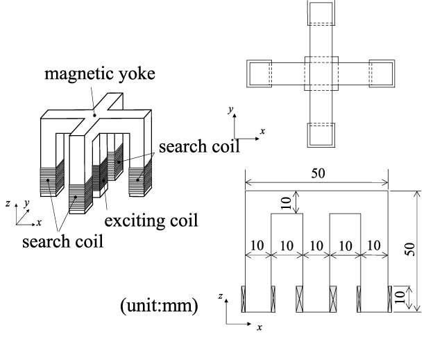
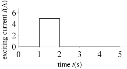
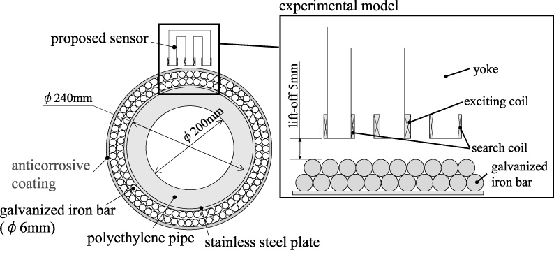
Figure 1 shows the proposed electromagnetic sensor model. The magnetic yoke is in the shape of a cross with five legs. The proposed electromagnetic sensor is composed of an exciting coil (40 turns) and four search coils (200 turns). A magnetic field is applied from the foot in the center of the yoke material. The search coil uses four legs of the yoke material around the exciting coil. As for the search coil in this sensor, the z-direction flux density (B z ) is detected. These four search coils are connected in parallel and detect the induced electromotive force generated in each coil. Figure 2 shows the pulse exciting current waveform. The amplitude of pulse exciting current is a rectangle wave of 5 A for 1 second. Figure 3 shows the measurement model of a water pipe and an electromagnetic sensor. The water pipe to be inspected has an inner diameter of 200 mm, and the total diameter is about 300 mm. In this research, the inspection target is a water pipe whose polyethylene pipe is covered with a galvanized iron bar (𝜙 6 mm). The layer of the galvanized iron bar is composed of two layers. The anticorrosive coating does not consist of a conductive material. In the experiment, the defective state of this iron bar part is inspected. The experimental model consists of stainless steel plate and galvanized iron bar layer. There is a distance of 5 mm between the proposed electromagnetic sensor and the galvanized iron bar layer.
Experimental result and defect estimation method
Proposal of output voltage signal processing method
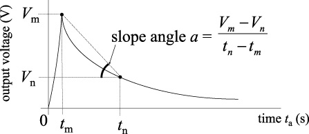
In the proposed method, the output voltage signal obtained in the search coil is evaluated by the slope angle a. Figure 4 shows the outline of the output voltage waveform in the search coil after cutting off the pulsed wave magnetic field. This slope angle is calculated by the following formula.
The pulse exciting current waveform.
The measurement model of a water pipe and an electromagnetic sensor.
Outline of the output waveform in the search coil.
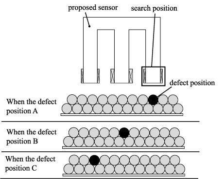
The model when a defect occurs on the surface of the iron bar layer.
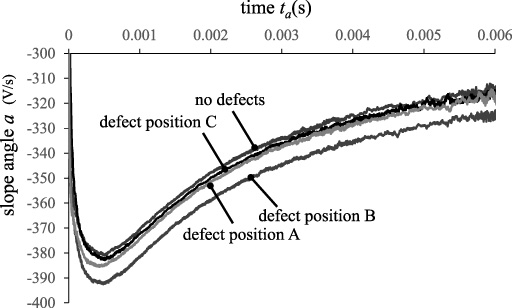
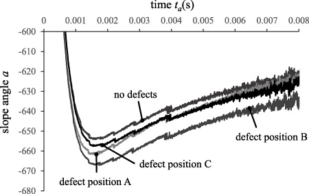
The experimental results when a defect occurs on the surface of the iron bar layer.
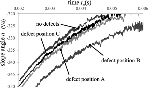
The enlarged waveform between 0.002 s to 0.006 s of the experimental results shown in Fig. 6.
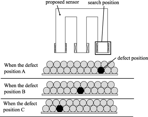
The model when a defect occurs on the inside of the iron bar layer.
The experimental results when a defect occurs on the inside of the iron bar layer.
The experimental results show the output voltage signal for one search coil. Figure 5 shows the model when a defect occurs on the surface of the iron bar layer. There are three types of defects used in the experiment. Defect position A is the case where a defect occurs in the position of the search coil that measures the output voltage signal. Defect position B is the case where a defect occurs in the position of the exciting coil. Defect position C is the case where a defect occurs at the position of the search coil that is the longest distance from the search coil that measures the output voltage signal. Figure 6 shows the experimental results when a defect occurs on the surface of the iron bar layer. Figure 7 shows the enlarged waveform between 0.002 s to 0.006 s of the experimental results shown in Fig. 6. The horizontal axis and the vertical axis in this figure are the time (t a ) after cutting off the pulsed exiting magnetic field, and the slope angle a from the maximum value of the output voltage in the search coil, respectively. From the results in the figure, it can be seen that the slope angle a obtained from the output voltage signal shown in Fig. 4 decreases due to the occurrence of the defect. the slope angle a is most reduced when there is a defect in the position of the exciting coil. There is a difference in the slope angle a of the defect position A and the defect position C between 0.000 s to 0.001 s immediately after the pulse magnetic field is cut off. However, a similar slope angle a can be obtained in the time after 0.003 s. Figure 8 shows the model when a defect occurs on the inside of the iron bar layer. There are three types of defects used in the experiment. Defect position A is the case where a defect occurs in the position of the search coil that measures the output voltage signal. Defect position B is the case where a defect occurs in the position of the exciting coil. Defect position C is the case where a defect occurs at the position of the search coil that is the longest distance from the search coil that measures the output voltage signal. Figure 9 shows the experimental results when a defect occurs on the inside of the iron bar layer. The horizontal axis and the vertical axis in this figure are the time (t a ) after cutting off the pulsed exiting magnetic field, and the slope angle a from the maximum value of the output voltage in the search coil. This figure denotes that when the position of the defect is the exciting coil (defect position B), the slope angle a from the case where there is no defect is the maximum. Also, the slope angle a has a difference between the defect position A and the defect position C in 0.01 to 0.02 seconds after the pulse magnetic field is cut off, but the output signal becomes the same in 0.04 to 0.06 seconds.
Inspection of water pipe defect by 3D non-linear FEM
In this analysis, a pulse magnetic field is applied to the iron bar layer, the flux density and eddy current inside the iron bar layer is calculated using the 3-D nonlinear FEM taking account of hysteresis curves as shown in Fig. 10.
The basic equation of eddy current analysis using the
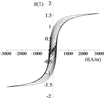
Hysteresis curves of the steel plate and steel metal.
Conditions of calculation and experiment
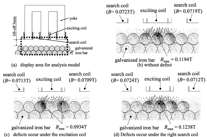
Magnetic flux distribution during application of pulsed magnetic field.
The analysis was performed und er the same conditions as in the experiment, with 40 turns for the exciting coil and 200 turns for the search coil. The conductivity of the galvanized iron bar is 7.5 × 10⁶ S/m. The convergence judgment values of N-R method and ICCG method are 1.0 × 10⁻⁴ T and 1.0 × 10⁻⁴, respectively. The time interval of the step-by-step method is chosen as 1.0 × 10⁻³ second. The distance between (lift-off) the proposed electromagnetic sensor and the galvanized iron bar layer is 5 mm.
Figure 11 shows the magnetic flux distribution while the pulse magnetic field is applied. Figure 11(a) shows the display area. Figure 11(b) shows the magnetic flux distribution when no defect has occurred. Figure 11(c) shows the magnetic flux distribution when a defect occurs under the exciting coil. Figure 11(d) shows the magnetic flux distribution when a defect occurs under the search coil on the right side of the model. From this figure, it can be seen that the maximum magnetic flux density is obtained under the exciting coil while the pulse magnetic field is applied. The magnitude of the maximum magnetic flux density changes at the position of the defect. When there is a defect under the exciting coil, the maximum magnetic flux density is decreased than when there is no defect. When there is a defect under the search coil, the maximum magnetic flux density is increased than when there is no defect. In addition, when a defect occurs under the search coil, the difference between the magnetic flux density values of the left and right search coils becomes the largest. The maximum difference of 0.0012 T is shown in Fig. 11(d). This is because the left and right magnetic experimental fluxes model are not balanced due to the defect.
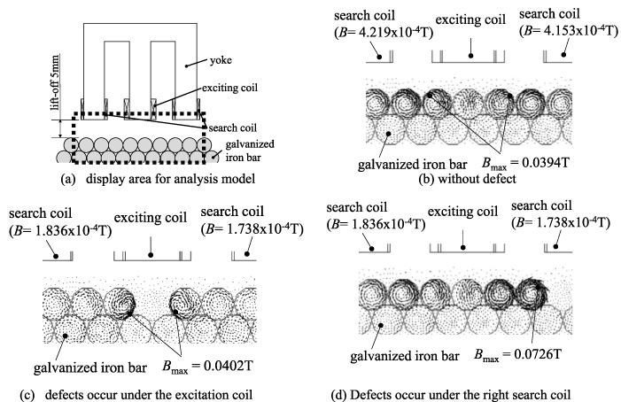
Magnetic flux distribution after pulsed magnetic field cutoff (t a = 0.003 s).
Figure 12 shows the magnetic flux distribution 0.003 seconds after the pulse magnetic field is cut off. Figure 12(a) shows the display area. Figure 12(b) shows the magnetic flux distribution when no defect has occurred. Figure 12(c) shows the magnetic flux distribution when a defect occurs under the exciting coil. Figure 12(d) shows the magnetic flux distribution when a defect occurs under the search coil on the right side of the model. From this result, it can be seen that the magnetic flux is rotating in the iron rod after the pulse magnetic field is cut off. In addition, it can be seen that a large magnetic flux is generated on the surface layer in the region between the exciting coil and the search coil. When a defect occurs, it can be seen that the maximum magnetic flux density is obtained with the iron rod next to the defect. From this, it can be seen that the magnetic fluxes are canceled by the adjacent iron bars after the pulse magnetic field is cut off. When a defect occurs, cancellation does not occur. Therefore, it was found that the magnetic flux near the defect became large. The magnetic flux densities obtained from the left and right search coils also have the same difference as that in Fig. 11 without defects. The maximum difference of 9.8 × 10⁻⁶ T is shown in Fig. 11(c) and Fig. 11(d). It can be seen that the magnetic flux density obtained from the search coil is the lowest when the exciting coil is defective. This is because the magnetic flux generated on the surface layer of the iron bar has decreased.
The obtained results are summarized as follows:
It was found that the proposed electromagnetic sensor can determine the defect of the galvanized iron bar of the water pipe and the disorder of the arrangement by the slope angle a. This makes it possible to predict the leak position. By using the search coils at four locations at the same time, it was possible to show the possibility of detecting the position, size, and shape of the defect. From the results of the analysis, the maximum magnetic flux density generated changes when the position of the defect changes. It was found that this is because the magnetic fluxes do not cancel each other out due to the defect.