



Abstract
This paper shows an experimental investigation of the steel-made samples using a novel nondestructive testing technique, the Magnetic Recording Method (MRM). The technique is intended to examine stress or fatigue-loaded ferromagnetic structures. First, the material has to be magnetized (e.g. using an array of permanent magnets) to obtain a specific magnetization path with a quasi-sinusoidal shape. Then, remanence is measured and recorded for further analysis. After the operation or static stress load, the measurement is repeated. Analysis of the relative change in magnetization enables applied stress to be identified unequivocally.
Introduction
In modern industry, carbon steel is a significant structural material. It is indispensable in the shipbuilding, automotive, aerospace, and energy industries. However, given the need to reduce the greenhouse effect, steel production has undergone modifications. Accordingly, the production of steel components with reduced cross-sectional area or diameter has begun. The advantage of such a modified manufacturing process is that it reduces the energy intensity. The drawback is reducing the threshold for components to withstand static stress. Compared to the state before volume reduction, the risk of discontinuities forming in the material at low values of external loads increases. Therefore, it is necessary to examine the structure more frequently at the production stage and later in-service use.
The following electromagnetic methods have been used in the nondestructive inspection of ferromagnetic steel-made materials: ultrasonic, radiographic, thermographic, eddy current, magnetic flux leakage, Barkhausen noise and metal magnetic memory method. In addition, it is also possible to utilize the magnetic recording method [1], a novel, promising approach currently under development.
Infrared thermography involves the intentional excitation of a thermal wave in the examined structure. Without internal structure defects, the temperature distribution over the object’s surface is uniform. If the propagating heat wave encounters an obstacle in the form of inhomogeneity, it manifests itself in the form of temperature changes, visible on the object’s surface [2]. This technique is straightforward, efficient, time-saving, contactless, and safe for humans due to the nonionizing thermal radiation [3,4]. However, it suffers several drawbacks, such as the possibility of examining the temperature distribution only on the material’s surface [5]. In the radiographic method, the material is placed between an x-ray or gamma-ray source and a detector. The electromagnetic wave propagates through the material and is recorded by the detector. The radiation intensity varies depending on the defects’ presence and size [6]. Some benefits of this technique include high sensitivity [7]. However, it also suffers drawbacks such as the risk of exposure to ionizing radiation, considerable inspection costs, and a time-consuming measurement procedure [7]. The eddy current method draws on the principle of electromagnetic induction. The alternating magnetic field created by the coil or permanent magnet embraces the material and induces the flow of eddy currents. Any inhomogeneity in the material affects the path of these currents. The eddy current technique is advantageous due to cost-efficiency, high sensitivity, and no need to access the surface of the material directly [8]. The magnetic flux leakage method involves placing a sample in an alternating magnetic field. The primary magnetic flux induces a secondary flux in the sample. If the secondary flux encounters an inhomogeneity on its path with permeance that deviates from the permeance of the whole object, the flow path deviates and part of the flux appears in the background air [9]. The advantages of this approach comprise high inspection speed, good efficiency, and detection of both endogenous and exogenous inhomogeneities [10,11]. The metal magnetic memory (MMM) method is a relatively new approach to the nondestructive evaluation of materials. This method is suitable for residual magnetization measurements for any object in the earth’s magnetic field [12]. If an exogenous force act on the structure, its magnetic properties vary due to the magneto-mechanical effect. Stress and defects in the structure can be measured near the surface [13]. This technique’s advantages include detecting damages at an early stage and not needing to magnetize the structure before the inspection [14]. Disadvantages comprise among others, the strong influence of interference factors on the measurement results [15]. The magnetic recording method is a novel approach to assessing the stress level in ferromagnetic structures. It is based on magnetizing the structure in a rigidly defined manner to obtain a specific magnetization path. Then, the residual magnetization is measured and stored. After in-service use or subjecting the structure to stress, the residual magnetization is measured again. Subsequently, the mean relative change of the magnetization is analyzed to assess the structure’s condition [1]. This technique is advantageous because of its high sensitivity to inhomogeneities in the elastic range, usage of simple filtering algorithms, and unambiguous stress level identification in both the elastic and plastic regions of the structure. However, it also has some limitations, such as the need to magnetize the structure before its operation [1].
Materials and methods
First, the samples were magnetized using an array of permanent magnets to achieve a magnetization path with a quasi-sinusoidal shape. For this purpose, the array was assembled from 100 neodymium magnets spaced from each other with a 0.8 mm–thick PTFE and spaced from the sample with the same tape to maintain an invariable lift-off. The magnetization procedure is depicted in Fig. 1.

Magnetizing system.
The research subject consists of eight dog-bone-shaped samples made from ferromagnetic, low-alloy S355 steel. The chemical composition is as follows: Si – 1.270%, C – 0.067%, Al – 0.049%, Cu – 0.018%, Ni – 0.012%, P – 0.009%, S – 0.009%, Mn – 0.008%, Mo – 0.004% [16]. The dimensions of the samples are presented in Fig. 2.
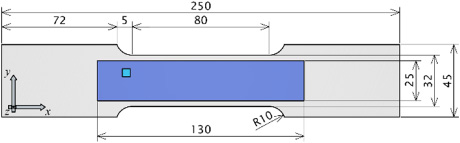
Sample view with dimensions.
Each sample was manually magnetized by moving the permanent magnet array in the direction of the y-axis with a speed of ca. 5 mm/s. Next, the residual magnetization was measured in the area shown in Fig. 1, utilizing an HMC 5883L magnetometer moved on the x- and y-axis. Subsequently, each sample was subjected to a different static stress level. An overview of the induced stress values gives the Table 1 underneath.
Samples and induced stress levels, along with elongations
After the tensile stress test, the measurement of the residual magnetization was repeated. Next, the two-dimensional data for the original and stressed samples were filtered using a fourth-order Butterworth digital filter and averaged to achieve one-dimensional signals. For the analysis, a couple of scanning paths were chosen to avoid the influence of the sample edges. Finally, signal parameters were evaluated.
Several signal cycles were chosen to calculate the signal frequency (1). Next, averaged peak-to-peak signal value was calculated using (2). In this case, the central part of the signal was used for calculations.
Using the parameters given by (1) and (2), relative mean changes in magnetic field induction (3) and magnetic field frequency (4) were calculated to evaluate residual magnetization variations in each sample after tensile stress tests.
The averaged, one-dimensional signals measured for three selected samples: S01 (elastic stress-induced changes), S04 (yield point), and S07 (plastic stress-induced changes) are presented in Fig. 3.
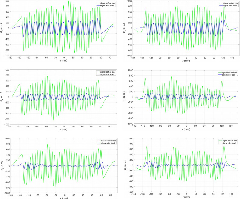
Magnetic field components measured before (green line) and after (blue line) stress-loading the samples; (a) B x for S01, (b) B z for S01, (c) B x for S04; (d) B z for S04, (e) B x for S07, (f) B z for S07. The abbreviation a.u. in the y-axis label stands for an arbitrary unit.
Based on Fig. 3, it can be concluded that the amplitude of the signal decreases with the increase in the stress level. It is especially evident in the middle part of the signals. In the case of sample S07, which belongs to the plastic region, the signal amplitude and frequency decreased drastically compared with the signal measured before the tensile stress test.
Changes in the magnetization of samples caused by stresses in the material and the accompanying deformations (of an elastic nature) can be explained by the tendency of the magnetic domains forming the magnetization pattern to the state with the lowest possible free energy. It is assumed that the material volume of interest before magnetization is in a stable energy state with a certain minimum free energy value. As a result of magnetization, the energy state changes (the energy of the analyzed sample volume increases) and reaches a new metastable level. At the level of the ferromagnetic crystal structure, it is done by the displacement and growth of the surface of the boundaries of the magnetic domains in accordance with the system of force lines of the field forcing the magnetization pattern. The stabilization of domain boundaries in metastable positions occurs due to blocking them on defects in the crystal structure of the material, such as vacancies, dislocations, or non-ferromagnetic inclusions. The deformation of the ferromagnetic crystal lattice caused by mechanical stresses to a greater or lesser extent, inactivates the places of immobilization of the domain boundaries. It allows for a spontaneous change of their position towards other metastable states with lower energy. It can be observed macroscopically as the changes in the sample’s magnetization pattern described in this work.
However, the assessment of the structural condition comprising only the analysis of signal variation may pose a problem due to the minor changes between two stress levels similar in value. In order to overcome this issue, additional graphs with relative mean change in the magnetic field and its frequency were prepared. Exemplary graphs are provided in Fig. 4.
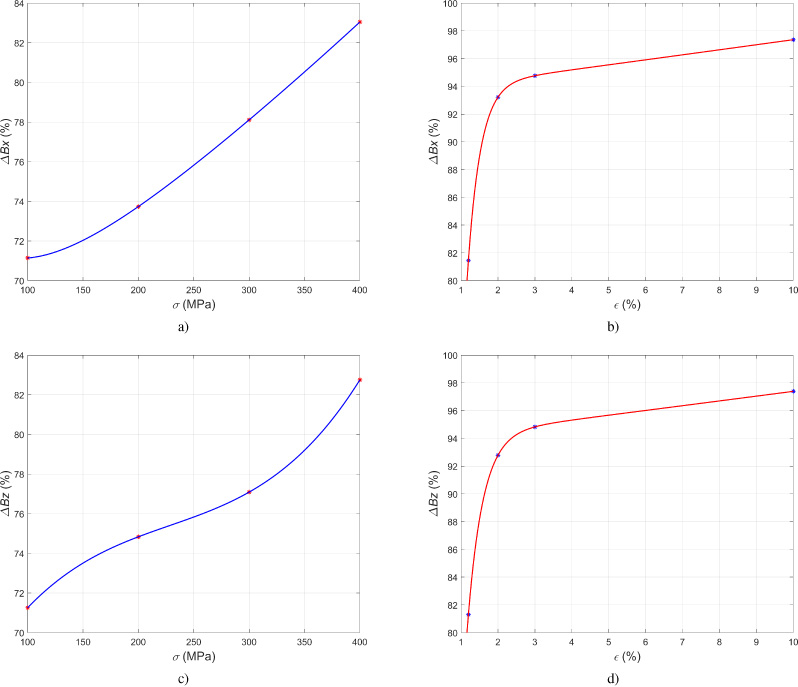
Relative mean changes of the magnetic field component; (a) ΔB x for S01-S04, (b) ΔB x for S04-S08, (c) ΔB z for S01-S04; (d) ΔB z for S05-S08.
As shown in Fig. 4, the relative mean change in the magnetic field in the elastic range increases nearly linearly for the x-component. In the case of the z-component, the curve also increases, but its shape resembles a cubic polynomial. In the plastic range beyond the yield point, which corresponds to the S05 sample, the relative mean change grows rapidly, and then, after passing the sample S07, the growth slows down. Compared with the elastic range, the curves for the plastic range increase exponentially. Due to the monotonicity of the curves, the stress level may be assessed unequivocally.
The results of the research, despite the novelty of the technique applied, may be referred to as satisfactory and perspective. The magnetic recording method can be a helpful nondestructive testing approach, enabling the stress level to be evaluated in a relatively straightforward and unambiguous way. This method does not need advanced data analysis algorithms because of the plain magnetization path shape (e.g., sinusoid-like). Nonetheless, further research should be conducted to determine the impact of the magnetizing process (e.g., automatic shifting of permanent magnet array instead of manual), data analysis algorithms selection, and the process of the residual magnetization measurement. Currently, additional research is being carried out to investigate how time affected magnetization paths recorded before three years.