Predicting of spatial electric field generated by substation switch operation based on AOS-GCN-LSTM Model

Abstract

The radiation of adjacent field sources has a specific spatial correlation. In order to suppress electromagnetic disturbance and improve the electromagnetic compatibility of secondary equipment, the electric field’s spatial coupling characteristics and distribution law should be mastered. Therefore, a method for predicting the spatial electric field generated by substation switching operation based on the Atomic Orbital Search-Graph Convolution Network- Long and Short-Term Memory (AOS-GCN-LSTM) model is presented to deal with this problem. First, the GCN is used to construct graph data according to node characteristics and topology information. The feature selection uses the Maximum Information Coefficient (MIC) to extract the spatial correlation of the adjacent field source radiation. At the same time, the LSTM is used to capture the temporal correlation characteristics of different position field strengths in space. Then, the AOS is used to optimize the model with a hyperparameter. In addition, the simulation data of the full-wave simulation model of the spatial electric field generated by switch operation in a 220 kV GIS substation is an example of verification. The results show that the prediction error of the proposed method is below 3%, and it has strong adaptability to the application environment and good prediction performance.

Keywords

Switch operation spatial electric field AOS-GCN-LSTM model full-wave simulation field strength prediction

1. Introduction

The intelligent development trend of substations has led to the gradual implementation of the on-site layout of secondary equipment [1]. Compared with traditional layout methods, electronic devices in this type of layout are in a more severe electromagnetic interference environment, especially facing intense spatial electromagnetic interference problems. Furthermore, switch operation is the essential electromagnetic interference source in substations, and its opening and closing will generate substantial radiation interference [2]. Studying the transient spatial electric field distribution characteristics of substations during switch operation can summarize the general rules of transient electric field distribution, providing a basis for the planning, construction, and equipment procurement and installation of intelligent substations.

Currently, there are three standard research methods for the radiation field in substations. These three methods are field measurement, numerical prediction, and laboratory physical simulation. The on-site measurement method is relatively easy. In recent years, many switch operation tests have been carried out domestically and internationally in GIS substations [3–6], and many research results have been achieved. However, this method is also most susceptible to the influence of other interference sources on site. As the electromagnetic environment of substations becomes more severe, measurement errors will gradually increase, making it difficult to accurately grasp the distribution pattern of electric fields caused by switch operation. The numerical prediction method and laboratory physical simulation method have high accuracy and solid theoretical validity in predicting field strength, which can better simulate the switching operating environment. During substation switching operation, Rao MM et al. studied the characteristics of the electromagnetic field amplitude near the casing based on the time-domain finite difference (FDTD) simulation model and compared the impact of switch position, whether there are metal buildings around on the electromagnetic radiation level [7]. A three-dimensional full-wave model [8,9] is established in the electromagnetic field software CST to simulate the fast transient electromagnetic field generated by GIS substation switch operation. However, the above research was conducted in a simple electromagnetic environment, and the actual electromagnetic environment is complex. The planning and design of substations often require a large amount of calculation, and the complexity of modeling and solving is exceptionally high. This makes it challenging to meet the engineering needs of three-dimensional electromagnetic field simulation based on physical model solving.

Intelligent learning algorithms have developed rapidly in recent years. Compared to other research methods, data-driven methods to extract the changes in spatial electric field data for the prediction can avoid many complex problems (such as structure, boundary conditions, voltage changes, and reducing the impact of other interference sources). Through literature research, it was found that there are appropriate methods for reference. However, there is no suitable solution for the problems proposed in this paper, and the accuracy and convergence of the relevant solutions could be higher. By studying the space electromagnetic field of a base station, a method of field strength prediction based on ray tracing and neural networks is proposed [10,11]. However, this method focuses on the accuracy of scene data acquisition. However, it needs to pay attention to the problem that neural network is easy to fall into local optimization for training samples, and the prediction error is significant. These studies provide a rich theoretical basis for researching intelligent algorithms in electromagnetic compatibility. The deep learning algorithm is the latest development in machine learning [12,13], which can extract data features at a deep level and better capture nonlinear relationships between data. LSTM can predict multiple steps from sequence to sequence [14]. However, the LSTM model cannot consider the spatial correlation of measurement points, resulting in low prediction accuracy of the model. GCN is based on the graph Fourier transform and Laplacian matrix [15], which can better extract the features of non-European spatial data. Xu G et al. proposed a spatiotemporal correlation GCN-LSTM prediction model but did not consider the impact of manually setting the hyperparameter of LSTM on the model [16].

Based on this, the spatial and temporal characteristics of the electric field were considered, and a method for predicting the spatial electric field strength of substation switching operation based on the AOS-GCN-LSTM model was present. This method first constructs graph data based on the characteristics and topology information of the field source nodes. The attenuation and coupling of field source radiation were considered, and the maximum information coefficient method was used for feature selection to realize the division of the coupling area. They were extracting spatial features of field source radiation using GCN. At the same time, the temporal and spatial correlation characteristics of field strength at different points in the space are captured using the LSTM, and the spatiotemporal prediction model of GCN-LSTM is designed accordingly to capture the spatiotemporal dependence of field strength. Then, AOS is used to optimize the hyperparameter of the model, and the spatial electric field prediction model of substation switch operation based on AOS-GCN-LSTM is constructed. Moreover, take the simulation data of the spatial electric field simulation model for switch operation in a 220 kV standard box GIS substation as an example to conduct research. The simulation results show that this method has good prediction accuracy. Compared with modeling and simulation, it has the advantages of short calculation time and fast convergence speed, providing a new method for predicting spatial electric fields.

2. Data processing and spatial electric field prediction algorithms

2.1. Data processing

The electric field strength with the concept of dynamic potential was combined, and a formula for calculating the tangential component of electric field strength generated by switch operation can be obtained, as shown in Eq. (1). $\begin{eqnarray}\boldsymbol{E}_{L}(\boldsymbol{r},t)=\frac{\partial \boldsymbol{A}_{L}(\boldsymbol{r},t)}{\partial t}+\partial {\varphi}(\boldsymbol{r},t)/\partial L\end{eqnarray}$ (1) where E _L( r , t) is the tangential component of the electric field strength of the wire L located at position r at time t; A _L( r , t) is the dynamic vector of the surface current of the wire L; φ ( r , t) is the dynamic scalar of the surface axis current of the wire L.

In free space, electric and magnetic fields excite each other. The motion law of the electromagnetic field will be derived from Maxwell’s equations in the passive case. The wave equation of the electric field can be obtained by taking the curl of the electric field equation, as shown in Eq. (2). $\begin{eqnarray}\displaystyle {\nabla}^{2}\boldsymbol{E}-\frac{1}{c^{2}}\frac{\partial ^{2}\boldsymbol{E}}{\partial t^{2}}=0\end{eqnarray}$ (2) where E is the strength of the spatial electric field, c is the propagation speed of the electromagnetic wave, and t is the propagation time.

In the substation, the switch operation takes place inside the GIS equipment. The electromagnetic interference received by the secondary equipment is leakage from the connection gap of the GIS equipment bushing or casing. For the calculation of the external spatial electric field of the equipment, it is not only necessary to consider the direction of the electric field but also the influence of fluctuations and the changes in the polarization and magnetization characteristics of the medium over time, boundary conditions, the refraction and reflection of electromagnetic waves inside the bushing, the loss of field strength over time and distance, and the coupling of multiple field sources. Therefore, no mature formula can directly solve its radiation field.

At present, the Finite Integral Technique (FIT) is often used to deal with the electric field in space. With this method, when the electromagnetic field changes rapidly with time, the induced magnetic field effect caused by its displacement current and the induced electric field effect caused by its magnetic field change cannot be ignored [11]. So Maxwell’s integral equation is shown in Eqs (3) and (4): $\begin{eqnarray}\displaystyle \text{} & \text{} & \displaystyle \oint _{l}\boldsymbol{H}\cdot dl={\gamma}\int _{s}\boldsymbol{E}\cdot dS+{\varepsilon}\int _{s}\frac{\partial \boldsymbol{E}}{\partial t}\cdot dS\end{eqnarray}$ (3) $\begin{eqnarray}\displaystyle \text{} & \text{} & \displaystyle \oint _{l}\boldsymbol{E}\cdot dl=-{\mu}\int _{s}\frac{\partial \boldsymbol{H}}{\partial t}\cdot dS\end{eqnarray}$ (4) where H represents the magnetic field strength, E is the electric field strength, 𝛾 is the conductivity, ϵ is the dielectric constant, and μ is the magnetic permeability.

The radiation characteristics of the field source, the field strength’s time-domain characteristics, and the switch operation’s spatial coupling characteristics can all be obtained using finite integral technology. However, this method has high requirements for the operating environment, and simulation modeling requires much time.

Note: circuit breaker (CB), isolation switch (DS), maintenance/fault closing grounding switch (ES/FES), bus (BUS), current transformer (CT), voltage transformer (VT), lightning arrester (LA), local control cabinet (LCP), cable terminal (CSE), SF6∖air Bsg (1M), 2M SF6∖oil Bsg (2M), circuit breaker mechanism (CBM).

Fig. 1.

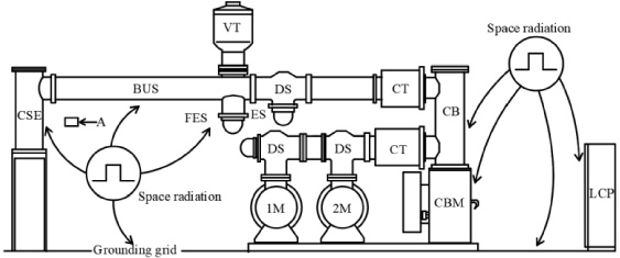
The coupling pathway of spatial electric field during switch operation.

As shown in Fig. 1, the transient electromagnetic wave usually radiates from the bushing or the gap between the casing and the casing to form spatial coupling. Therefore, the spatial electromagnetic fields at different points near GIS equipment can be regarded as being influenced by multiple field sources.

As shown in Fig. 2, this paper starts with the measurement data of the electric field. The radiation characteristics, time-domain characteristics of field strength, and coupling characteristics of the spatial electric field are obtained by model training. The data-driven electromagnetic field prediction method calculates the electric field strength in space and obtains the distribution law of the electric field strength. The commonly referred to as electric field strength refers to the maximum amplitude of the electric field, so research is conducted on the half wavelength of the maximum amplitude, as shown in Fig. 3.

Fig. 2.

Methods of electric field prediction.

Fig. 3.

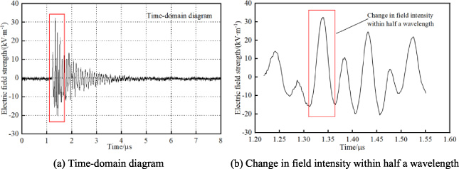
Time domain diagram of electric field strength.

In this paper, space coordinates and field strength are used as input data for electric field prediction. In order to keep the dimension of data consistent and make the model easy to train, the data are normalized, as shown in Eq. (5). $\begin{eqnarray}Z_{n}=\frac{Z-Z_{m}}{Z_{M}-Z_{m}}\end{eqnarray}$ (5) where Z is the actual data, Z_n is the normalized data, Z_M is the maximum value, and Z_m is the minimum value.

Equation (6) was used to de-normalize the data at the end of the model training. $\begin{eqnarray}Z=Z_{m}\cdot (Z_{M}-Z_{m})+Z_{M}.\end{eqnarray}$ (6)

2.2. Prediction algorithm of spatial electric field

2.2.1. Graph convolutional network

The basic idea of GCN [17] is to project the non-euclidean spatial data of electric field strength distribution affected by multiple excitation sources into Euclidean space. After the data is convoluted, the result is returned to a non-euclidean space. Its operation is based on the graph Fourier transform and Pierre-Simon Laplace matrix, which can better extract the spatial distribution characteristics of electric field strength.

Fig. 4.

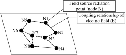
Field strength radiation distribution map.

At the t-moment, the spatial distribution of electric field strength near GIS equipment can be defined as a non-Euclidean spatial electric field graph G = (N, E, A, H), as shown in Fig. 4. Among them, N represents the node, which is the radiation point of the field source. Its adjacency matrix is A , which describes the radiation characteristics of the electric field; E represents the connection between nodes, i.e., the electric field coupling relationship between stations. If there is a connecting edge between two nodes, then the element in the adjacency matrix is 1; otherwise, it is 0; H represents the characteristic matrix of the node. Because each field source has its geometric parameters and radiation ability, the graph cannot be accurately expressed only by the adjacency matrix. The matrix value is the electric field strength data of the radiation point of the field source at t-moment. To avoid losing their information during the feature extraction process, self-connections are added to each node in the network. In the adjacency matrix, the element value from the node to itself is 1, and the element on the diagonal becomes 1. $\tilde{\boldsymbol{A}}$ represents the adjacency matrix with self-connection. The calculation formula for GCN is shown in Eq. (7). $\begin{eqnarray}\boldsymbol{H}^{(\boldsymbol{I}+1)}={\sigma}(\tilde{\boldsymbol{O}}^{-\frac{1}{2}}\cdot \tilde{\boldsymbol{A}}\cdot \tilde{\boldsymbol{O}}^{-\frac{1}{2}}\cdot \boldsymbol{H}^{\boldsymbol{I}}\cdot \boldsymbol{W}^{\boldsymbol{l}})\end{eqnarray}$ (7) where H ^{(
I
)} represents the eigenvector matrix of all stages in the l-layer, and H ^{(
I
+
1
)} represents all eigenvector matrices after one convolution operation. σ is the sigmoid activation function, W is the weight matrix, and A is the radiation field graph adjacency matrix. Moreover, $\tilde{\boldsymbol{A}}$ is the adjacency matrix with a self-connected network and $\tilde{\boldsymbol{A}}=\boldsymbol{A}+\boldsymbol{I}$ . $\tilde{\boldsymbol{O}}$ is the correlation matrix with self-connection; only the diagonal elements have values. The calculation formula for the self-connecting matrix is shown in Eq. (8). $\begin{eqnarray}\tilde{O} _{ii}=\mathop{\sum }_{j}\tilde{A}_{ij}.\end{eqnarray}$ (8)

The electric field’s attenuation and the field source’s influence on the measurement point were considered. The radiation of the field source with higher field strength and larger volume is more robust. Moreover, the distance between the measurement point and the field source will also impact the measurement point. Therefore, the MIC is used for feature selection, as shown in Eqs ((9)) and ((10)). Considering only the field source whose correlation to the field source is higher than 15%, if all of them are lower than 15%, the field source with the highest correlation is selected to simplify the calculation. By calculating the MIC between the field source and the measurement point, the spatial correlation between the field sources can be better characterized. $\begin{eqnarray}\displaystyle \text{} & \text{} & \displaystyle I[X;Y]=\mathop{\sum }_{X,Y}p(X,Y)\log _{2}\frac{p(X,Y)}{p(X)p(Y)}\end{eqnarray}$ (9) $\begin{eqnarray}\displaystyle \text{} & \text{} & \displaystyle MIC[x,y]=\max _{|X||Y|\lt B}\frac{I[X;Y]}{\log _{2}(\min (|X|,|Y|))}\end{eqnarray}$ (10) where I[X; Y] is the probability density function of Monte Carlo, p (X, Y) is the joint probability density distribution function, and |X | and |Y | is the number of segments divided in the X and Y directions, respectively. The total number of all squares is less than B, and B is an empirical value. Usually, it is taken to the power of 0.6 or 0.55 of the total data, and in this paper, it is taken as 0.6.

2.2.2. Long short term memory

LSTM is mainly used for processing sequential data [18]. It can effectively maintain the dependency relationship between data before and after and has a significant processing effect on time series. Considering that the time for the electric field to change within half a wavelength is too short, Eq. (6) is used for normalization. The spatial electric field strength of the measurement point within the wavelength is consistent with time series data, and there is a correlation between the current electric field strength of a measurement point and its previous electric field strength. Therefore, we can model the series data modeling according to the time dependence and extract the change characteristics of the time series data. LSTM selectively passes through information by introducing a gating mechanism, enabling it to add and delete cell information. Its unit structure is shown in Fig. 5.

Fig. 5.

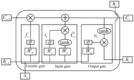
Schematic diagram of LSTM structure.

One LSTM unit consists of three gates, namely a forgetting gate (f_t), memory gate (i_t), and output gate (o_t). The formulas are shown in Eqs (11), (12), (13), (14), (15), and (16). When there is no helpful information in the input sequence, the value of the forgetting gate (f_t) will approach 1, and the value of the input gate (i_t) will approach 0 so that past helpful information will be saved. When there is the leading information in the input sequence, the value of the forgetting gate (f_t) approaches 0, and the value of the input gate (i_t) approaches 1. At this point, the LSTM model forgets the past memory and records the main memory. The design of LSTM output (h_t) is jointly controlled by forgetting gates, output gates, input gates, and internal memory units, enabling the entire network to grasp the relationships between sequence information better.

Forgetting gate, filtering the degree of forgetting the unit state at the previous moment. $\begin{eqnarray}f_{t}={\sigma}(W_{f}\cdot [h_{t-1},x_{t}]+b_{f}).\end{eqnarray}$ (11)

Input gate to determine which information is added to this unit. $\begin{eqnarray}i_{t}={\sigma}(W_{i}\cdot [h_{t-1},x_{t}]+b_{i}).\end{eqnarray}$ (12)

At time t, the unit status is updated, and new memory information is selectively recorded in C_t based on f_t and i_t. $\begin{eqnarray}\displaystyle \text{} & \text{} & \displaystyle \tilde{C}_{t}=\tanh (W_{c}\cdot [h_{t-1},x_{t}]+b_{c})\end{eqnarray}$ (13) $\begin{eqnarray}\displaystyle \text{} & \text{} & \displaystyle C_{t}=f_{t}\cdot C_{t-1}+i_{t}\cdot \tilde{C}.\end{eqnarray}$ (14)

At time t, the output gate activates C_t and determines the output size of C_t. $\begin{eqnarray}\displaystyle \text{} & \text{} & \displaystyle o_{t}={\sigma}(W_{o}\cdot [h_{t-1},x_{t}]+b_{o})\end{eqnarray}$ (15) $\begin{eqnarray}\displaystyle \text{} & \text{} & \displaystyle h_{t}=o_{t}\cdot \tanh (C_{t})\end{eqnarray}$ (16) where W_f, W_i, W_c, and W_o represent the weight matrix of the LSTM unit on the electric field strength at the current time. b_f, b_i, b_c, and b_o represent the bias matrix of the LSTM unit for field strength information at the current time. The x_t represents the electric field strength at the current time. C_t−1 and C_t are the LSTM unit state information at time t −1 and time t. $\tilde{C}_{t}$ are the LSTM state update information at time t. The h_t−1 and The h_t are the LSTM state information at time t −1 and time t, respectively. σ is the sigmoid activation function, and tanh is the hyperbolic tangent activation function. f_t, i_t, and o_t are the control coefficients of the three LSTM gate structures, respectively.

2.2.3. Atomic orbital search

AOS is an intelligent optimization algorithm based on some principles of quantum mechanics and the quantum atomic model [19]. The algorithm describes the optimal solution by the lowest level of the electron transition in the atomic orbital. Multiple particles in the algorithm’s search space search for the global solution by sharing individuals and the optimal global position. This avoids the problem of falling into local optima when single-particle algorithms search for global solutions. Compared to other optimization algorithms, it can achieve high convergence without any improvement. Like other neural network models, the GCN-LSTM model parameters must be set manually. These parameters control the network structure of the prediction model. The prediction effect of models with different parameters has a considerable gap. Therefore, the parameter information of the GCN-LSTM model is associated with the electronic information of AOS for hyperparameter optimization.

In AOS, electrons are defined as candidate solutions (X), and the initialization of each candidate solution is randomly determined by Eq. (17). $\begin{eqnarray}\displaystyle x_{i}^{j}(0)=x_{i,\min }^{j}+\mathit{rand}\cdot (x_{i,\max }^{j}-x_{i,\min }^{j}),\left\{\begin{array}{@{}l@{}}i=1,2,\ldots ,m\quad \\ i=1,2,\ldots ,d\quad \end{array}\right. & & \displaystyle\end{eqnarray}$ (17) where $x_{i}^{j}$ (0) represents the initial position of the candidate solution, $x_{i,\min }^{j}$ and $x_{i,\max }^{j}$ are the minimum and maximum bounds of the j-th decision variable of the i-th candidate solution. Rand is a uniformly distributed random vector within the range of [0,1], and m is the total number of candidate solutions in the search space.

Each electron’s energy state is considered the candidate solution’s objective function value in the mathematical model. Candidate solutions with better objective function values represent electrons with lower energy levels, while electrons with higher energy levels are only considered when they have worse objective function values.

2.3. AOS-GCN-LSTM spatial electric field prediction model

Due to the attenuation of the radiation from the field source, the field strength of the measurement point is only affected by a single field in a certain area. In order to reduce the algorithm’s complexity and improve the training accuracy, the maximum information coefficient is used for area division in this paper. Due to the influence of the radiation from nearby field sources on the field strength of the measurement point in the coupling area, GCN is used to extract the spatial radiation characteristics of the electric field strength at various times during the wavelength period and the correlation between various field sources. The spatial electric field eigenvalues calculated by GCN at each time point are used as inputs to the LSTM, thereby achieving spatial and temporal coupling and predicting electric field strength in various areas within the boundary range.

In nonparametric methods, LSTM has a solid nonlinear fitting ability. However, the setting of model hyperparameters often depends on experience or multiple experiments, which significantly impacts the efficiency of model training. Therefore, this paper proposes an AOS-GCN-LSTM model based on the spatiotemporal correlation graph structure of spatial electric field strength data and electric field measurement points connected by an AOS-optimized GCN-LSTM network. When predicting the spatial electric field intensity, the LSTM model is trained by using the electric field intensity data extracted by GCN, which can make the two models complementary and obtain better prediction effects. The AOS-GCN-LSTM algorithm proposed in this paper is shown in Fig. 6. The parameters of the GCN-LSTM model are optimized by the AOS algorithm, and the GCN-LSTM model is constructed to predict the electric field intensity. Among them, GCN extracts the features of each site through aggregation, update and circulation, and the LSTM uses the superposition of two LSTM networks to model the time series data. At the same time, the model consists of a decoder and an encoder [20]. The encoder embeds GCN into LSTM, uses GCN to learn the network structure of cell state C and hidden state h of the field source at each moment, and uses LSTM to learn the time information of each station and radiation area. The decoder is a completely connected layer, which maps the extracted features back to the original space. Finally, the prediction network is output to realize the spatial electric field intensity prediction of the network.

Fig. 6.

Flow chart of AOS-GCN-LSTM algorithm.

The specific running steps of the AOS-GCN-LSTM algorithm are as follows.

Step 1: Firstly, the coordinates of each measurement point and the electric field strength of each station at time t are input into the convolutional neural network of the graph to extract the spatial relationship between stations. Then, the experimental data is divided into training and testing sets, and the data is normalized. The ratio of the training set to the test set is 8:2.

Step 2: Initialize the model. The number of hidden layer units, learning rate, iterations, network layers, learning time step, data training batch, and the number of neurons in the model is taken as optimization objects. And AOS is initialized.

Step 3: Calculate the fitness value of the electron according to the optimal global value of the electron. The mean square error (MSE) is selected as the evaluation standard and the fitness value of each electron.

Step 4: Equation (18) is used to update the position of the electron group to calculate the current electron position $X_{i+1}^{k}$ , and record it. $\begin{eqnarray}\displaystyle X_{i+1}^{k}=X_{i}^{k}+\frac{{\alpha}_{i}\times ({\beta}_{i}\times LE-{\gamma}_{i}\times BS)}{k},\left\{\begin{array}{@{}l@{}}i=1,2,\ldots ,p\quad \\ k=1,2,\ldots ,n\quad \end{array}\right. & & \displaystyle\end{eqnarray}$ (18) where $X_{i}^{k}$ and $X_{i+1}^{k}$ are the current and future positions of the i-th candidate solution in the k-th layer; LE is the candidate solution with the lowest energy level in an atom; BS is the binding state of atoms; 𝛼_i, 𝛽_i and 𝛾_i is a vector containing randomly generated numbers uniformly distributed in (0,1) to determine the energy released.

Step 5: When the iteration is completed, or the best position is found, the termination condition is satisfied, and the optimal hyperparameters are obtained. If not, return to step 3 and iterate again.

Step 6: Building GCN-LSTM model with optimal hyperparameters.

Step 7: GCN extracts features based on the maximum information coefficient.

Step 8: The processed data are input into the LSTM model and trained to output the final prediction result.

3. Example analysis

3.1. Simulation design

Due to the limitations of actual measurement conditions, to verify the AOS-GCN-LSTM model’s predictive effect, a 220 kV GIS substation switch operation simulation [21] was established to obtain training sample data. The full-wave simulation model is modeled by CST electromagnetic simulation software and simulated by a time domain solver. In this paper, the calculation method of space electric field strength is to take fast transient overvoltage as the excitation source of space electromagnetic disturbance. According to the physical characteristics and geometric parameters of the objects in the actual layout near the substation switch, the calculation model of the boundary value problem of the electric field is established. The spatial electric field distribution is obtained by using the full-wave numerical calculation method of the time-domain electromagnetic field. From the point of view of model structure simplification and algorithm simplification, the complexity of the model is reduced at different levels to improve the calculation efficiency, and the deviation degree of the calculation results is monitored at the same time so that a simplified model with both calculation efficiency and effectiveness is obtained by comparison. The experimental and simulation errors were considered; the method can accurately calculate and obtain the transient electromagnetic field pulse waveform. Taking 220 kV GIS Substation as an example, its typical switch operation is shown in Fig. 7(a). Circuit breakers and isolation switches achieve the switching operation of busbars and lines. A 220 kV GIS substation switch operation simulation model is established, as shown in Fig. 7(b), which is solved by the finite integral technique. The 220 kV substation is an outdoor structure with a design-rated voltage 252 kV and a rated current of 3150 A. When modeling GIS, it is necessary to consider the impact of factors such as grounding grid and bracket grounding on the distribution of electromagnetic fields. The structure and relative positions of the GIS shell, central conductor, support, and grounding grid are all established according to the GIS drawings. The GIS shell is connected to the grounding grid through brackets and grounding strips. The bushing is made of porcelain, with a vertical cylindrical inner wall and circular outer wall. The electromagnetic characteristic parameters of the materials used are shown in Table 1.

Table 1
Electromagnetic characteristics of materials used in modeling

Model structure Relative dielectric constant ϵ Conductivity δ (S/m)

GIS casing, center guide rod, overhead line, flange, support structure (aluminum) – 3.56 × 10⁷

Grounding grid (copper) – 5.96 × 10⁷

Bushing (porcelain) 6 1.00 × 10⁻¹⁵

Ground 1 1.00 × 10⁻²

Model structure	Relative dielectric constant ϵ	Conductivity δ (S/m)
GIS casing, center guide rod, overhead line, flange, support structure (aluminum)	–	3.56 × 10⁷
Grounding grid (copper)	–	5.96 × 10⁷
Bushing (porcelain)	6	1.00 × 10⁻¹⁵
Ground	1	1.00 × 10⁻²

Fig. 7.

Schematic diagram of GIS substation switch operation simulation.

To verify the accuracy of the full wave simulation model, this model was used to measure the transient shell voltage of a 220 kV gas-insulated substation. “VFF” stands for over-voltage between insulating flanges. Compared with existing measurement data [22], the simulation and measurement results of VFF have good consistency in characteristic waveform parameters such as amplitude, rise time, pulse duration, and main frequency, indicating the correctness of full wave simulation. The parametric statistics of the VFF micropulse waveform are shown in Table 2.

Table 2

Parametric statistics of VFF micropulse waveform

Observation point	Peak value (kV/m)			Single pulse duration t_d ∕μs	Peak rise time t_r ∕μs	Main frequency/MHz
	Maximum value	Minimum value	Peak-to-peak
Simulation 1	8.1	−7.3	15.4	5	0.0177	4.2, 6.3, 9.4, 20.
Simulation 2	5.4	−4.6	10	5	0.0133	4, 7.1, 11.2, 21.7
Measurement 1	7.8	−6.8	14.6	5	0.0179	4.6, 6.4, 8.2, 21
Measurement 2	4.9	−4.2	9.1	5	0.0144	4.6, 6.8 11.8, 22

By observing the simulation model, it can be seen that electromagnetic waves leak from multiple locations. Moreover, during on-site measurement, not only cannot the leak location be fully grasped, but the measurement conditions are also limited. Therefore, in the numerical analysis of this paper, four locations with severe electromagnetic leakage were selected as the field sources, while other locations were assumed to have no electromagnetic leakage for prediction research. In order to verify the accuracy of the simulation method, the electric field in the position with serious electromagnetic leakage is measured. Wherein each measuring point is gradually away from the field source in units of 10 cm. Figure 8 shows the comparison between the measured data and simulated data. According to the analysis results, the error is less than 8%. The model can simulate the radiation characteristics of the electric field during switch operation. Through the simulation calculation, the lack of measured data can be made up. At the same time, the focus of this paper is to propose a method to predict the spatial electric field of the substation, and the simulation data is only to verify the accuracy of the method.

Fig. 8.

Comparison between simulated values and measured values of measuring points in different measuring areas.

3.2. Model parameter settings

The model parameters mainly include learning rate, number of iterations, the proportion of random neuron inactivation, number of network layers, learning time steps, data training batches, and number of neurons. Different parameter settings can greatly affect prediction accuracy. In order to reduce the influence of human factors, the value range of the optimized hyperparameter is set as follows: the hidden layer is set as two layers, The adma function is used as the optimization function, and the MSE function is used as the loss function [18]. The complexity of the data fitted by the model determines the number of network layers. In order to prevent the network model from over-fitting, dropout regularization was used to deal with it. The range of the network hyperparameter is set as follows: the range of learning rate is (0.001, 0.01), the range of training times is (10,100), the number of neurons in the first hidden layer is (1,100), and the number of neurons in the second hidden layer is (1,100). At the same time, AOS is used for hyperparameter optimization. The AOS parameters are: the number of populations is 30, the maximum iteration is 100, the number of layers around the nucleus is 5, and the photon rate is 0.1. The hyperparameter optimization results are shown in Table 3.

Table 3
Hyperparameter optimization results

Learning rate Epoch Hidden node 1 Hidden node 2 Batch size

0.078 64 68 54 86

Learning rate	Epoch	Hidden node 1	Hidden node 2	Batch size
0.078	64	68	54	86

In order to evaluate the performance of the model, this paper uses mean absolute percentage error (MAPE), root mean square error (RMSE), relative error (RE), mean absolute error (MAE), and relative error curve as evaluation criteria to evaluate the error of the prediction results of the model [23]. When the model’s MSE, RMSE, MAE, and MAPE values are lower, and the relative error approaches zero, the model’s prediction accuracy is higher.

The results were compared with three other learning models, LSTM, CNN-LSTM, and GCN-LSTM. The training errors of the models are given in Table 4. In model training, the AOS-GCN-LSTM training error results were smaller than the corresponding models in the four indicators of MAPE, RMSE, MAE, and MSE. This paper proposes a model that reduces MAPE, RMSE, MAE, and MSE by 37%, 58%, 40%, and 65%, respectively, compared to the CNN-LSTM model. Compared to the GCN-LSTM model, the model reduces MAPE, RMSE, MAE, and MSE by 42%, 70%, 50%, and 74%, respectively. The AOS avoids the problem of quickly falling into local optima, achieves better parameters, and thus achieves better prediction performance.

Table 4

Training errors of different models

Model	MAPE	RMSE	MAE	MSE
LSTM	0.0873	0.4621	0.2936	0.2912
CCN-LSTM	0.0573	0.3036	0.1314	0.1217
GCN-LSTM	0.0518	0.2236	0.1104	0.0913
AOS-GCN-LSTM	0.0328	0.0943	0.0658	0.0324

Due to the radiation and spatial characteristics of the field source, only LSTM is used for prediction, resulting in relatively small measurement errors in a single field source area. However, in the coupling area of multiple field sources, the prediction error is relatively large due to the influence of other field sources. Using GCN to extract field strength features avoids the three-dimensional processing steps of CNN for two-dimensional images and can better obtain field strength features. Compared with CNN-LSTM and GNN-LSTM models without optimization algorithms, using parameter optimization algorithms can enable the model to obtain better network parameters, overcome the difficulties of traditional models in parameter selection, and improve prediction accuracy. The AOS used in this paper is a global optimization algorithm that is not easily trapped in local optima, resulting in better network parameters and improved model prediction accuracy.

3.3. Numerical tests of the algorithm

In this paper, the simulation data of switching operation in 220 kV GIS substation is used as the training data of the forecasting model. The data set takes 1,000 samples within half a wavelength. The data set is divided into training sets and test sets, which contain 800 and 200 samples respectively. Each sample consists of measuring time t, three-dimensional coordinates (x_t, y_t, z_t), and electric field intensity E_t. Among them, the training set data are the measurement time t_a, three-dimensional coordinates (x_ta, y_ta, z_ta) and electric field intensity E_ta of the measurement point, and the three-dimensional coordinates (x_tb, y_tb, z_tb) and electric field intensity E_tc of the secondary equipment layout point, and the input data of the test set data are the measurement time t_c, three-dimensional coordinates (x_tc, y_tc, z_tc) and electric field intensity E_tc of the measurement point. And the three-dimensional coordinates (x_td, y_td, z_td) of the secondary equipment layout point, and the output is the electric field intensity E_td of the secondary equipment layout point, and the research is carried out with MATLAB 2020a as the simulation platform.

From Figs 9 and 10, it can be concluded that after 50 iterations, the accuracy of the test set is gradually stable, indicating that the neural network is gradually convergent, and the loss value of the training set is gradually decreasing, with the minimum loss value of 0.4. It shows that the training effect of using a neural network model is good.

Fig. 9.

Change of accuracy of prediction model test set.

Fig. 10.

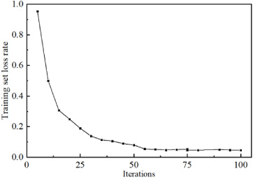
Loss value of training set of prediction model.

Meanwhile, the number of field sources and the distribution is more extensive on-site. Based on the existing, the impact of different field source numbers on measurement points was analyzed. Two schemes were designed to verify the predictive accuracy of the model. The first scheme is to select different measurement areas, each affected by single or multiple field sources, and predict the spatial electric field in different affected areas, as shown in Fig. 11. From Fig. 12, the prediction accuracy remains within 3% as the number of field sources increases. However, as the number of field sources increases, the stability of the prediction slightly decreases.

Fig. 11.

Prediction of field strength in different areas.

Fig. 12.

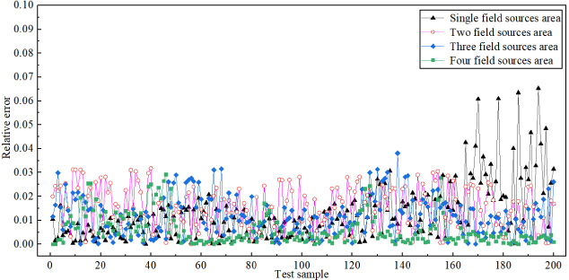
Relative error of field strength prediction in different areas.

The second scheme is to study a particular measuring area. Taking forecast area B as an example, the impact of the number of field sources on the prediction of space electric field is considered respectively. As can be seen from Fig. 13, the prediction using a single field source has a significant measurement error. The measured values are more accurate with the increase in the number of field sources. When three field sources and four field sources are used for prediction, the measured errors are not much different, and all are in good agreement with the simulated values. For a single field source, the error of some points is significant, possibly due to the coupling effect of other sources and the influence of model structure on the measured values.

Fig. 13.

Spatial electric field prediction based on different number of field sources.

This paper considers the impact of measurement location and model structure on measurement results. Three influence areas of field sources were selected, and three positions, namely forecast areas A, B, and C, were selected to analyze the predictive effect of the model. The prediction effect of the spatial electric field at different positions is shown in Fig. 14. From Fig. 15, it can be seen that under relatively open conditions, the model has good prediction results for the electric field strength. When there are obstacles, it will affect the measurement results. Therefore, increasing constraint conditions can be considered to reduce prediction errors.

Fig. 14.

Prediction comparison of spatial electric field strength at different areas.

Fig. 15.

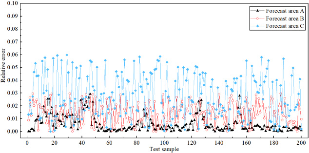
Prediction error of spatial electric field strength at different positions.

In this paper, the quality of the proposed prediction network is verified by using the existing field-measured data as training data. As shown in Fig. 16, the test results show that the prediction error is less than 7%, and the prediction error of measured data is slightly higher than that of simulated data. The first reason is that the measured value itself is inaccurate due to the influence of field conditions, and the second reason is that there are too few measured data, so the training of the network is not ideal. However, by forecasting the simulation data and measured data, it is proved that the model proposed in this paper has a certain practical reference value.

Fig. 16.

Comparison between measured value and predicted value.

4. Conclusion

In order to solve the problem of high computational complexity and modeling complexity in substation planning and design, this paper proposes a spatial electric field strength prediction method based on the AOS-GCN-LSTM model for switch operation based on a deep learning algorithm. GCN can extract spatial distribution features, LSTM can obtain temporal dependencies, and AOS can optimize the hyperparameter of the GCN-LSTM model. The effectiveness of the proposed method was verified through a comparison of full-wave simulation data of switch operation, and the main conclusions are as follows.

(1) The simulation and measurement results of VFF have good consistency in characteristic waveform parameters such as amplitude, rise time, pulse duration, and primary frequency, indicating the correctness of full wave simulation.

(2) The AOS-GCN-LSTM model is used to predict the spatial electric field strength, which can simultaneously learn the distribution characteristics of the field source and the time series characteristics of the electric field change of the measuring point. Compared with the traditional machine learning algorithm for Euclidean data, it has the advantages of high accuracy and no need for characteristic equations. The AOS has excellent global optimization characteristics and convergence speed. It not only avoids the artificial hyperparameter setting of the model but also improves the prediction accuracy.

(3) This paper not only considers the prediction accuracy of the algorithm under the influence of different numbers of field sources in a certain area but also considers the prediction accuracy of the algorithm for different positions under the influence of the same field source. As the number of field sources increases, the accuracy of prediction significantly improves, and the prediction stability slightly decreases but still maintains within a controllable range. In open areas, the measurement position has little effect on prediction accuracy. When there is a shelter, it will have a significant impact on the measurement results.

The prediction method proposed in this paper verifies the accuracy of the prediction method by taking the spatial electric field intensity produced by 220 kV GIS substation as an example. It is worth noting that the prediction method proposed in this paper is used to deal with the problem of strong spatial-temporal correlation, not only for characteristic objects but also for a wider range of inspected objects. At the same time, this paper finally predicts the measured data, which proves that the model proposed in this paper has a certain practical reference value.

Footnotes

Acknowledgements

This work was supported by the Basic Scientific Research Projects of Universities in Liaoning Province (Youth Project) (LJKQZ2021080).

References

Topolsky

D.V.

Topolskaya

I.G.

and Topolsky

N.D.

, Development of an intelligent measuring system for digital substations, in: 2018 International Multi-Conference on Industrial Engineering and Modern Technologies (FarEastCon); Vladivostok, Russia, 2018, Oct 3–4; Vladivostok, Russia, IEEE, 2019, pp. 1–4. doi:10.1109/FarEastCon.2018.8602868.

Guishu

Huijuan

Huaying

, Calculation of transient radiation field from metallic enclosure of GIS based on surface-patch model, IEEE Transactions on Magnetics42(4) (2006), 855–858, doi:10.1109/TMAG.2006.871384.

Barrack

C.S.

Siew

W.H.

and Pryor

B.M.

, The measurement of fast transient electromagnetic interference within power system substations, in: Proceedings of the 6th International Conference on Developments in Power System Protection, 1997 Mar 25–27, UK Nottingham, IET, 1997, pp. 270–273. doi:10.1049/cp:19970079.

Carsimamovic

Bajramovic

Ljevak

Very fast electromagnetic transients in air insulated substations and gas insulated substations due to disconnector switching, in: 2005 International Symposium on Electromagnetic Compatibility, 2005. EMC 2005, 2005 Aug 8–12, IEEE, Chicago, IL, USA, 2005, pp. 382–387. doi:10.1109/ISEMC.2005.1513544.

Jianfei

Lihui

Yubo

Experimental analysis of EMC immunity for field installed intelligent equipment, of intelligent substation, in: 2014 China International Conference on Electricity Distribution (CICED), 2014, Sept 23–26, IEEE, Shenzhen, China, 2014, pp. 1556–1564. doi:10.1109/CICED.2014.6991968.

Hengtian

Xiang

Xiaofan

, Characteristics of electromagnetic disturbance for intelligent component due to switching operations via a 1100 kV AC GIS test circuit, IEEE Transactions on Power Delivery32(5) (2016), 2228–2237, doi:10.1109/TPWRD.2016.2600277.

Rao

M.M.

Thomas

M.J.

and Singh

B.P.

, Electromagnetic field emission from gas to-air bushing in a GIS during switching operations, IEEE Transactions on Electromagnetic Compatibility2(49) (2007), 313–321, doi:10.1109/temc.2007.893334.

Binxian

Yuxin

Xiaohua

, 3D full maxwell research for effect of initial electromagnetic field on very fast transient overvoltage in GIS, IEEE Transactions on Dielectrics and Electrical Insulation23(6) (2016), 3319–3327, doi:10.1109/TDEI.2016.005390.

Smajic

Holaus

Kostovic

, 3D full-Maxwell simulations of very fast transients in GIS, IEEE Transactions on Magnetics47(5) (2011), 1514–1517, doi:10.1109/TMAG.2010.2090653.

10.

Vilovic

Burum

and Sipus

, A comparison of neural network models for indoor field strength prediction, in: ELMAR 2007, Sept 12–14, IEEE, Zadar, Croatia, 2008, pp. 251–254. doi:10.1109/ELMAR.2007.4418842.

11.

Wengang

Yumei

and Jinsheng

, Hybrid prediction model for field strength with ray tracing and artificial neural networks, in: IEEE 14th International Conference on Communication Technology, 2012, Nov 9–11, IEEE, Chengdu, China, 2013, pp. 301–305. doi:10.1109/ICCT.2012.6511233.

12.

Fengbo

Mengning

Wenyuan

, An efficient time-domain electromagnetic algorithm based on LSTM neural network, IEEE Antennas and Wireless Propagation Letters20(7) (2021), 1322–1326, doi:10.1109/LAWP.2021.3079313.

13.

Shrestha

and Mahmood

, Review of deep learning algorithms and architectures, IEEE Access (2019), 53040–53065, doi:10.1109/ACCESS.2019.2912200.

14.

Ghimire

Deo

R.C.

Wang

, Stacked LSTM sequence-to-sequence autoencoder with feature selection for daily solar radiation prediction: a review and new modeling results, Energies15(3) (2022), 1061, doi:10.3390/en15031061.

15.

Zijia

Yaoming

and Wenxin

, Evolution-driven randomized graph convolutional networks, IEEE Transactions on Systems, Man, and Cybernetics: Systems52(12) (2022), 7516–7526, doi:10.1109/TSMC.2022.3158276.

16.

Jianfeng

and Mingzheng

, The research of resource allocation method based on GCN-LSTM in 5G network, IEEE Communications Letters27(3) (2023), 926–930, doi:10.1109/LCOMM.2022.3224213.

17.

Kipf

T.N.

and Welling

, Semi-supervised classification with graph convolutional networks. arXiv preprint arXiv: 1609.02907. 2016. doi:10.48550/arXiv.1609.02907.

18.

Hochreiter

and Schmidhuber

, Long and short-term memory, Neural Computation9(8) (1997), 1735–1780, doi:10.1162/neco.1997.9.8.1735.

19.

Azizi

, Atomic orbital search: A novel metaheuristic algorithm, IEEE Applied Mathematical Modelling93 (2021), 657–683, doi:10.1016/j.apm.2020.12.021.

20.

Jinjin

Xueke

and Xuanheng

, GC-LSTM: graph convolution embedded LSTM for dynamic network link prediction, Applied Intelligence52 (2021), 7513–7528, doi:10.1007/s10489-021-02518-9.

21.

Fubin

Jianfei

Zhanpeng

Full wave simulation of transient electromagnetic field during switching operation of GIS power substation, in: Proceedings of the 4th International Conference on Electrical Engineering and Control Technologies (CEECT), 2022, Dec 16–18, IEEE, Shanghai, China, 2022, pp. 685–690. doi:10.1109/CEECT55960.2022.10030155.

22.

Yuanjia

Yangguan

and Weidong

, Measurement of transient enclosure voltage in a 220 kV gas insulated substation, in: 2015 IEEE International Instrumentation and Measurement Technology Conference (I2MTC) Proceedings, 2015, May 11–14, IEEE, Pisa, Italy, 2015, pp. 115–120. doi:10.1109/I2MTC.2015.7151250.

23.

Obiora

C.N.

Ali

and Hasan

A.N.

, Efficient method of finding the best time interval for predicting short term solar radiation using CNN-LSTM model, in: Proceedings of the 11th International Conference on Power Science and Engineering (ICPSE), 2022, Sept 23–25, IEEE, Eskisehir, Turkey, 2022, pp. 159–163. doi:10.1109/ICPSE56329.2022.9935441.