Coupled electric circuits method applied to pulsed eddy current NDT problem

Abstract

The present work concerns the study of the effect of variation of the thickness of 2D cylindrical test-piece and lift-off (the air gap between the sensor and the test-piece) on the sensor response in case of transient source current. The coupled circuit’s method employed is based on the mutual’s inductances calculation and with the association to Kirchhoff laws it yields to a transient algebraic equations system which is solved at each time step. The method is applied to the study of the pulsed eddy currents in cylindrical and axisymmetric device with electrical conductivity and geometrical dimensions variations.

Keywords

Coupled electric circuits pulsed eddy current non destructive testing and evaluation geometry and physical properties lift-off

1. Introduction

The Pulsed eddy current (PEC) technique differs from conventional eddy current testing in that the probe is excited by transient signal, rather than a sinusoidal waveform because of its rich variety of frequency [1].

As the consequence of many advances in electromagnetic nondestructive evaluation (NDE), pulsed eddy-current (PEC) technique has become more applicable and preferred for multi-defects detection and analysis [1,2]. The eddy currents sensors are used in several industrial applications which concern the evaluation of defect shape, test-piece thickness, physical properties of materials, defect detection in a piece and so… [2–5].

Numerical methods as finite elements, finite volumes are often used in the study of the defects detection using eddy currents non destructives techniques and also the non destructive evaluation for physical or geometrical characteristics identifications [2,7]. These methods are much time consuming for the resolution of the problems when small air-gaps or a thin layers occurs, such as conductive or ferromagnetic coatings. The latter induces prohibitive resolution time and in 3D problems modeling.

The present work proposes the use of coupled circuit’s method developed using Matlab package in order to study the effects of the thickness, the electrical conductivity and the lift off variations on the probe response. The method was used earlier for modeling induction heating devices, using as unknown the magnetic vector potential. [8] and non destructive testing or evaluation systems, by considering electromagnetic quantities unknowns [9]. The non destructive device is a 2D cylindrical and axisymmetric one and constituted of a probe which consists of a single coil at the inner of the hollow cylinder with high conductivity (Fig. 2). The voltage source of the sensor is considered as a pulsed square wave.

Fig. 1.

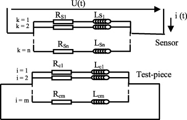
Equivalent electrical circuit (sensor with test-piece).

Fig. 2.

Half of the axisymmetric device.

2. Coupled electric circuits model

The coupled circuits method [6,8,9] uses a discretization of the domain in elementary coils. In the current study the method exploits an integral calculus for the evaluation of the electromagnetic quantities from the mutual inductances [6] instead of magnetic vector potential [8] or coupled electromagnetic quantities [9]. This process allows expressing the resistance of every elementary coil, the self-inductance and the mutual inductances between the various elementary coils.

The Kirchhoff’s laws applied to equivalent electrical circuit given by Fig. 1 allow us to write, for both the sensor and the test-piece (Fig. 2), the corresponding electrical equations (1) and (2) respectively: $\begin{eqnarray}\displaystyle U & = & \displaystyle R_{k}\cdot I_{k}+L_{k}\cdot \frac{dI_{k}}{dt}+\mathop{\sum }_{q=1\atop q\neq k}^{n}M_{kq}\cdot \frac{dI_{q}}{dt}+\mathop{\sum }_{i=1}^{m}M_{ik}\cdot \frac{dI_{i}}{dt}\end{eqnarray}$ (1) $\begin{eqnarray}\displaystyle 0 & = & \displaystyle R_{i}\cdot I_{i}+L_{i}\cdot \frac{dI_{i}}{dt}+\mathop{\sum }_{j=1\atop j\neq i}^{m}M_{ij}\cdot \frac{dI_{j}}{dt}+\sum _{k=1}^{n}M_{ik}\cdot \frac{dI_{k}}{dt}.\end{eqnarray}$ (2)R_i, L_i and I_i; R_k, L_k and I_k are the resistance, self-inductance and current (i and k are related to test-piece and inductor respectively). M_ij, M_ik, and M_kq are mutual inductances between i, j, k and q ⋅ I_i and I_j are currents in elements i and j (test-piece). I_k and I_q are currents in elements k and q (inductor) respectively. U is the applied voltage.

The mutual inductances between the different coils [8], the self-inductance and the resistance of every elementary coil, are given by Eqs (3), (4) and (5) as follow [6]: $\begin{eqnarray}\displaystyle M & = & \displaystyle {\mu}\cdot \sqrt{r_{1}r_{2}∼\cdot }∼\left[\left(\frac{2}{k}-k\right)\cdot K(k)-\frac{2}{k}\cdot E(k)\right]\end{eqnarray}$ (3) $\begin{eqnarray}\displaystyle L & = & \displaystyle {\mu}∼\cdot a∼\cdot \left(\ln \frac{8\cdot a}{d}-1.75\right)\end{eqnarray}$ (4) $\begin{eqnarray}\displaystyle R & = & \displaystyle {\rho}\cdot \frac{\ell }{s}\end{eqnarray}$ (5) $\begin{eqnarray}\displaystyle k^{2} & = & \displaystyle \frac{4\cdot r_{1}\cdot r_{2}}{(r_{1}+r_{2})^{2}+h^{2}}.\end{eqnarray}$ (6) 𝜇 is the magnetic permeability. r₁ and r₂ are the radiuses of coil 1 and coil 2. The parameters “h” and “a” represent the distance and the average radius between coil 1 and coil 2. K (k) and E (k) are the elliptic integrals of first and second kind respectively. 𝜌 is the electric resistivity of coil of thickness d, surface “s” and middle length ℓ.

3. Equivalent electric circuit and transient algebraic system

The global equivalent electric circuit of the device (Sensor and cylinder in Fig. 2) is represented in Fig. 3.

Fig. 3.

Global equivalent electric circuit.

R_eq [Ω] and L_eq [H ⋅ m⁻¹] are the equivalent resistance and inductance respectively. U (t) is the transient supply voltage [V] and i (t) is the transient supply current [A].

The development of Eqs (1) and (2) for each turn coil allows us to write:

- For inductor turns coils (indices “k” = 1, …, n): $\begin{eqnarray}\displaystyle U_{1} & = & \displaystyle R_{1}\cdot {I_{1}}^{^{t+{\rm\Delta}t}}+L_{1}\cdot \frac{{I_{1}}^{t+{\rm\Delta}t}-{I_{1}}^{t}}{{\rm\Delta}t}+\sum _{q=2}^{n}M_{1q}\cdot \frac{{I_{q}}^{t+{\rm\Delta}t}-{I_{q}}^{t}}{{\rm\Delta}t}+\sum _{i=1}^{m}M_{i1}\cdot \frac{{I_{i}}^{t+{\rm\Delta}t}-{I_{i}}^{t}}{{\rm\Delta}t}\end{eqnarray}$ (7) $\begin{eqnarray}\displaystyle U_{2} & = & \displaystyle R_{2}\cdot {I_{2}}^{t+{\rm\Delta}t}+L_{2}\cdot \frac{{I_{2}}^{t+{\rm\Delta}t}-{I_{2}}^{t}}{{\rm\Delta}t}+\sum _{q=1\atop q\neq 2}^{n}M_{2q}\cdot \frac{{I_{q}}^{t+{\rm\Delta}t}-{I_{q}}^{t}}{{\rm\Delta}t}+\sum _{i=1}^{m}M_{i2}\cdot \frac{{I_{i}}^{t+{\rm\Delta}t}-{I_{i}}^{t}}{{\rm\Delta}t}\end{eqnarray}$ (8) $\begin{eqnarray}\displaystyle \vdots & & \displaystyle \nonumber\\ \displaystyle U_{k} & = & \displaystyle R_{k}∼\cdot {I_{k}}^{t+{\rm\Delta}t}+L_{k}\cdot \frac{{I_{k}}^{t+{\rm\Delta}t}-{I_{k}}^{t}}{{\rm\Delta}t}+\mathop{\sum }_{q=1\atop q\neq k}^{n}M_{kq}\cdot \frac{{I_{q}}^{t+{\rm\Delta}t}-{I_{q}}^{t}}{{\rm\Delta}t}+\mathop{\sum }_{i=1}^{m}M_{ik}\cdot \frac{{I_{i}}^{t+{\rm\Delta}t}-{I_{i}}^{t}}{{\rm\Delta}t}.\end{eqnarray}$ (9)

- For test-piece turns coils (indices “i” = 1, …, m): $\begin{eqnarray}\displaystyle 0 & = & \displaystyle R_{1}\cdot {I_{1}}^{t+{\rm\Delta}t}+L_{1}\cdot \frac{{I_{1}}^{t+{\rm\Delta}t}-{I_{1}}^{t}}{{\rm\Delta}t}+\sum _{j=2}^{m}M_{1j}\cdot \frac{{I_{j}}^{t+{\rm\Delta}t}-{I_{j}}^{t}}{{\rm\Delta}t}+\sum _{k=1}^{n}M_{1k}\cdot \frac{{I_{k}}^{t+{\rm\Delta}t}-{I_{k}}^{t}}{{\rm\Delta}t}\end{eqnarray}$ (10) $\begin{eqnarray}\displaystyle 0 & = & \displaystyle R_{2}\cdot {I_{2}}^{t+{\rm\Delta}t}+L_{2}\cdot \frac{{I_{2}}^{t+{\rm\Delta}t}-{I_{2}}^{t}}{{\rm\Delta}t}+\mathop{\sum }_{j=1\atop j\neq 2}^{m}M_{2j}\cdot \frac{{I_{j}}^{t+{\rm\Delta}t}-{I_{j}}^{t}}{{\rm\Delta}t}+\sum _{k=1}^{n}M_{2k}\cdot \frac{{I_{k}}^{t+{\rm\Delta}t}-{I_{k}}^{t}}{{\rm\Delta}t}\end{eqnarray}$ (11) $\begin{eqnarray}\displaystyle \vdots & & \displaystyle \nonumber\\ \displaystyle 0 & = & \displaystyle R_{i}∼\cdot {I_{i}}^{^{t+{\rm\Delta}t}}+L_{i}\cdot \frac{{I_{i}}^{t+{\rm\Delta}t}-{I_{i}}^{t}}{{\rm\Delta}t}+\sum _{j=1\atop j\neq i}^{m}M_{ij}\cdot \frac{{I_{j}}^{t+{\rm\Delta}t}-{I_{j}}^{t}}{{\rm\Delta}t}+\sum _{k=1}^{n}M_{ik}\cdot \frac{{I_{k}}^{t+{\rm\Delta}t}-{I_{k}}^{t}}{{\rm\Delta}t}.\end{eqnarray}$ (12)

When assembling previous equations we obtain the global algebraic transient system of the considered non destructive problem to be solved: $\begin{eqnarray}\left([R_{t}]+\frac{1}{{\rm\Delta}t}[L_{t}+M_{t}]\right)[I_{t}]^{t+{\rm\Delta}t}=[U_{t}]^{t}+\left(\frac{1}{{\rm\Delta}t}[L_{t}+M_{t}]\right)[I_{t}]^{t}.\end{eqnarray}$ (13)

[R_t], [L_t] and [M_t] are the resistance, the self-inductance and the mutual inductance matrixes respectively. The vectors of currents at times “t + Δt” and “t” are [I_t]^t+Δt and [I_t]^t respectively.

The vector of supplied voltage at time “t” is noted [U_t]^t. $\begin{eqnarray}[I_{t}]=[I_{s1}I_{s2}\ldots I_{sn}I_{c1}I_{c2}\ldots I_{cm}]^{T},\qquad [U_{t}]=[U_{1}U_{2}\ldots U_{n}∼0∼0\ldots 0]^{T}.\end{eqnarray}$

The indices “T” indicates the transpose of the vector. I_sn and I_cm are the sensor and the test-piece currents respectively.

4. Application and results

4.1. Device description and input data

The solving domain considered for a test-piece-sensor system is represented by Fig. 4. The geometry and physical properties are summarized in Table 1. In Figs 5 and 6 are given the source voltage waveform and the currents variations with time. The supply voltage U (t) is a rectangular signal when the inputs currents signals concerns the presence or none of the test-piece.

Fig. 4.

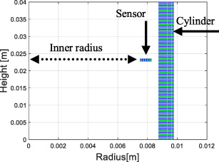
Geometry studied (half device).

Table 1

Geometry and physical parameters

Geometry and physical parameters	Sensor	Test-piece
Thickness [m]	0.75 ×10⁻³	Changing value
Height [m]	0.75 ×10⁻³	40 ×10⁻³
Inner radius [m]	7.5 ×10⁻³	8.75 ×10⁻³
Magnetic permeability [H/m]	4π ×10⁻⁷	4π ×10⁻⁷
Electric resistivity [Ω⋅m]	1/(5.59 ×10⁺⁷)	1/(37.7 ×10⁺⁶ )

Fig. 5.

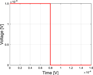
Source voltage waveform.

Fig. 6.

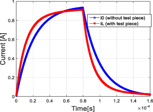
Input currents variation with time.

4.2. Results and discussions

4.2.1. Test-piece thickness variation

Firstly, we consider a 2D cylindrical and axisymmetric device with different cylinder thicknesses by imposing a constant value of the internal diameter. The coupled circuits model developed permits to get the results given in Fig. 7, representing the variation of the current Δi with time for different values of thickness.

Fig. 7.

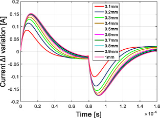
Current Δi (t) variation with thickness.

The previous results provided in Fig. 7 allows us to built the graphs representing the variation of the peak value of the current Δi (I_max) and the zero-crossing time (T₀) with the test-piece thickness variation (Figs 8 and 9). One can notice that these particular points (peak value, zero-crossing time) constitute important data for the assessment of the thickness of the test-piece. These results are compared to finite elements (FE) calculations and it show that the obtained results are very closed to those given by FE computation. Finally, for computational interest, the algebraic system is solved for 1600 time steps after 26 s, time step Δt = 10⁻⁷ [s] using a computer with 2.4 GHz of frequency and 16 GB RAM. In a future study a time computation comparison with FE method for specific cases (small air-gaps,...) will be considered.

Fig. 8.

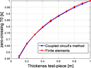
Zero-crossing T₀ results: Comparison between coupled circuits method and FE [10].

Fig. 9.

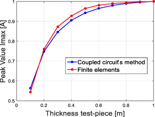
Peak value I_max results: Comparison between coupled circuits method and FE [10].

4.2.2. Variation of lift-off and electric conductivity

In the practice, it must have a distance between the sensor and the test-piece, to avoid rubbings. Besides, because of the variation of coating thickness, irregularity of the test-piece surface and of the vibrations during the movement of the sensor, the lift off remains hardly the same. This variation of the lift-off causes distortions in responses [2,11]. In theory the study of the variation of lift off could be simulated as a change of the sensor diameter or the one of the cylindrical test-piece. In our study the lift off variation is simulated as a test-piece internal diameter variation by imposing a constant value of the thickness of the cylinder.

Fig. 10.

Peak value I_max variation with lift off.

The Fig. 11 represents the variation of the current Δi with time for different values of the lift-off. In Fig. 10 we can note the decreases of the peak current with lift-off size when the latter is increasing. As noted the presence of the fixed point which remains unchanged with variation of the air-gap. In Fig. 12 the variation of the current Δi with time is plotted for different conductivities. We can notice that the maximum value is highly increasing when the electric conductivity increases. This result underline the high sensitivity of the signal with the variation of the conductivity.

Fig. 11.

Current Δi (t) variation with lift-off.

Fig. 12.

Current Δi (t) variation with electric conductivity.

5. Conclusion

The coupled circuits model in pulsed current study permit to characterize the geometry and physical parameters of the device such as the thickness, the lift-off and the electric conductivity. From the obtained results, some charts can be drawn in view of their exploitations in the conception of the tools of non destructive evaluations.

The coupled circuits model has the advantage of providing accurate results and adapts the processing of the change in topology systems without need of re-meshing solving domain. The precision of the results is the main interest of the method used. The results are considered consistent with those provided in the literature [3,10].

References

Tian

G.Y.

and Mandache

, Study of lift-off invariance for pulsed eddy-current signals, IEEE Transactions on Magnetics45 (2009), 184–191.

Tian

G.Y.

Adewale

and Simm

, Research on spectral response of pulsed eddy current and NDE applications, Sensors and Actuators A: Physical189 (2013), 313–320.

Singh

Bapat

H.M.

Singh

B.P.

Bandyopadhyay

Puri

R.K.

and Badodkar

D.N.

, Evaluation of aluminum plate using pulsed eddy current technique, J. Inst. Eng. India94 (2013), 89–93.

Wun

and Kang

, Assessment of wall thinning in insulated ferromagnetic pipes using the time-to-peak of differential pulsed eddy-current testing signals, NDT&E International51 (2012), 24–29.

Liu

Zh.

Ren

Sh.

Ren

Abidin

I.M.Z.

and Chen

Zh.

, Pulse-modulation eddy current evaluation of interlaminar corrosion in stratified conductors: Semi-analytical modeling and experiments, Sensors (Basel)22 (2022), 3458.

Bouali

Mohellebi

and Yousfi

, Coupled circuit method applied to the detection of defects in a conductive multilayer device, Przeglad Elektrotechniczny03 (2021), 106–112.

Augustyniak

and Usarek

, Finite element method applied in electromagnetic NDTE: A review, Journal of Nondestructive Evaluation35 (2016), 1–15.

Delage

and Ernst

, Prediction of the current distribution in an inductor with symmetry of revolution intended for heating by MF and HF induction, Revue Générale D’électricité (RGE)4 (1984), 225–230.

Bouzidi

Maouche

Feliachi

and Berthiau

, Pulsed eddy current non destructive evaluation Based on coupled electromagnetic quantities, The European Physical Journal: Applied Physics57 (2012), 1–9.

10.

Menana

, Contribution to the study of an eddy current sensor in pulse, DEA Report, University of Nantes, France, 2006.

11.

Shu

Songling

Wei

and Peng

, Improved immunity to lift-off effect in pulsed eddy current testing with two-stage differential probes, Russian Journal of Non-Destructive Testing44 (2008), 138–144.