Transient thermographic signal analysis for thinning detection in composite plate

Abstract

Infrared thermography is an imaging technique that can be used to inspect materials for flaws and various degradations in a non destructive way. In this work, we focused on the use of fast models to recover information about the material properties from experimental measurements recorded over time. Two different modelling approaches are compared to each other and to experimental data acquired on a composite plate. Then, the model based inverse problem consisting in estimating the plate properties is discussed.

Keywords

Infrared thermography composite material plate thinning

1. Introduction

Infrared thermograhy is a popular imaging technique for the non-destructive inspection of materials, as it allows to quickly inspect large areas of the piece under test and produces digital records. This makes it compatible with new trends in industry like industry 4.0, where manufacturing process optimization and traceability are key issues. Several variants of this techniques are currently used, as a passive measurement technique or with a heat source functioning transient or harmonic regime [1].

This paper focuses on the use of fast models for the characterization of material thermal properties from experimental measurements obtained using an active source in transient regime. The first two sections present briefly these approaches, which are the quadrupole method [2], solving the heat equation in frequency domain, and the Finite Integration Technique (FIT) [3,4], solving it in time domain. The implementations of these approaches are 1D and 2D, respectively, which is sufficient for simple cases and yields high computational efficiency.

The third section describes the experimental procedure. The piece inspected is a reference block made of composite material and the heat source is a set of lamps driven with a step excitation signal. Finally, the fourth section discusses the model-based characterization of the piece thermal properties. It focuses on the inverse problem itself rather than a specific inversion method, as the models evaluation is not costly.

2. Simulation of the inspection procedure

Simulation of the thermal inspection of the piece can be decomposed in three steps. The first one is the modelling of the heat source, which is a set of halogen lamps in our case. Considering the experimental setup used in this work (see Fig. 1), a description of the source as a uniform energy distribution at the top of the piece is used, thus it is only defined by an amplitude term and a time signal.

The second step is the solution of the heat equation for the calculation of the temperature distribution in the piece over time. Two different approaches, presented hereafter, have been used to do so: the thermal quadrupoles and the Finite Integration Technique.

Finally the last step consists in the modelling of the thermal camera response to a particular temperature distribution at the observed surface of the piece. As the temperature variation observed is small (typically less than 10 °C) and the measurement is carried out in well controlled laboratory conditions, a linear response of the camera is assumed and, as it was not experimentally characterized, a calibration in amplitude is used to compare simulation results and experimental data.

Fig. 1.

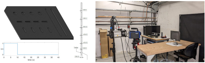
Experimental setup and characteristics of the mock-up used. The excitation signal is a step function.

2.1. Presentation of the thermal quadrupole formalism

This formalism allows, in its 1D version presented here, to address the case of an infinite planar stratified medium submitted to a spatially homogeneous excitation and to calculate the temperature distribution T (z, t) at its upper and lower surfaces. This quantity depends on the depth z and time t, as shown in Fig. 2. Each layer i of the stratified medium is defined by its thickness e_i and its material properties: thermal conductivity k_i, volumetric mass density 𝜚_i and specific heat capacity c_i.

The application of the Laplace transform to the heat equation and the definition of the heat flux 𝜙 leads to the set of Eqs (1) for the equivalent variables 𝜃 and 𝜓, depending each on the depth z and the Laplace variable p.

Fig. 2.

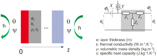
Illustration of the Quadrupoles formalism applied to a 1D stratified medium with convection losses.

This set of equations, expressed in a matrix form in Eqs (2) and (3) for single and multi-layer cases, respectively, shows that the evolution of temperature across the medium can be described in Laplace domain through a succession of quadrupole operators, characterizing each a given layer of the structure. This description is very similar to the one used to model electrical circuits, as illustrated in Fig. 2. $\begin{eqnarray}\displaystyle \text{} & \text{} & \displaystyle {\displaystyle \frac{d^{2}T}{dz^{2}}}={\displaystyle \frac{{\varrho}c}{k}}{\dot{T}}\rightarrow {\displaystyle \frac{d^{2}{\theta}}{dz^{2}}}={\displaystyle \frac{{\varrho}c}{k}}p{\theta},\qquad {\phi}=-k{\displaystyle \frac{dT}{dz}}\rightarrow {\psi}=-k{\displaystyle \frac{d{\theta}}{dz}}\end{eqnarray}$ (1) $\begin{eqnarray}\displaystyle \text{} & \text{} & \displaystyle {\displaystyle \frac{d}{dz}}\left[\begin{array}{@{}c@{}}{\theta}\\ {\psi}\end{array}\right]=\left[\begin{array}{@{}cc@{}}0 & -1/k\\ -{\varrho}∼c∼p & 0\end{array}\right]\left[\begin{array}{@{}c@{}}{\theta}\\ {\psi}\end{array}\right]\end{eqnarray}$ (2) $\begin{eqnarray}\displaystyle \text{} & \text{} & \displaystyle \left[\begin{array}{@{}c@{}}{\theta}(z=0)\\ {\psi}(z=0)\end{array}\right]=\left[\begin{array}{@{}cc@{}}A_{1} & B_{1}\\ C_{1} & D_{1}\end{array}\right]\cdots \left[\begin{array}{@{}cc@{}}A_{n} & B_{n}\\ C_{n} & D_{n}\end{array}\right]\left[\begin{array}{@{}c@{}}{\theta}\left(z=\displaystyle \mathop{\sum }_{i}e_{i}\right)\\[12.0pt] {\psi}\left(z=\displaystyle \mathop{\sum }_{i}e_{i}\right)\end{array}\right].\end{eqnarray}$ (3)

In this formalism, boundary conditions applied to the upper and lower surfaces, as well as convection losses, defined as an additional term 𝜓_c = ±h. 𝜃 to the heat flux, are also described using quadrupoles. The convection parameter h depends on the environment and is often hard to characterize. However, in the case of a pulse excitation it can be fitted from measurements carried out at longer times, where convection predominates over conduction. $\begin{eqnarray}\displaystyle T(z,t)={\displaystyle \frac{ln(2)}{t}}\mathop{\sum }_{m=1}^{N}V_{m}∼.∼{\theta}\left(z,m{\displaystyle \frac{ln(2)}{t}}\right). & & \displaystyle\end{eqnarray}$ (4)

Once the solution 𝜃(z, t) has been calculated, one has to invert the Laplace transform to get the solution T (z, t) in time domain. Among the various ways to do so, we selected the numerical Stehfest method [5] defined in Eq. (4). The order of the method N = 20, meaning that each value in time is computed from 20 values in Laplace domain, was chosen to get a good compromise between accuracy and time efficiency.

2.2. Presentation of the finite integration technique

The 1D thermal quadripole approach is not well adapted for treating problems where lateral diffusion effects are significant, as in the case of interaction between neighbouring defects [6], or when arbitrary excitation signals need to be considered. In these cases, one must resort to a more versatile numerical technique such as the FIT.

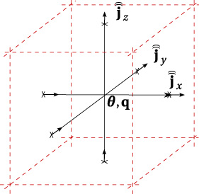
According to the FIT approach, the energy conservation equation and Fourier’s law are discretised using a couple of staggered orthogonal grids, with the temperature field 𝜽 being allocated to the nodes of the primary grid and the heat flux field $\stackrel{\frown}{\overset{\frown}{\mathbf{j}}}$ being integrated at the facets of the dual grid as shown in Fig. 3.

Fig. 3.

Allocation of the state variables on the FIT dual grid system.

Integrating the energy conservation equation in the volume of all primary grid cells and and Fourier’s law across the flux tubes defined between the primary nodes, we end up with the FIT matrix equations, which stand for the discrete version of two laws: $\begin{eqnarray} \displaystyle \mathbf{M}_{C}\dot{\boldsymbol{\boldsymbol{\it\theta}}} & = & \displaystyle \dot{\mathbf{q}}-\widetilde{\mathbf{S}}\stackrel{\frown}{\overset{\frown}{\mathbf{j}}} \end{eqnarray}$ (5) $\begin{eqnarray} \displaystyle \mathbf{M}_{{\kappa}}^{-1}\stackrel{\frown}{\overset{\frown}{\mathbf{j}}} & = & \displaystyle -\mathbf{G}\boldsymbol{\boldsymbol{\it\theta}} \end{eqnarray}$ (6) where G and $\widetilde{\mathbf{S}}$ are the discrete grad and div topological operators applying to the vector spaces spanned by the primary and dual grid, respectively, and M_C, M_𝜅 are diagonal matrices comprising the heat capacity of the primary grid cells and the averaged thermal conductivity at the dual cell facets. Finally, q stand for the integrated heat sources across the primary cells. For a detailed definition of the variables appearing in (5), (6) the reader is referred to [4].

The contribution of the convection and radiation mechanisms can be taken into account by including an additional loss term at the right-hand-side of the energy conservation equation (5). For small temperature changes during the heating process, the combined radiation-convection losses can be approximated by the linear term M_h(𝜽 − 𝜽₀), where 𝜽₀ stands for the ambient (initial) temperature and M_h a diagonal matrix assembling the equivalent loss coefficient at the nodes of the free specimen surfaces [1 ].

Combination of (5) with (6) yields the state equation $\begin{eqnarray}\displaystyle (\widetilde{\mathbf{S}}\mathbf{M}_{{\kappa}}\mathbf{G}+\mathbf{M}_{h})\boldsymbol{\boldsymbol{\it\theta}}-\mathbf{M}_{C}\dot{\boldsymbol{\boldsymbol{\it\theta}}}=-\dot{\mathbf{q}}+\mathbf{M}_{h}\boldsymbol{\boldsymbol{\it\theta}}_{0}. & & \displaystyle\end{eqnarray}$ (7) Equation (7) must be integrated in time in order to obtain the temperature distribution during the considered time window. Since the heat equation is a diffusion equation, this integration has to be carried out using implicit time-stepping schemes as in the case of the eddy currents [7]. The advantage solving the heat equation directly in the time domain lies in the ability of treating arbitrary waveforms for the source term q, in contrast to the use of the Laplace transform, whose inversion can be numerically cumbersome in cases of non-monotonic excitations.

3. Experimental procedure and comparison results

Experimental acquisitions have been recorded in laboratory conditions on a reference planar carbon fiber reinforced polymer (CFRP) specimen containing large flaws with different shapes, using a FLIR SC 7000 thermal camera, as illustrated in Fig. 1. Its material properties are given in Table 1. Two lamps with a power of 2 kW each were used as homogeneous heat sources and were driven with a rectangular pulse signal (10 s of excitation for a total duration of 40 s). Experimental time signals are extracted from the complete thermogram for areas with remaining thickness of 1 mm, 2 mm, 3 mm and 9 mm, respectively, as illustrated in Fig. 4.

One can see on this curves the effect of convection as a linear decrease of temperature with respect to time for t ≥ 20 s, which is more important for a small thickness than for a large one, as it can be expected. As the convection phenomenon dominates after the transient regime consecutive to the thermal excitation, the values of this slope for different thicknesses constitutes a relevant set of indicators for the estimation of the convection coefficient h. Three different areas of the curves can thus be identified: the heating part for t ≤ 10 s, a rapid temperature decrease for 10 s ≤ t ≤ 20 s, and an asymptotic regime where convection dominates for t ≥ 20 s.

Table 1
Estimation results of the material thermal conductivity k, specific heat 𝜚. c and diffusivity a using the 1D quadrupole model

k (W.m⁻¹.K⁻¹) 𝜚. c (J.m⁻³ .K⁻¹ ) a (m² .s⁻¹ )

Reference values 0.63 1.58 10⁶ 4.0 10⁻⁷

Estimated values 0.65 1.8 10⁶ 3.61 10⁻⁷

	k (W.m⁻¹.K⁻¹)	𝜚. c (J.m⁻³ .K⁻¹ )	a (m² .s⁻¹ )
Reference values	0.63	1.58 10⁶	4.0 10⁻⁷
Estimated values	0.65	1.8 10⁶	3.61 10⁻⁷

Fig. 4.

Experimental data used for the comparison with simulation results: top view and time signals corresponding to several areas of the mock-up.

Fig. 5.

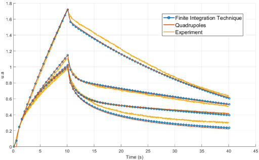
Comparison of simulation results with respect to experimental data.

Fig. 6.

Visualization of the cost function with respect to 𝜚. c, k, h and reduced cost function obtained with a fixed value of the h coefficient.

4. Model based characterization of material properties

In order to check the relevance of both modelling approaches, simulation results obtained with reference values for material properties k and 𝜚. c (see Table 1) are first compared to experimental data. On Fig. 5, a calibration coefficient is applied to simulation results so that maximal amplitudes of the highest curves (corresponding to the smallest thickness of 1 mm) match. As mentioned before, the convection parameter h is chosen empirically to get the best agreement. Comparison results are quite satisfactory, as simulated curves reproduce accurately, and for all thicknesses, the shape and amplitudes of the experimental curves in the three areas (heating time, rapid decay, asymptotic regime). This qualifies both models for the estimation of material parameters.

In a practical situation, one has to add h to k and 𝜚. c as unknown parameters to estimate. If we consider a simple cost function, consisting in the mean square error between experimental and simulated time signal, we can visualize in Fig. 6 (left plot) the isosurfaces corresponding to the lowest values of this indicator with respect to our three unknowns. This figure shows clearly that the estimation for all parameters at once is an ill-posed problem, as the isosurfaces have a pencil shape indicating that many combinations lead to similar values. However, if we determine the convection parameter h first from the slopes of the curves in the asymptotic regime, the estimation problem becomes quite well posed, as there is no doubt where the global minimum of the cost function is located. From a quantitative point of view (see Table 1, where corresponding values of diffusivity $a=\frac{k}{{\varrho}.c}$ are also given for reference), the estimation of these two parameters using this simple brute force approach is satisfactory in this case. In more complex situations, the modelling approach required would be more complex and the associated computational time would not permit to carry out so many evaluations. The use of more sophisticated estimation approaches [6] would then be justified.

5. Conclusions and perspectives

In this work, two different modelling approaches were used to simulate a thermographic inspection, in view of estimating material thermal properties. The first approach is a 1D implementation of the thermal quadrupoles method, solving the heat equation in the Laplace domain, and the second one is a 2D implementation of the Finite Integration Technique, based on a grid discretization in space and a time stepping method in time. Both methods reproduce accurately experimental data obtained in laboratory conditions with a homogeneous source and a step excitation signal. Then the model based estimation problem of material thermal conductivity k and specific heat 𝜚. c is discussed. In practical situations, losses due to convection have to be also characterized, which adds a parameter h to the unknowns. However, in order to avoid facing an ill-posed inverse problem, it is a good strategy, for this type of excitation, to estimate the convection parameter h first, using for instance the temperature decay rate at longer times. Then, the material parameters can be estimated accurately.

References

Maldague

X.P.V.

and Moore

P.O.

, Nondestructive Testing Handbook: Infrared and Thermal Testing, Vol. 3, The American Society for Nondestructive Testing, 2001.

Maillet

André

Batsale

J.C.

Degiovanni

and Moyne

, Thermal Quadrupoles: Soving the Heat Equation through Integral Transforms, First edn, John Willey & Sons, Inc., 2000.

Clemens

Gjonaj

Pinder

and Weiland

, Self-consistent simulations of transient heating effects in electrical devices using the finite integration technique, IEEE Transactions on Magnetics37(5) (2001), 3375–3379, doi:10.1109/20.952617.

Skarlatos

, Near-field scattering solutions using mixed bases with application to electromagnetic and thermographic ispection of technical materials, Habilitation à diriger des recherches, Université Paris-Saclay, January 2023. https://hal.science/tel-04052729.

Stehfest

, Algorithm 368. Numerical inversion of the Laplace transforms, Communications of the ACM 13(1) (1970), 47–49.

Ratsakou

Skarlatos

Reboud

and Lesselier

, Shape reconstruction of delamination defects using thermographic infrared signals based on an enhanced Canny approach, Infrared Physics and Technology111 (2020), 103527, doi:10.1016/j.infrared.2020.103527, https://centralesupelec.hal.science/hal-02617537.

Skarlatos

and Reboud

, A hybrid spectral-spatial formulation for the calculation of the transient eddy-current response, International Journal of Applied Electromagnetics and Mechanics (2023), Submitted for publication.

Transient thermographic signal analysis for thinning detection in composite plate

Abstract

Keywords

1. Introduction

2. Simulation of the inspection procedure

Table 1 Estimation results of the material thermal conductivity k, specific heat 𝜚. c and diffusivity a using the 1D quadrupole model k (W.m−1.K−1) 𝜚. c (J.m−3 .K−1 ) a (m2 .s−1 ) Reference values 0.63 1.58 106 4.0 10−7 Estimated values 0.65 1.8 106 3.61 10−7

5. Conclusions and perspectives

References

Table 1
Estimation results of the material thermal conductivity k, specific heat 𝜚. c and diffusivity a using the 1D quadrupole model

k (W.m⁻¹.K⁻¹) 𝜚. c (J.m⁻³ .K⁻¹ ) a (m² .s⁻¹ )

Reference values 0.63 1.58 10⁶ 4.0 10⁻⁷

Estimated values 0.65 1.8 10⁶ 3.61 10⁻⁷