Application of implicit symplectic difference scheme in calculating propagation trajectory of wave in non-magnetized plasma

Abstract

Ray tracing method is an important tool of studying wave propagation in plasma. The ray tracing equations are Hamiltonian and usually calculated by traditional Runge-Kutta-Fehlberg method. Symplectic geometric structure of Hamiltonian system is not considered in Runge-Kutta-Fehlberg method. In order to preserve the symplectic geometric structure of Hamiltonian system, symplectic geometric algorithm is used to solve ray tracing equations. In a calculation example, the propagation trajectories of waves in non-magnetized plasmas are calculated by using the symplectic geometric algorithm, and the results are compared with those obtained by Runge-Kutta-Fehlberg algorithm. The results show that the symplectic geometric algorithm has a unique advantage in maintaining the propagation trajectory and dispersion function value.

Keywords

Symplectic geometric algorithm ray tracing plasmaPACS: 52.35.-g 52.65.-y

1. Introduction

Feng and his coworkers created the symplectic geometric algorithms for Hamiltonian systems, according to geometric structure of Hamiltonian systems [1, 2, 3, 4, 5, 6, 7]. Compared to the traditional algorithm, the symplectic geometric algorithm can keep the geometric structure unchanged. Theoretical and numerical analysis showed that the symplectic geometric algorithm is an effective method to simulate the long-term behavior of Hamiltonian systems [8, 9].

Ray tracing is a geometric optics approximation [10], in which the parameters of the medium are assumed to change little in a wavelength. In one dimension case it means that $(\frac{d}{dx}\ln(A))^{-1}\gg\lambda$ , A is some parameter of the medium. The ray tracing technique is based on the WKB approximation, which holds as long as the amplitude is slowly varying.The field strength of the wave can be seen as consisting of two parts: the first part is slowly changing amplitude,and the other part is fast changing phase. This method is widely used to study the propagation of radio waves in plasma [11, 12, 13, 14, 15, 16, 17, 18]. When the waves propagating in the plasma are slightly disturbed and the plasma waves are linearly absorbed or without absorption, the ray trajectory equations have a Hamiltonian form. The usual method for solving the Hamiltonian ray trajectory equation is the Runge-Kutta-Fehlberg method. Hereinafter referred to as RKF method. The traditional RKF method does not take into account the symplectic geometric structure of the Hamiltonian system, and the difference scheme does not guarantee that the transformation between two steps is symplectic. In this paper, the general form of the implicit symplectic difference scheme for ray tracing equation is derived, and the advantage of symplectic geometric algorithm over a traditional algorithm is shown by a calculation example.

2. Symplectic difference schemes of ray tracing equation in non-magnetized plasma

Let D be the wave’s dispersion function, D is 0 at any point on the ray trajectory. D can be written as D ( $\overrightarrow{k}$ , $w$ , $\overrightarrow{r}$ , $t$ ), where $\overrightarrow{k}$ is the wave vector, $\overrightarrow{r}$ represents spatial position on the ray trajectory, $w$ is the wave frequency, $t$ is propagation time. The ray tracing equations can be written as:

$\displaystyle\frac{d\vec{r}}{d\tau}=-\frac{\partial D}{\partial\vec{k}}$ (1) $\displaystyle\frac{d\vec{k}}{d\tau}=\frac{\partial D}{\partial\vec{r}}$ (2) $\displaystyle\frac{dt}{d\tau}=\frac{\partial D}{\partial w}$ (3)

Equations (1) and (2) are Hamiltonian form, the dispersion function D is Hamiltonian. In non-magnetized plasma, the dispersion relationship of transverse wave is

$\displaystyle D=w^{2}-c^{2}k^{2}-\sum\limits_{\alpha}{w_{p\alpha}^{2}}=0$ (4) $\displaystyle w_{p\alpha}^{2}=\frac{n_{\alpha}q_{\alpha}^{2}}{\varepsilon_{0}m% _{\alpha}}$ (5)

$\alpha$ means particle species in plasma, usually including electrons and more than one species of positive ion. $w_{p\alpha}$ denotes the oscillation frequency of $\alpha$ species particles, it is called plasma frequency. $n$ is the particle density, $m$ is the particle mass, $q$ is the particle charge, $\varepsilon_{0}$ is The dielectric constant in vacuum. For high frequency waves, only the response of electrons to waves is considered. The response of ions to waves is not considered. So the dispersion relation of the transverse wave can be simplified as

$\displaystyle D=w^{2}-c^{2}k^{2}-w_{pe}^{2}=0$ (6) $\displaystyle\frac{dt}{d\tau}=2w$ (7)

By the above Eqs (1) and (2) can be written as

$\displaystyle\frac{d\vec{r}}{dt}=-\frac{1}{2w}\frac{\partial D}{\partial\vec{k}}$ (8) $\displaystyle\frac{d\vec{k}}{dt}=\frac{1}{2w}\frac{\partial D}{\partial\vec{r}}$ (9)

In the propagation without considering the nonlinear effect, the wave frequency $w$ remains a constant. Then the Hamiltonian in Eqs (8) and (9) can be written as

$\displaystyle H=\frac{1}{2w}\left(-c^{2}k^{2}-\frac{q_{e}^{2}n_{e}}{% \varepsilon_{0}m_{e}}\right)$ (10)

Equations (8) and (9) can be expressed as

$\displaystyle\frac{d\vec{r}}{dt}=-\frac{\partial H}{\partial\vec{k}}$ (11) $\displaystyle\frac{d\vec{k}}{dt}=\frac{\partial H}{\partial\vec{r}}$ (12)

Let $p=(x\ \ y\ \ z\ \ {k_{x}}\ \ {k_{y}}\ \ {k_{z}})^{T}$ Eqs (11) and (12) can be written as

$\displaystyle\frac{dp}{dt}=J^{-1}\frac{\partial H}{\partial p}$ (13)

$J^{-1}$ is the inverse of the symplectic matrix $J$ .

$\displaystyle J=\left({{\begin{array}[]{*{20}c}0\hfill&I\hfill\\ {-I}\hfill&0\hfill\\ \end{array}}}\right)$ (14)

$I$ is a 3 $\times$ 3 identity matrix.

According to symplectic geometric algorithms, the implicit symplectic difference scheme of the above equations can be constructed [19]. Such as the fourth order implicit symplectic difference scheme is

$\displaystyle p^{n+1}=p^{n}+dtJ^{-1}\nabla H\left|{{}_{p=\frac{p^{n{+1}}+p^{n}% }{2}}}\right.-\frac{dt^{3}}{24}J^{-1}\nabla[(\nabla H)^{T}JH_{pp}J\nabla H]% \left|{{}_{p=\frac{p^{n{+1}}+p^{n}}{2}}}\right.$ (15) $\displaystyle\nabla H=\left({\begin{array}[]{*{20}c}{\frac{\partial H}{% \partial x}}\hfill&{\frac{\partial H}{\partial y}}\hfill&{\frac{\partial H}{% \partial z}}\hfill&{\frac{\partial H}{\partial k_{x}}}\hfill&{\frac{\partial H% }{\partial k_{y}}}\hfill&{\frac{\partial H}{\partial k_{z}}}\hfill\\ \end{array}}\right)^{T}$ (16) $\displaystyle H_{pp}=\left({{\begin{array}[]{*{20}c}{\frac{\partial^{2}H}{% \partial x^{2}}}\hfill&{\frac{\partial^{2}H}{\partial x\partial y}}\hfill&{% \frac{\partial^{2}H}{\partial x\partial z}}\hfill&{\frac{\partial^{2}H}{% \partial x\partial k_{x}}}\hfill&{\frac{\partial^{2}H}{\partial x\partial k_{y% }}}\hfill&{\frac{\partial^{2}H}{\partial x\partial k_{z}}}\hfill\\ {\frac{\partial^{2}H}{\partial y\partial x}}\hfill&{\frac{\partial^{2}H}{% \partial y^{2}}}\hfill&{\frac{\partial^{2}H}{\partial y\partial z}}\hfill&{% \frac{\partial^{2}H}{\partial y\partial k_{x}}}\hfill&{\frac{\partial^{2}H}{% \partial y\partial k_{y}}}\hfill&{\frac{\partial^{2}H}{\partial y\partial k_{z% }}}\hfill\\ {\frac{\partial^{2}H}{\partial z\partial x}}\hfill&{\frac{\partial^{2}H}{% \partial z\partial y}}\hfill&{\frac{\partial^{2}H}{\partial z^{2}}}\hfill&{% \frac{\partial^{2}H}{\partial z\partial k_{x}}}\hfill&{\frac{\partial^{2}H}{% \partial z\partial k_{y}}}\hfill&{\frac{\partial^{2}H}{\partial z\partial k_{z% }}}\hfill\\ {\frac{\partial^{2}H}{\partial k_{x}\partial x}}\hfill&{\frac{\partial^{2}H}{% \partial k_{x}\partial y}}\hfill&{\frac{\partial^{2}H}{\partial k_{x}\partial z% }}\hfill&{\frac{\partial^{2}H}{\partial k_{x}^{2}}}\hfill&{\frac{\partial^{2}H% }{\partial k_{x}\partial k_{y}}}\hfill&{\frac{\partial^{2}H}{\partial k_{x}% \partial k_{z}}}\hfill\\ {\frac{\partial^{2}H}{\partial k_{y}\partial x}}\hfill&{\frac{\partial^{2}H}{% \partial k_{y}\partial y}}\hfill&{\frac{\partial^{2}H}{\partial k_{y}\partial z% }}\hfill&{\frac{\partial^{2}H}{\partial k_{y}\partial k_{x}}}\hfill&{\frac{% \partial^{2}H}{\partial k_{y}^{2}}}\hfill&{\frac{\partial^{2}H}{\partial k_{y}% \partial k_{z}}}\hfill\\ {\frac{\partial^{2}H}{\partial k_{z}\partial x}}\hfill&{\frac{\partial{}^{2}H}% {\partial k_{z}\partial y}}\hfill&{\frac{\partial^{2}H}{\partial k_{z}\partial z% }}\hfill&{\frac{\partial^{2}H}{\partial k_{z}\partial k_{x}}}\hfill&{\frac{% \partial^{2}H}{\partial k_{z}\partial k_{y}}}\hfill&{\frac{\partial^{2}H}{% \partial k_{z}^{2}}}\hfill\\ \end{array}}}\right)$ (17)

Arbitrary even order accuracy can be obtained by using the symplectic geometrical algorithm. There is no even power of time step in the implicit difference scheme. This greatly simplifies the calculation and increases the speed of operation. The generating function is odd about time step [20], so there is no even term of time step in the expansion of the generating function.

Figure 1.

Position deviation changes over time.

3. Calculation example

In the two-dimensional case, the electron density profile of non-magnetized plasma is assumed to be

$\displaystyle n(x,y)=n_{0}\left[1+\left(\frac{x^{2}+y^{2}}{R^{2}}\right)^{1/2}\right]$ (18)

where $n_{0}$ and $R$ are constants. Then the transverse wave dispersion function is

$\displaystyle D(x,y,k_{x},k_{y})=-c^{2}(k_{x}^{2}+k_{y}^{2})+w^{2}-w_{p}^{2}(x% ,y)$ (19) $\displaystyle w_{p}^{2}(x,y)=w_{p0}^{2}\left[1+\left(\frac{x^{2}+y^{2}}{R^{2}}% \right)^{1/2}\right]$ (20) $\displaystyle w_{p0}^{2}=\frac{n_{0}q_{e}^{2}}{\varepsilon_{0}m_{e}}$ (21) $\displaystyle H=\frac{1}{2w}\left\{-c^{2}k^{2}-\frac{q_{e}^{2}}{\varepsilon_{0% }m_{e}^{2}}\left[1+\left(\frac{x^{2}+y^{2}}{R^{2}}\right)^{{1/2}}\right]\right\}$ (22)

Related physical quantities are normalized, $x\sim R$ , $y\sim R$ , $k_{x}\sim 1/R$ , $k_{y}\sim 1/R$ , $t\sim 1/w_{p0}$ , $w\sim w_{p0}$ , $c\sim Rw_{p0}$ . Thus the normalized differential equations are written as

$\displaystyle\frac{d\tilde{x}}{d\tilde{t}}=\frac{\tilde{c}^{2}}{\tilde{w}}% \tilde{k}_{x}$ (23) $\displaystyle\frac{d\tilde{y}}{d\tilde{t}}=\frac{\tilde{c}^{2}}{\tilde{w}}% \tilde{k}_{y}$ (24) $\displaystyle\frac{d\tilde{k}_{x}}{d\tilde{t}}=-\frac{\tilde{x}}{2\tilde{w}% \sqrt{\tilde{x}^{2}+\tilde{y}^{2}}}$ (25) $\displaystyle\frac{d\tilde{k}_{y}}{d\tilde{t}}=-\frac{\tilde{y}}{2\tilde{w}% \sqrt{\tilde{x}^{2}+\tilde{y}^{2}}}$ (26) $\displaystyle\frac{d\tilde{p}}{d\tilde{t}}=J^{-1}\nabla\tilde{H}$ (27) $\displaystyle\tilde{p}=\left({{\begin{array}[]{*{20}c}\tilde{x}\hfill&\tilde{y% }\hfill&{\tilde{k}_{x}}\hfill&{\tilde{k}_{y}}\hfill\\ \end{array}}}\right)^{T}$ (28) $\displaystyle\tilde{H}=\frac{1}{2\tilde{w}}[-\tilde{c}^{2}(\tilde{k}_{x}^{2}+% \tilde{k}_{y}^{2})-(1+\sqrt{\tilde{x}^{2}+\tilde{y}^{2}})]$ (29)

The initial conditions are

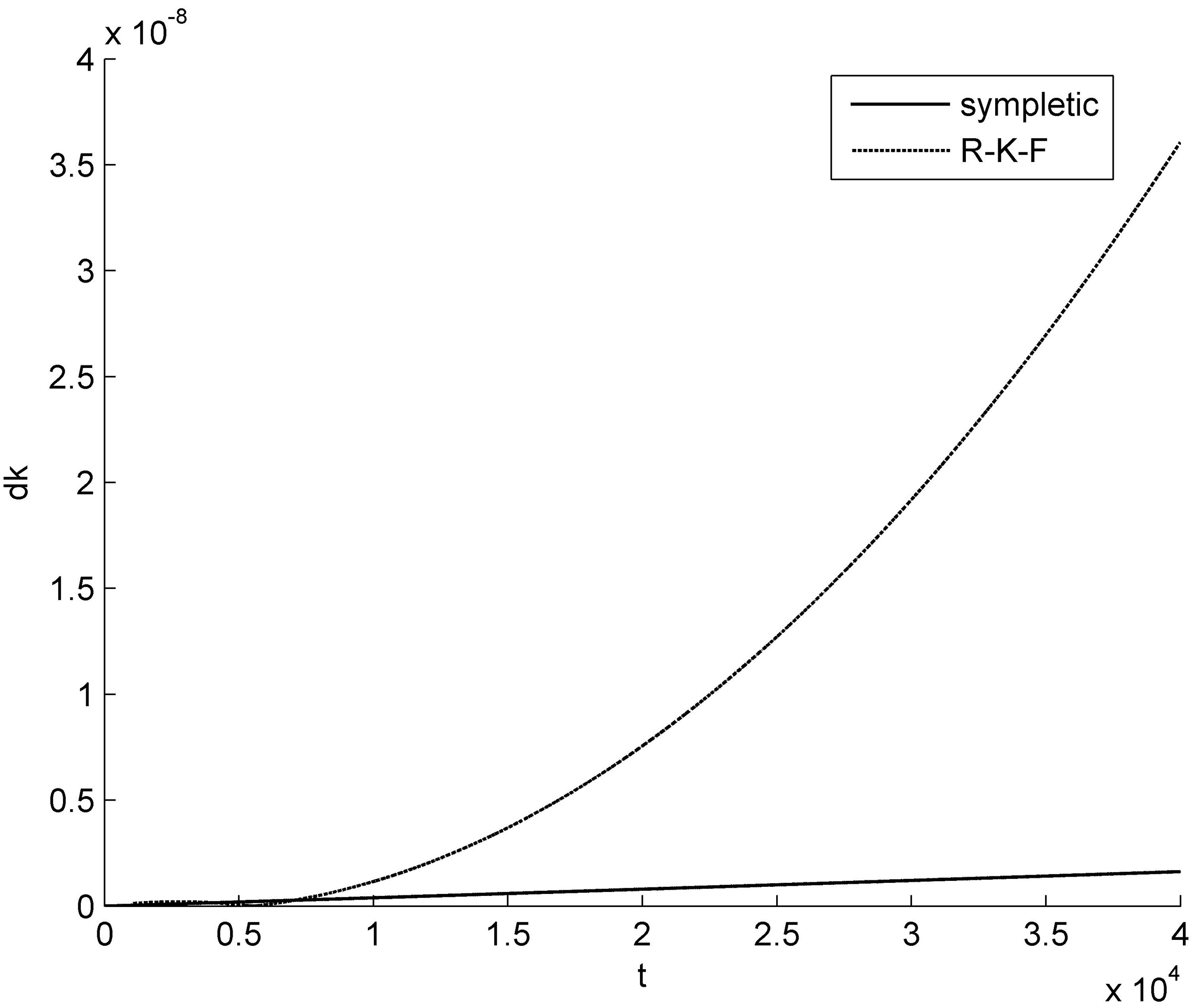
$\tilde{x}=2(\tilde{w}^{2}-1)/3\tilde{y}=0\tilde{k}_{x}=0\tilde{w}=3d\tilde{t}=% 0.1_{.}$

Figure 2.

Wave vector deviation changes over time.

Figure 3.

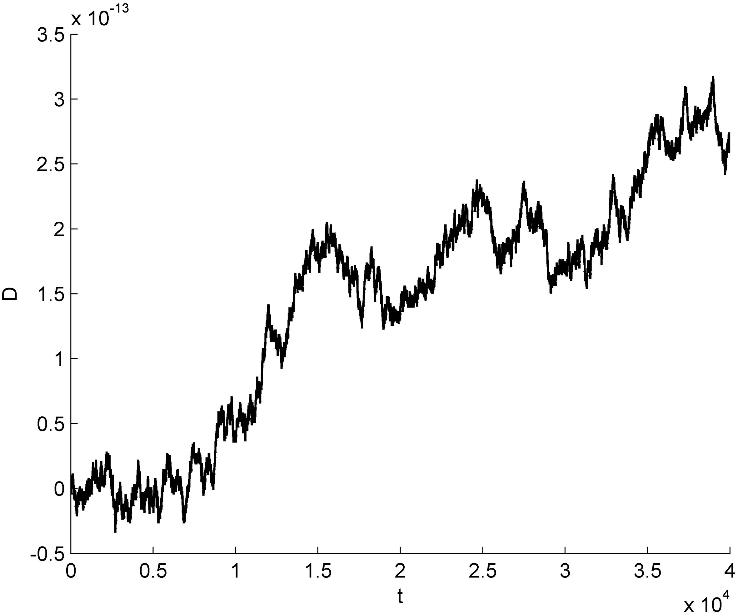
The dispersion function value changes over time in symplectic geometric method.

Figure 4.

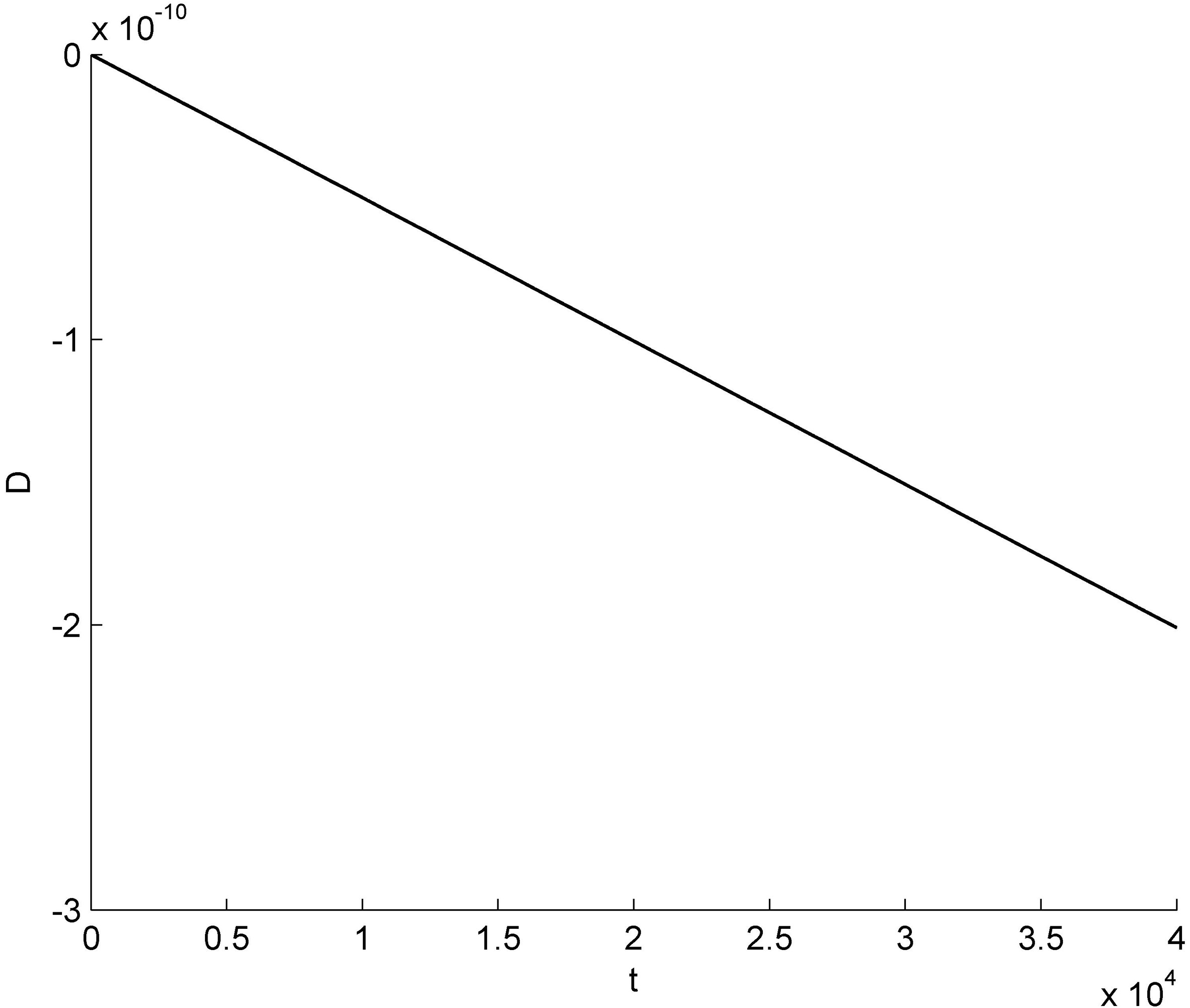
The dispersion function value changes over time in RKF method.

From the analytical solution, we can see that the propagation path of this beam is a circle. Figure 1 shows the position deviations between the analytical solution, and the propagation trajectory obtained by using the fourth-order symplectic difference scheme and the RKF scheme. The position deviation is defined as $dr=\sqrt{(\tilde{x}_{nc}-\tilde{x}_{ana})^{2}+(\tilde{y}_{nc}-\tilde{y}_{ana})% ^{2}}$ where the subscript ncrepresents the results obtained by using the fourth-order symplectic difference scheme and the RKF scheme. The subscript ana represents the analytical solution. From Fig. 1 it can be seen that the trajectory deviation calculated by the symplectic difference scheme increases linearly with time, and the trajectory deviation calculated by the RKF scheme increases non-linearly with time. Figure 2 shows the wave vector deviation of the analytical solution and the wave vector obtained by the fourth-order symplectic difference scheme and the RKF scheme. The wave vector deviation is defined as $dk=\sqrt{(\tilde{k}_{x,nc}-\tilde{k}_{x,ana})^{2}+(\tilde{k}_{y,nc}-\tilde{k}_% {y,ana})^{2}}$ . Figure 2 shows that the wave vector deviation of the results calculated by the symplectic difference scheme increases linearly with time, and the deviation of the results calculated by the RKF scheme increases with time. As time goes on, the advantages of the symplectic difference scheme are becoming more apparent. Figures 3 and 4 show the change of the dispersion function values calculated bysymplectic difference scheme and the RKF scheme respectively over time. In the wave propagation, the dispersion function value is a constant for zero. From these two graphs, it can be seen that the accuracy of the dispersion function value in the symplectic difference scheme is higher 2–3 orders than that in the RKF scheme.In the symplectic difference scheme, the dispersion function value oscillates over time in a small range, ensuring high accuracy of the dispersion function values over a long period of time. In the RKF scheme, the absolute value of dispersion function increases linearly with time, and the dispersion function value cannot be maintained over a long period of time.

4. Conclusion

By comparing the symplectic geometric algorithm with the traditional numerical algorithm, we can see the advantage of the symplectic geometric algorithm in maintaining the dispersion function value. The symplectic geometric algorithm can maintain a relatively stable dispersion function value. The propagation trajectory calculated by symplectic geometric algorithm has a high degree of credibility. In this paper, the case of non-magnetized plasma is considered. The next step is to consider the application of symplectic geometric algorithm in complex magnetic field.

References

Feng

, Journal of Computational Mathematics 4(3) (1986), 279–289.

Feng

and Qing

M.Z.

, Hamiltonian algorithms for Hamiltonian systems and a comparative numerical study, Computer Physics Communications 65 (1991), 173–187.

Feng

, Formal power series and numerical algorithms for dynamical systems, Series on Applied Mathematics 1 (1991), 28–35.

Feng

and Wang

D.L.

, Symplectic difference schemes for Hamiltonian systems in general symplectic structure, Journal of Computational Mathematics 9(1) (1991), 86–96.

Feng

and Shang

, Volume-preserving algorithms for source-free dynamical systems, Numerische Mathematik 71(4) (1995), 451–463.

Feng

, The calculus of generating functions and the formal energy for Hamiltonian algorithms, Journal of Computational Mathematics 16(6) (1998), 481–498.

Feng

, The step-transition operators for multi-step methods of ODE’s, Journal of Computational Mathematics 16(3) (1998), 193–202.

Liu

S.X.

et al., The application of symplectic geometric algorithm in a special Chaplygin system, Acta Physica Sinica 60(3) (2011), 034501 (in Chinese).

Liu

S.X.

and Ding

P.Z.

, New progress of structure-preserving computation for quantum system, Progress in Physics 24(1) (2004), 47–89 (in Chinese).

10.

Bernstein

I.B.

, Geometric optics in space- and time- varying plasmas, Physics of Fluids 18(3) (1975), 320–324.

11.

Smirnov

A.P.

and Harvey

R.W.

, Calculations of the current drive in DIII-D with the GENRAY ray tracing code, Bulletin of the American Physical Society 40 (1995), 1837–1842.

12.

Yang

et al., Modelling of the EAST lower-hybrid current drive experiment using GENRAY/CQL3D and TORLH/CQL3D, Plasma Physics and Controlled Fusion 56(12) (2014), 125003.

13.

Esterkin

A.R.

and Piliya

A.D.

, Fast ray tracing code for LHCD simulations, Nuclear Fusion 36(11) (1996), 1501–1512.

14.

McVey

B.D.

, A ray-tracing analysis of fast-wave heating of tokamaks, Nuclear Fusion 19(4) (1979), 461–468.

15.

Baranov

Y.F.

and Fedorov

V.I.

, Lower-hybrid wave propagation in tokamaks, Nuclear Fusion 20(9) (1980), 1111–1118.

16.

Brambilla

M.A.

et al., Eikonal description of HF waves in toroidal plasmas, Plasma Physics 24(10) (1982), 1187–1218.

17.

Bonoli

, Linear theory of lower hybrid heating, IEEE Transactions on Plasma Science 12(2) (1984), 95–107.

18.

Casolari

and Cardinali

, Analysis of the chaotic behavior of the lower hybrid wave propagation in magnetised plasma by hamiltonian theory, Entropy 18(5) (2016), 175.

19.

Feng

and Qing

M.Z.

, Symplectic geometric algorithms for Hamiltonian system, Zhejiang Science & Technology Press 2003, 222–227. (in Chinese).

20.

Feng

, Construction of canonical difference schemes for Hamiltonian formalism via generating functions, Journal of Computational Mathematics 7(1) (1989), 71–96.