A Sarsa-based adaptive controller for building energy conservation

Abstract

In the field of building equipment control, the traditional methods have some problems – instability and slow convergence. To deal with these problems, a new Sarsa-based adaptive controller, SAC (Sarsa-based adaptive controller) was proposed. Based on the model of the exchange mechanism about the building energy consumption, the proposed method with Sarsa algorithm models the exchange mechanism of the building energy consumption, and tries to find the best control policy, which can decrease the energy consumption without losing the performance of good comfort of the building occupants. Compared with the PID method, the proposed SAC has better convergence performance and robustness.

Keywords

Energy conservation Reinforcement learning Sarsa algorithm adaptive controller

1. Introduction

In the existing energy consumption research, the most part of the energy consumption around the world is the building energy consumption, which is about 45%. Building energy consumption growth rate in developed countries has reached 20%–40% annually, including residential and commercial buildings. Population growth, enhancing the standard of comfort and increasing pressure on construction services have exacerbated the growth of energy consumption in buildings. This indicates that the energy consumption of buildings growth will continue in the future. In particular, in the EU, showing residential building since 1990, the total energy consumption increase per 1%, along with the power demand associated with the peak growth of 2.5% [1]. European Commission data shows that by improving the energy efficiency of buildings the EU’s total energy consumption could be reduced by 5%–6% and CO ${}_{2}$ emissions reduced by about 5% [2]. Faced with this situation, the EU launched a series of directives, standards and guidelines in the first few years of the 21st century to promote energy efficiency strategies in the construction sector, encouraging a rational use of energy and a wide range of renewable energy solutions without compromising comfort requirements [3].

For all these reasons, building energy efficiency has become the primary goal of all national and international levels in energy policy. Buildings are closely related to human life and work and the building energy consumption has been widely concerned, which is the modernization process essential link.

In the field of building energy consumption, the application of artificial intelligence in the construction of indoor environment and energy management is important, which mainly reflects in the improvement of control methods and the balance between energy consumption and staff comfort. The traditional building control methods including On/Off control, PID control and fuzzy control et al. In recent years, fuzzy control method combined with other control methods, such as fuzzy On/Off control and fuzzy PID control [4], and neural network in the field of prediction and control [5] all have a good application. In paper [6] Rafsanjani and Samareh use four types of artificial neural network (ANN) to predict the behavior of chaotic time series and to solve the problem that generated by Mackey-glass equation that has a chaotic behavior. Moreover, the neural network method combined with the other control method is also popular. For example, Ben-Nakhi and Mahmoud developed and evaluated a family of six neural networks [7], which is the neural network control method combined with the predictive control. This method was used to determine the end time of the thermostat in an office building, with the aim of returning it to normal before the employees reached. In addition, there was the study of Neural-fuzzy systems. Egilegor et al. tested a fuzzy-PI controller with and without neural adaptation [8], which was used to control heating and cooling within the PMV (predicted mean vote) index. Although fuzzy-PI performs better than On/Off control, there is no significant improvement in neural adaptation. Dalamagkidis et al. [9] proposed a linear Reinforcement Learning controller in 2007 – LRLC (linear reinforcement learning controller). It is mainly based on TD (Temporal-Difference) algorithm in reinforcement learning performed energy monitoring and policy decisions. LRLC has a better performance in monitoring energy consumption and control stability compared to the classic On/Off controller and the Fuzzy-PD controller. There are other applications for reinforcement learning methods in building energy efficiency control: Fazenda et al. [10] proposed a learning controller that learns the statistical regularities in the tenant’s behavior with great result in both meeting comfort requirements and optimizing energy costs. Yang et al. presented RLC (Reinforcement learning controller) for the PV/T array, and the full building model to meeting the heating demand, maintaining the optimal operation temperature and compensating more effectively for ground heat [11].

The main work of this paper is to design an adaptive controller SAC (Sarsa-based adaptive controller) based on Sarsa algorithm to balance the energy saving and user comfort. User comfort includes three points: indoor air quality, thermal comfort and proper humidity. In order to reduce the scope of application to the controller, we assume that the identified external environment model is not available.

2. Related theory

In Reinforcement Learning, the agent tries to find the best policy with the maximal cumulative expected reward by interacting with the environment, generally without any prior knowledge of the problem domain. An reinforcement learning task can be modeled as a Markov Decision Process (MDP), where the next state of the environment only depends on the current state and the selected action. In this case the value of the reward function only depends on the current state and action, regardless of the history of the state and other actions. MDP generally can be expressed as a quad $(S,A,T,R)$ , where $S$ represents the state space; $A$ denotes the action space; and $T:S\times A\times S\to\left[{0,1}\right]$ is the transition probability function. Selecting action $a\in A$ in state $s\in S$ will cause the state to move to a next state $s^{\prime}\in S$ with probability $T(s,a,s^{\prime})\in(0,1)$ , and get a reward $r=R(s,a,s^{\prime})$ .

Policy defines the actions of the reinforcement learning agent. The policy is a mapping from a state to an action. The family of policies is divided into deterministic policies and random policies. The deterministic policy is from state to action mapping, but the random one is from the state-action pair to the probability mapping. Therefore, the goal of reinforcement learning is to learn an optimal policy and get the maximum expected cumulative reward, which usually also known as the return. It can be written as:

$\displaystyle R_{t}=\sum\limits_{k=0}^{\infty}r_{t+k}$ (1)

Many reinforcement learning problems don’t have a final state, therefore, the return will tend to infinity. In order to overcome this problem and ensure the boundnsess of return, the discount rate is introduced. And the discounted return is defined as follows:

$\displaystyle R_{t}=\sum\limits_{k=0}^{\infty}\gamma^{k}r_{t+k}$ (2)

Where $0\leqslant\gamma\leqslant 1$ is the discount rate, $\gamma$ smaller, it means that agent is more concerned about short-term reward. The value function is the expectation of the return and the reinforcement learning problem can also be transformed into the problem of solving the optimal value function. The value function is divided into two types: state-value function $V(s)$ and action-value function $Q(s,a)$ . Where the state-value function $V(s)$ is used to estimate the state how good it is, and the action-value function $Q(s,a)$ is used to estimate the action-state pair. The updating functions of $Q(s,a)$ and $V(s)$ can be expressed by Eqs (3) and (4), where $\alpha$ is called the learning rate in the range [0, 1].

$\displaystyle Q(s,a)\leftarrow Q(s,a)+\alpha[Q(s^{\prime},a^{\prime})-Q(s,a)]$ (3) $\displaystyle V(s)\leftarrow V(s)+\alpha[V(s^{\prime})-V(s)]$ (4)

Reinforcement learning algorithms are divided into two categories: model-based (e.g. Dynamic Programming) and model-free (e.g. Monte-Carlo, Temporal-Difference). The difference between MC (Monte-Carlo) and TD is that MC needs to get the end of each episode and then estimates the value function, but there is no need to finish all samples in a complete episode for TD. Model-free algorithms rely on sampling the underlying MDP directly in order to gain knowledge associated with the unknown model. Therefore, exploration is necessary for a model-free agent to gain the required knowledge about its environment, and the exploration and exploitation dilemma must be traded off appropriately. In order to achieve this balance, we usually choose the $\varepsilon$ -greedy action selection policy, where best action with the highest value for a particular state is chosen with probability $1-\varepsilon$ , and other random actions and the best action are chosen equally in probability $\varepsilon$ .

The Sarsa algorithm is an on-policy TD control method where the current learned policy is the same as the behavior policy. The convergence properties of the Sarsa algorithm depend on the updates of $Q$ values [12]. Sarsa converges with probability 1 to an optimal policy and action-value function as long as all state-action pairs are visited an infinite number of times and the policy converges in the limit to the greedy policy. In Sarsa, $Q$ values are updated according to the Eq. (5).

$\displaystyle Q(s_{t},a_{t})\leftarrow Q(s_{t},a_{t})+\alpha[r_{t+1}+\gamma Q(% s_{t+1},a_{t+1})-Q(s_{t},a_{t})]$ (5)

In many tasks to which we would like to apply reinforcement learning, most states encountered will never have been experienced exactly before. This will almost always be the case when the state or action spaces include continuous variables or complex sensations, such as a visual image. The only way to learn anything at all on these tasks is to generalize from previously experienced states to ones that have never been seen. To a large extent we need only combine reinforcement learning methods with existing generalization methods. The kind of generalization we require is often called function approximation because it takes examples from a desired function (e.g., a value function) and attempts to generalize from them to construct an approximation of the entire function. The approximate value function at time $t$ , $V_{t}$ is represented as a parameterized functional form with parameter vector $\vec{\theta}_{t}$ . However the features are constructed, the approximate state-value function is given by Eq. (6).

$\displaystyle V_{t}(s)=\vec{\theta}{}_{t}^{T}\vec{\phi}_{s}=\sum\limits_{i=1}^% {n}{\theta_{t}}(i)\phi_{s}(i)$ (6)

3. The Sarsa-based adaptive controller (SAC)

In this part, we mainly introduce the modeling and algorithm framework about SAC. We use the $\varepsilon$ -greedy policy as the current behavior policy in this controller, and use the function approximation method to represent the action-value function.

3.1 Algorithm framework modeling

For the agent, the environment is a closed room. The required parameters include the temperature $T_{t}$ in the room (the unit is ${{}^{\circ}}$ C), indoor CO ${}_{2}$ concentration $\rho_{t}$ (the unit is ppm), indoor relative humidity $H_{t}$ (the unit is RH, relative humidity) and the set temperature setT (the unit is ${{}^{\circ}}$ C). $s$ is a vector including these four parameters. According to the actual situation, we set the range of indoor temperature $T_{t}$ is [0, 40], the range of $\rho_{t}$ is [200, 1000], and the range of $H_{t}$ is [0,100]. The actual situation of temperature and humidity and CO ${}_{2}$ concentration must be in this range.

All actions in SAC are modeled as 64 $\times$ 4 matrices, the number of actions is 64 expressed as $\textit{action\_num}=64$ . The horizontal dimension is a four-dimensional vector that represents an action. The first bit AC_fig of the motion vector represents actions of the air conditioning: 1 for heating small winds, 2 for heating big winds, 3 for cooling small winds and 4 for cooling big winds. The second bit VS_fig represents actions of the ventilation system: 0 means off, 1 means small stall, 2 means mid-range stall and 3 means large stall. The third bit H_fig represents actions of the humidifier: 0 means off and 1 means on. And the last bit DH_fig shows actions of the dehumidifier: 0 means off and 1 means on.

The state $s=[T_{t},\rho_{t},H_{t},\textit{setT}]$ in SAC consists of several parameters as shown in Eqs (7) to (10). In Eq. (7), an additional parameter generated is real-time energy consumption $E_{t}$ , the $E_{t}$ means the cumulative energy consumption at time $t$ . $E_{\max}$ is the maximum value of the total energy consumption of air conditioning system, ventilation system, humidifier and dehumidifier in one episode. This value is usually empirically obtained and can be derived from the operational characteristics of these four devices and its recent operational settings. In Eq. (8), $T_{0}$ is the indoor initial temperature. The $H_{t}$ is in the range of [0,100], and the most suitable humidity is 50, so the Eq. (9) represents the difference between the indoor humidity and the most suitable humidity. In Eq. (10), 300 ppm here is the outdoor CO ${}_{2}$ concentration can reach the lowest level, 850 ppm is the indoor body feeling comfort the highest level, and 550 ppm is the difference between to two. The optimum value of these parameters is preferred by reference [13]

The reward $r$ , as a final evaluation criteria of the system, is a weighted value of energy consumption parameter, the indoor temperature and humidity parameters and CO ${}_{2}$ concentration parameter. Reward function is modeled as variables that take any value in interval [ $-$ 1, 0] as shown in Eq. (11). Here set $r$ to a negative value because it is the weight of the penalty value. The smaller the value of the four relevant parameters, the greater the value of $r$ , and our goal is to get maximum $r$ as much as possible. In other words, we can gain a greater value of $r$ when the lower the energy consumption value, the closer the room temperature to the set temperature, the closer the room humidity is to 50 and the lower the CO ${}_{2}$ concentration in the room. $w_{1}$ , $w_{2}$ , $w_{3}$ , $w_{4}$ are the weighting parameters of the four parts, where the indoor temperature stability in the set temperature is the primary purpose and the CO ${}_{2}$ concentration, humidity and energy consumption parameters are also under the consideration. After several experiments, the parameters of the SAC model are set as: $w=[0.05,0.7,0.1,0.15]$ . The value of $w$ is obtained through a number of experimental experience, take $w=[0.05,0.7,0.1,0.15]$ more appropriate, too large or too small value, the experimental convergence effect is not very satisfactory. This ensures that the final value of $r$ is in [ $-$ 1, 0], and that the entire system maintains good performance.

The state transition function in SAC is shown in Eqs (11) to (15). Turning on air conditioning system and the ventilation system simultaneously will weak the effect of air conditioning system to some extent. The model set the weakening parameter is 0.2 (The value of this parameter is obtained through a number of experimental experience, take 0.2 more appropriate, too large or too small value, the experimental convergence effect is not very good). In Eq. (15), T_changerate is the rate of temperature change, which is related to whether the action is a strong wind or a small wind.

$\displaystyle\textit{E\_penalty}=\left|{\frac{E_{t}}{E_{\max}}}\right|$ (7) $\displaystyle\textit{T\_penalty}=\left|{\frac{\textit{setT}-T_{t}}{\textit{% setT}-T_{0}}}\right|$ (8) $\displaystyle\textit{H\_penalty}=\frac{\left|{H_{t}-50}\right|}{50}$ (9) $\displaystyle\textit{CO2\_penalty}={\left|{\rho_{t}-300}\right|}/550$ (10) $\displaystyle E_{t+1}=E_{t}+\textit{AC\_fig}+\textit{VS\_fig}+0.001\times(% \textit{H\_fig}+\textit{DH\_fig})$ (11) $\displaystyle T_{t+1}\leftarrow T_{t}-[(-1)^{\textit{AC\_fig}\%2}\times\textit% {T\_changerate}\times(1-0.2\times\textit{VS\_fig})]$ (12) $\displaystyle H_{t+1}\leftarrow H_{t}+0.1\times\textit{H\_fig}-0.1\times% \textit{DH\_fig}$ (13) $\displaystyle\rho_{t+1}\leftarrow\rho_{t}-0.2\times\textit{VS\_fig}$ (14) $\displaystyle\textit{T\_changerate}=\left\{{\begin{array}[]{l}0.001\quad% \textit{AC\_fig}\leqslant 2\\ 0.002\quad\textit{AC\_fig}>2\\ \end{array}}\right.$ (15)

3.2 Algorithm process

The details of the SAC algorithm is as follows:

(1)
Establish the state transition model (as Eqs (11) to (15)), reward and reward feedback model (as Eqs (7) to (11)) and the action-value function $Q(s_{t},a_{t})$ (as Eq. (5));
(2)
Initialize the action-value function $Q(s_{0},a_{0})=0$ , the discount rate $\gamma=0.1$ and the learning rate $\alpha=0.1$ .
(3)
Run an episode with N time steps, and let $t=0$ . Initialize $s_{0}$ , including $E_{0}=0$ , $T_{0}$ , $H_{0}$ , $CO2_{0}$ , and setT.

The operation of each time step includes:

(a)
For the current state $s_{t}$ , using the $\varepsilon$ -greedy policy $h(s_{t})$ , choose the action $a_{t}$ in the time of $t$ ; ( $a\in h(s_{t})$ );
(b)
Take this action $a_{t}$ , and get the next state $s_{t+1}$ ;
(c)
Calculate $r_{t}$ according to the reward model as Eq. (7);
(d)
Update the $Q(s_{t},a_{t})$ , and $t=t+1$ .

(4)
Judge whether $s_{t+1}$ meeting the end state:

(a)
If $s_{t+1}$ does not meet the end state, then return to step (a) in the step (3);
(b)
If $s_{t+1}$ meets the status of the end condition, then detect whether the action-value function under all the state factors satisfies the predetermined accuracy requirement. If the action-value function does not meet the accuracy requirement, then return to step (3) to start a new episode; and if all the action-value function meet the requirement, then end the loop.

Specially, in step (4), the means of that $s_{t+1}$ does not meet the status of the end condition is $t+1<N$ ; and $s_{t+1}$ meets the status of the end condition means that $t+1=N$ . Of course, the termination condition here can also be set to others, and we set the termination condition like this, because this problem has no specific termination conditions. In order to facilitate the experiment, we set the termination condition is the maximum time step.

In addition, the definition of “convergence” is given here:

Definition: after the algorithm is learned, the policy eventually tends to the optimal policy and is stable. At this time, we call the algorithm convergence. Reflected in the cumulative return value is that it is stable at a value, with a small range in the vicinity of this value fluctuations.

4. Experimental results

In this section, we did two groups of experiments: one verified the convergence of SAC and compared with the PID controller using the relevant parameters set in [3]; another one verified the energy-saving performance of SAC. All the next simulation experiments were carried out in the Python2.7 with the editor Sublime Text 3. And the following experiments set the maximum number of steps for each episode 5000 steps, and each experiment has a total of 160 episodes and more than 800000 steps.

4.1 The comparative experiment on convergence performance

We do five sets of comparative tests to verify the effective convergence of SAC. The initial states are $s_{0}=$ [30, 770, 35, 20], $s_{0}=$ [30, 750, 20, 26], $s_{0}=$ [16, 770, 20, 26], $s_{0}=$ [30, 850, 70, 20] and $s_{0}=$ [8, 850, 70, 30], respectively.

Figure 1.

Temperature, humidity and CO ${}_{2}$ concentration for experiment 1.

Figure 1 shows three changes with different parameters: $T_{t}$ , $H_{t}$ and $\rho_{t}$ , in total 5000 steps after convergence. And the three subgraphs of each row in the Fig. 1 represent the data in the same set of experiments. In the first row, the SAC shows that $T_{t}$ has the decline trend with some shocks to reach the set temperature 20 ${{}^{\circ}}$ C in about 2000 steps, and keeps it steady in the set temperature. While the PID method has more smooth down trend before reaching the set temperature, it uses more steps about 2500 steps to fall to 20 ${{}^{\circ}}$ C. In addition, the PID method performances less stability after reaching the setting temperature, so the room temperature fluctuates at the set temperature. $H_{t}$ and $\rho_{t}$ show the same difference between the SAC and the PID method: the SAC uses the fewer steps to reach the optimal value and more stable after reaching the optimal value compared to the PID method. In addition, the other sub-graphs show the same trend as the experiment one and they show that SAC has better convergence than the PID method in different initial values. The result shows that the humidity indoor can quickly achieve 50 HR which is the most suitable humidity in about 1200 steps and it can keep steady at 50 HR by using the SAC. But when experiment takes the PID method, the humidity indoor uses more than 1500 steps to reach 50 HR and it shows more instability after reaching the most suitable humidity than the SAC. In Fig. 1, we can know that the CO ${}_{2}$ concentration can quickly reach 300 ppm in 1000 steps and keep it steady at 300 ppm by using the SAC. While using the PID method, the CO ${}_{2}$ concentration uses more than 1600 steps to keep steady and fluctuates at 300 ppm. Comparing the performance of SAC in the three sub-graphs, they show that the slowest CO ${}_{2}$ concentration reaches its lowest value in 1000 steps and slowest room temperature reaches the set temperature in 2000 steps. The reason may be that the room temperature is related to several action factors: heating and cooling setting in the air conditioning system, the wind stalls in the air conditioning system and the stalls set up of ventilation system. At the same time, the humidity is related to two action factors: on and off in humidifier, on and off in dehumidifier. But the CO ${}_{2}$ concentration is only related to the stalls set up of ventilation system. The more action factors mean more complex control processes and more steps to reach the optimal value of each parameters.

Figure 2.

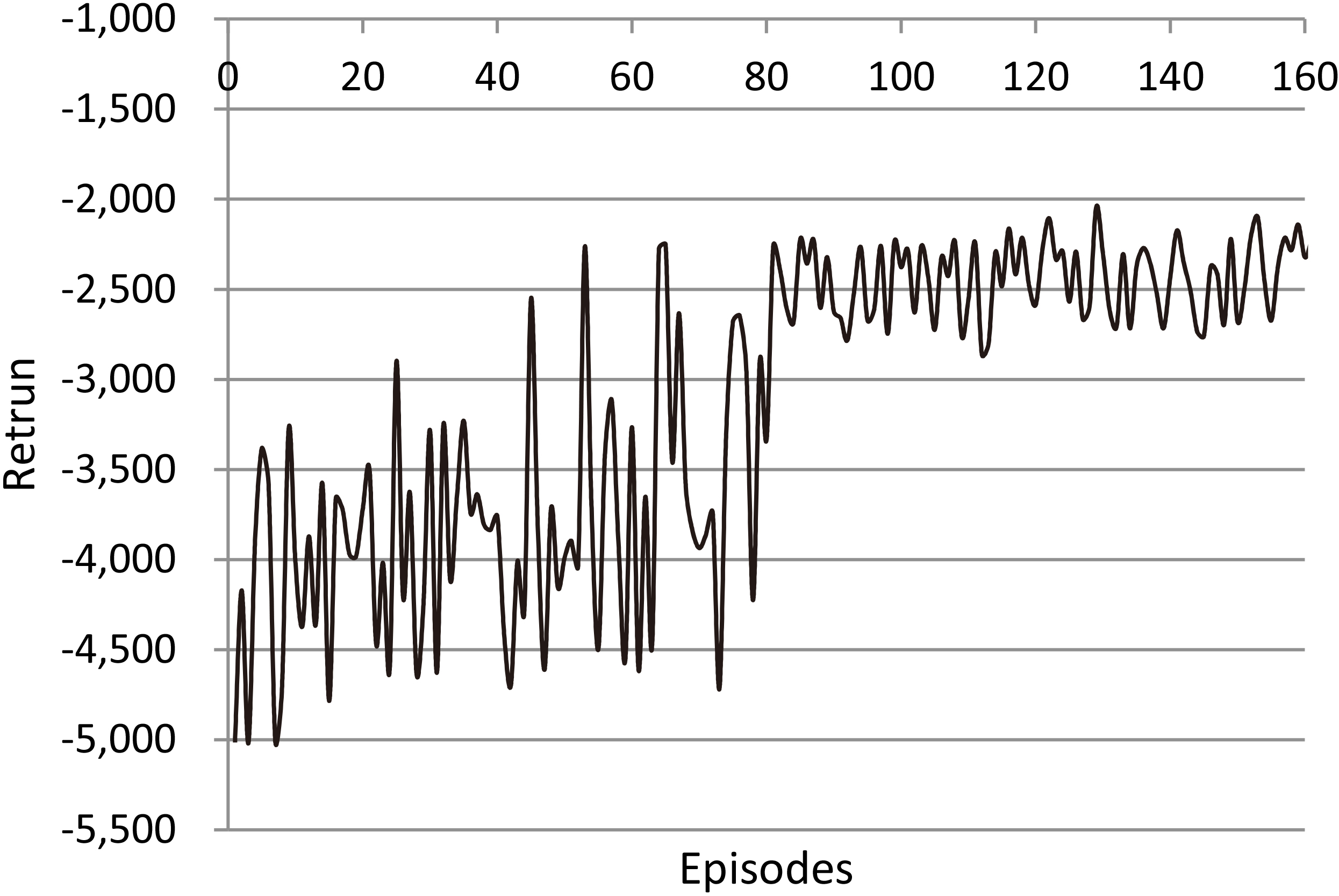
Return for the experiment 1 in 160 episodes.

Figure 3.

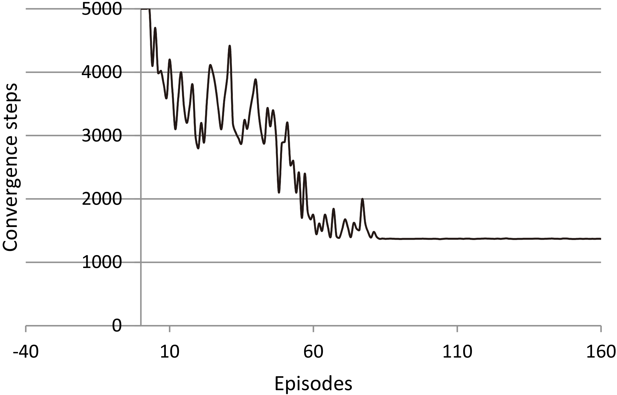
Steps to reach the optimal value for experiment 1 in 160 episodes.

Figure 2 is the average of the five groups of comparative experiments which show the change of return for each episode using the SAC in an experiment including 160 episodes. It is clear that return fluctuates much in the first 80 episodes with the maximum range of fluctuations is more than 3000. During this period, the agent is in the trial-and-error stage. And after 80 episodes, the return is stable at around $-$ 2500 and the maximum range of fluctuations is less than 500. Figure 3 is the average of the five groups of comparative experiments which shows the steps to reach the optimal value of each parameter during 160 episodes. In the first several episodes, the SAC can not reach the optimal value and stay stable around this value in 5000 steps; from 10 to 50 episodes, the SAC can do it between 4000 and 2000 steps; and from 50 to 80 episodes, the SAC can reach the optimal value and stay stable around this value in about 1500 steps. After 82 episodes, the steps to reach the optimal value and stay stable around this value of each parameter at around 1370 steps. The SAC learns through 82 episodes and finally converges in 1370 steps.

4.2 A comparative experiment on energy-saving performance

In experiment 2, we set the same initial state $s_{0}=$ [30, 770, 35, 20] for experiment 2.1 and 2.2, and $s_{0}=$ [10, 850, 15, 26] for experiment 2.3 and 2.4. But there is a difference between these sub experiments – the reward function weight $w=$ [0.05, 0.7, 0.1, 0.15] of experiment 2.1 and 2.3; the other reward function weight $w=$ [0, 0.7, 0.1, 0.2] of experiment 2.2 and 2.4. Table 1 shows the results as follows: although the average energy consumption in experiment 2.1 is 27441.3, which is more than 26355.6 in experiment 2.2 before convergence. After system converges, the energy consumption in experiment 2.1 falls to 21172.0, which is fewer than the one in experiment 2.2. From the long-term energy-saving aspects of consideration, the experiment 2.1 (which considers the energy consumption parameter) can better fit the goal of energy conservation than the experiment 2.2 (which does not consider the energy consumption parameter). Contrasting experiment between experiment 2.3 and experiment 2.4, which can better reflect the energy-saving of the SAC. Whether it converges or not, the average real-time energy consumption of experiment 2.3 is lower than the energy consumption in experiment 2.4. The result proves that the SAC with considering energy consumption parameter can effectively achieve the purpose of energy conservation.

Table 1
Performance analysis for SAC on energy-saving

Experiment	Initial state	Reward function	Convergence	Convergence	Average real-time energy consumption
number		weight $w$	steps	episodes	Before convergence	After convergence
2.1	[30, 770, 35, 20]	[0.05, 0.7, 0.1, 0.15]	1370	82	27441.3	21172.0
2.2	[30, 770, 35, 20]	[0, 0.7, 0.1, 0.2]	1370	82	26355.6	22904.8
2.3	[10, 850, 15, 26]	[0.05, 0.7, 0.1, 0.15]	1500	75	28660.3	25287.1
2.4	[10, 850, 15, 26]	[0, 0.7, 0.1, 0.2]	1500	75	30148.1	26177.9

5. Conclusions

With respect to the problem that the traditional control method has the disadvantages of slow convergence and instability in the control of building-related equipments, the Sarsa-based adaptive controller (SAC) is proposed. The SAC controller uses Sarsa algorithm, modeling the real housing air conditioning system, ventilation system and other related equipment constructions as a MDP, and consider the energy-saving factors. The input of SAC is the matrix representation of four states: indoor temperature, indoor CO ${}_{2}$ concentration, indoor relative humidity, and the setting temperature. The output of SAC is the permutations of actions of the air conditioning, the ventilation system, the humidifier and the dehumidifier. The purpose of SAC is to guarantee the achievement of the desired temperature, humidity and carbon dioxide concentration on the energy-saving effect. We set two comparative experiments both including 160 episodes with 5000 steps in each episode. The experimental results show that: Firstly, SAC can achieve good convergence and stability; secondly, SAC has an effective energy-saving; thirdly, reinforcement learning algorithm for building-related equipment control field has better convergence performance and robustness comparing with the PID method.

Footnotes

Acknowledgments

This research was partially supported National Natural Science Foundation of China (61502329, 61772357, 61750110519, 61772355, 61702055, 61672371, 61602334, 61502323, 61472262, 61472267), Natural Science Foundation of Jiangsu (BK20140283, BK2012616), Primary Research and Development Plan of Jiangsu Province (BE2017663), High School Natural Foundation of Jiangsu (13KJB520020), Key Laboratory of Symbolic Computation and Knowledge Engineering of Ministry of Education, Jilin University (93K172014K04, 93K172017K18), Suzhou Industrial Application of basic research program part (SYG201422).

Conflict of interest

We declare that there is no conflict of interest regarding the publication of this article.

References

Birchall

Gustafsson

Wallis

et al., Survey and simulation of energy use in the European building stock, in: Proc of 12th REHVA World Congress CLIMA 2016, 2016.

Allouhi

Fouih

Y.E.

Kousksou

et al., Energy consumption and efficiency in buildings: current status and future trends, Journal of Cleaner Production 109 (2015), 118–130.

Ulpiani

Borgognoni

Romagnoli

et al., Comparing the performance of on/off, PID and fuzzy controllers applied to the heating system of an energy-efficient building, Energy and Buildings 116 (2016), 1–17.

Kolokotsa

Tsiavos

Stavrakakis

G.S.

et al., Advanced fuzzy logic controllers design and evaluation for buildings’ occupants thermal-visual comfort and indoor air quality satisfaction, Energy and Buildings 33(6) (2001), 531–543.

Collotta

Tirrito

and Bobovich

A.V.

, Transmission amplitude management in power line communications through a fuzzy logic controller: A real case study, Journal of Computational Methods in Sciences and Engineering 16(1) (2016), 3–19.

Rafsanjani

M.K.

and Samareh

, Chaotic time series prediction by artificial neural networks, Journal of Computational Methods in Sciences and Engineering 16(3) (2016), 599–615.

Ben-Nakhi

A.E.

and Mahmoud

M.A.

, Energy conservation in buildings through efficient A/C control using neural networks, Applied Energy 73(1) (2001), 5–23.

Egilegor

Uribe

J.P.

Arregi

et al., A fuzzy control adapted by a neural network to maintain a dwelling within thermal comfort, Building Simulation 2 (1997), 87–94.

Dalamagkidis

Kolokotsa

Kalaitzakis

et al., Reinforcement learning for energy conservation and comfort in buildings, Building and Environment 42(7) (2007), 2686–2698.

10.

Fazenda

Veeramachaneni

Lima

et al., Using reinforcement learning to optimize occupant comfort and energy usage in HVAC systems, Journal of Ambient Intelligence and Smart Environments 6(6) (2014), 675–690.

11.

Yang

Nagy

Goffin

et al., Reinforcement learning for optimal control of low exergy buildings, Applied Energy 156 (2015), 577–586.

12.

Sutton

R.S.

and Barto

A.G.

, Reinforcement learning: an introduction, MIT Press, 1998.

13.