A critical-path focus for earned duration increases its sensitivity for project-duration monitoring and forecasting in deterministic,fuzzy and stochastic network analysis

Abstract

Earned duration metrics improve project-duration-performance monitoring and forecasting compared to earned schedule metrics because they depend only on time-based variables. In projects with multiple-parallel paths of work items and with work items varying significantly in individual durations, earned duration metrics sometimes fail to provide reliable project-duration monitoring and forecasts. Calculating earned duration using information for the critical-path work items only, provides a way of overcoming distortions in earned duration caused by non-critical-path work items. Weighting the work items used in an earned duration calculation, according to their individual-planned durations, places more emphasis on the longer-duration work items, which often constitute the more-crucial work items in terms of uncertainty and performance. Two new earned duration formulations are derived and evaluated. The analysis is performed using deterministic, stochastic and fuzzy models related to work breakdown progress diagrams that illustrate the quality and reliability of the information that can be derived from these new formulations.

Keywords

Earned duration stochastic project analysis fuzzy EVM critical-path analysis duration performance index DPI quantified project risk analysis

1. Introduction

Earned Value (EV) analysis evolved as a cost-management technique [5] to become an established project monitoring and forecasting tool [2, 11] recommended by the Project Management Institute [24, 25]. The EVM framework incorporates project cost and duration performance indicators, but its cost-derived schedule performance indicator (SPI) does not provide reliable to-completion forecasts [7, 14]. The proposed the Earned Schedule (ES) metric [12] and the time-based schedule performance indicator (SPIt) to provide more reliable to-completion project duration forecasts (PPDt) are now accepted as part of EVM’s project-duration-monitoring. It is not without its drawback though as it remains cost-derived and it becomes less reliable in project networks with multiple parallel paths of work items [27].

Khamooshi and Golasfhani [10] proposed the calculation of earned duration (ED) and the duration performance indicator (DPI) derived only from time-based variables to provide more reliable project-duration-performance monitoring and to-completion forecasting than ES and SPIt. Batselier and Vanhoucke [3] concluded, based on analysis of many projects, that ED-DPI provided slightly more reliable to-completion duration forecasts than ES-SPIt (to quote Bastelier and Vanhoucke [3, p. 1505]: “…the overall results of our study show a slight advantage of EDM(t)-DPI over ESM-SPI(t)…”). That to-completion-forecasting advantage does depend though on their EDM(t-1) calculation improving upon the accuracy of ESM(t-1). They also noted that neither of the metrics worked well for all projects, and that improvements and refinements to both methods were required.

EVM analysis is typically applied in deterministic calculations that fail to consider uncertainties associated with work items yet-to-be delivered, or with the quality of information available for in-progress work items. Stochastic methodologies have been proposed to provide risk-adjusted EVM analysis [28, 1]. Fuzzy logic models can also overcome some of the deterministic limitations of EVM analysis by incorporating uncertainties concerning the quality of information available about the status of work items at specific points in time [23, 21, 22, 32].

EVM sometimes fails to provide accurate duration performance monitoring and can be difficult to apply [19]. Hazir [6] considers EVM’s two-dimensional-cost-duration focus a weakness and highlights the need to also take into account operational, technical and quality factors and uncertainties to improve project performance analysis. It has been noted [29, 17] that as project networks involve more parallel pathways ES-based forecasts to-completion frequently worsen, but claims that situation can be overcome by modifying the earned schedule method to calculate a more complex “Longest Path” method.

This author believes that project performance monitoring via EVM can be improved by focusing more attention on “critical-path” work items, in particular on the more “crucial” work items located on the critical path; and, that earned duration metrics can be adapted to provide such a focus. Section 2 describes the derivation of ES and ED metrics and justifies the benefits of calculating two novel ED metrics, focused on critical-path work items (EDcp) and those critical-path work items weighted for their planned durations (EDcpwt), placing more emphasis on “crucial” work items. Section 3 provides analysis of an example multiple-pathway project using deterministic, stochastic and fuzzy models to demonstrate how the novel proposed ED metrics add additional dimensions to project-duration-performance monitoring and forecasting. Appendix 1 lists definitions of the EVM-related metrics referred to in this study.

2. Earned duration: Justifications for alternative computations

2.1 Potential drawback associated with Earned schedule (ES)

Earned schedule (ES) is an established metric providing reliable schedule performance monitoring and to-completion duration forecasting for the majority of projects. ES is calculated incrementally across a series of time intervals [12] along the baseline planned schedule (BSP), and Eq. (1) is one way to express the calculation of ES at any time point $x$ (ES ${}_{x}$ ) along the BPS:

${}_{x}=$ (1) ${}_{t}+$ ${}_{x}$ ${}_{t})$ ${}_{t+1}$ ${}_{t}))$ $\Delta$

where, ES ${}_{x}$ is earned schedule at time point $x$ and ES ${}_{t}$ is earned value previously earned at the earlier time point $t$ . EVx is the earned value at time point $x$ , at which point PV ${}_{t}$ $<=$ EV ${}_{x}$ $<$ PV ${}_{t+1}$ . PV is the planned value at time point $t$ (PV ${}_{t}$ ) and the later time point $t+1$ (PV ${}_{t+1}$ ). EV and PV metrics are expressed in cost units. $\Delta$ T is the planned time interval between time point $t$ and time point $t+1$ . Hence, ES and $\Delta$ T are expressed in calendar time units (e.g. days, weeks, months, etc.), but the other variables in Eq. (1), EV and PV, cost based.

Equation (1) differs from the formula originally applied to ES based upon a project being broken down into equal planned time increments [15], which was also adopted as standard for ES calculation by the PMI [25] and shown here as Eq. (2).

$=$ (2) $+$

where, $C$ is the number of whole time increments of the performance measurement baseline (the cumulative planned value, PV, over time) where the condition EV $>=$ PV is met (i.e. earned value already earned); “I” is (EV -PVc)/(PVc+1 – PVc), where “c” refers to a count number of the periods involved. Equation (1), or equivalents to it, are widely used [8, 9, 10], because it provides ES in absolute time units rather than in terms of numbers of time increment (c), or fractions of increments of the time schedule earned. It is Eq. (1) that is preferred and used in this study for project schedules that are planned and evaluated in absolute time units (i.e. days, weeks, months, etc.).

The ES calculation essential makes the assumption that the schedule is progressing between time points “ $t$ ” and “ $t+1$ ” at the same rate as costs are progressing. In most projects there is a strong positive correlation between work item durations and their costs, so this assumption is valid and the ES calculation is reliable. However, as Khamooshi and Golasfhani [10] point out this is not always the case. For instance, some projects involve one or more short-duration-but-high-cost work items, relative to the majority of the project’s work items, resulting in a breakdown in the correlation between cost progress and duration progress at certain points along the BPS. The magnitude of such errors inherent in linear interpolation between time point “ $t$ ” and “ $t+1$ ” is project specific. It tends to be small for those projects in which cost and time are strongly correlated for the all work items, and, in such cases, tends to decrease and become less influential on forecasts as the number of time increments considered increases.

2.2 Earned Duration (ED) avoiding cost-derived variables

The calculation of earned duration was originally described by Jacob and Kane [9] to be calculated independently of costs. Khamooshi and Golasfhani [10] refined the calculation of earned duration (ED) independently of work-item costs and based only on work item durations. They proposed that ED be calculated following a similar methodology to that used for ES. Hence, ED is also calculated incrementally across a series of time intervals along the baseline planned schedule (BSP), and Eq. (3) is an alternative method to that proposed by Khamooshi and Golasfhani [10] to express the calculation of ED at any time point x (ED ${}_{x}$ ) along the BPS:

${}_{x}=$ (3) ${}_{t}+$ ${}_{x}$ ${}_{t})$ ${}_{t+1}$ ${}_{t}))$ $\Delta$

where, ED ${}_{x}$ is earned duration at time point $x$ and ED ${}_{t}$ is earned duration previously earned at the earlier time point $t$ . APCx is the percentage of the project actually completed at time point $x$ along the BPS, at which point PPC ${}_{t}$ $<=$ APC ${}_{x}$ $<$ PPC ${}_{t+1}$ . PPC ${}_{t}$ and PPC ${}_{t+1}$ are the percentages of the project planned to be completed at time point $t$ and the later time point $t+1$ , respectively. $\Delta$ T is the planned time interval between time point $t$ and time point $t+1$ . Hence, all components of the ED calculation are expressed in percentages or calendar time units (e.g. days, weeks, months, etc.) and are independent of costs.

APCx can be calculated by Eq. (4):

$\displaystyle\textit{APCx}=\left({\mathop{\sum}\limits_{i=1}^{n}f_{i}}\right)/n$ (4)

where, $n$ is the total number of work items involved in the project, and $f_{i}$ is the fraction of work item “ $i$ ” that is completed at time point $x$ . “ $f_{i}$ ” can vary from “0” for a work item not yet started to “1” for work items completed, and will be fractions between “0” and “1” for work items in progress.

ED can be used to calculate the duration performance index (DPI) using Eq. (5):

$=$ (5)

where, AD is actual duration at the same time point $x$ at which ED is calculated.

2.3 Earned duration focused on critical path work items (EDcp)

For projects with multiple parallel pathways of work items, it is proposed that the earned duration calculation can be usefully modified to calculate the earned duration for critical path work items only (EDcp). Focusing on critical-path work items only to derive EDcp and DPIcp is considered to be particularly appropriate for high-level project networks, or projects comprised of relatively few work items with varying durations and multiple parallel pathways. In such networks, it is possible in some scenarios for delayed or slow performing critical items to become diluted in their impact on the standard ED metrics Eqs (3) to (5) by completion of parallel-but-non-critical work items. Considered a project including three work items A, B and C executed in parallel at a certain interval of the BPS with the critical path potentially switching among, them depending upon the actual input duration values assigned to each of the work items. In certain scenarios within certain time intervals of the BPS, the two non-critical items (e.g., A and C) may be rapidly completed, but the critical work item B could be delayed. This would lead to the calculated ED and DPI values being over optimistic (i.e., too high) and potentially underestimating the remaining time to project completion. Calculating EDcp and DPIcp for the critical-path work items only potentially avoids this potential problem. Such situations are only likely to affect some project scenarios, but they can be identified by monitoring for significant differences in ED and EDcp values along the BPS.

APCxcp can be calculated by Eq. (6):

$\displaystyle\textit{APCxcp}=\left({\mathop{\sum}\limits_{i=1}^{k}f_{icp}}% \right)/k$ (6)

where, $k$ is the total number of work items on the critical path involved in the project, and $f_{icp}$ is the fraction of critical-path work item “ $i$ ” that is completed at time point $x$ . “ $f_{icp}$ ” can vary from “0” for a work item not yet started to “1” for work items completed, and will be fractions between “0” and “1” for work items in progress. Equation (2) can then be used to calculate EDcp with APCxcp replacing APCx and with the PPC components replaced by PPCcp representing percentages of the project completed based upon the planned critical path work items only.

EDcp can be used to calculate the critical-path duration performance index (DPIcp) using Eq. (7):

$=$ (7)

2.4 Earned duration incorporating weightings for planned work-item durations

In order to improve the reliability of EDcp as a project monitoring and forecasting indicator in cases where critical path work items display a wide range of individual durations, it is further proposed that the EDcp calculation is weighted by the planned durations of the critical path work items to calculate EDcpwt. In a project with a small network of work items (e.g., $<$ 25 or so) the relative durations of each work flow item can have a distorting impact on ED and EDcp calculated at certain points along the BPS. It is not uncommon for individual work item durations to vary by more than a factor of 5. The impact on project duration uncertainty of delays in starting long-duration critical path work items can be underestimated in ED and EDcp calculations. The basic calculation of APCx Eq. (4) involves dividing the sum of the fractions of work items completed at time point $x$ and dividing it by the total number of work items in the project ( $n$ ). Whereas, the short-duration work items may be completed within relatively few of the time intervals used to calculate ED, the longer-duration work items may take several time intervals to complete. In intervals where multiple parallel items are in progress but progressing slowly, the earned duration progress of the project is likely to be slow in that interval. Such a problem can be exacerbated in the APCxcp calculation Eq. (6) where the denominator $k$ (total number of critical path work items) is much less than $n$ . Also, in situations where a number of short-duration work items are completed early in the critical path progress towards completion can appear to be more rapid not taking into account the long-duration items to follow, which will progress over several time intervals towards completion.

The EDcpwt metric involves weighting each work item by the planned duration time for that work item in the calculation of APCxcpwt Eq. (8). For example, in a project with ten work items summing to a total of 150 days, with five critical items on the critical path with total work item planned durations summing to 100 days, the denominator for calculating the actual percentage of project schedule completed (APCxcpwt) at point $x$ would be “100”. However, if one of the critical path work items involved 40 days duration and another involved 15 days duration, their respective contributions to APCxcpwt would be 40/100 and 15/100, respectively, rather than each contributing 1/5 to the calculation of APCxcp.

$\displaystyle\textit{APCxcpwt}=\left(\sum^{k}_{i=1}(f_{icp}xD_{ipcp})\right)/% \sum^{k}_{i=1}D_{ipcp}$ (8)

Where, $D_{ipcp}$ is the planned duration of critical path item $i$ . Equation (3) can then be used to calculate EDcpwt with APCxcpwt replacing APCx and with the PPC components replaced by PPCcpwt representing percentages of the project completed based upon the planned critical path work items only weighted for their respective planned durations.

EDcpwt can be used to calculate the critical-path-weighted duration performance index (DPIcpwt) using Eq. (9):

$=$ (9)

Applying the duration-weighted method (Eqs (3), (8) and (9), in that order) removes the potential distortions caused by critical-path work items of significantly different durations distributed at different points along the BPS. The relative contribution of the duration of each work item to the total duration of all work items on the critical path should be taken into account when evaluating a project [26]. Williams [30] termed this attribute “cruciality” and pointed out delays and uncertainties associated with “highly-crucial” work items have more significant influences on project performance and uncertainty than less crucial work items. The calculations of EDcpwt and DPIcpwt essentially attribute more weight to the more-crucial work items along the critical path than the ED or EDcp metric. EDcpwt and DPIcpwt should, therefore, respond more positively when highly-crucial (long-duration) work items are started early and/or finished early, and, respond more negatively if they are started late and/or finished late. Such responses are considered appropriate based on the levels of uncertainty associated with such outcomes.

It is useful to compare the values of three distinct ED metrics and their derivative DPIs, as defined in equations by Eqs (3) to (9) with ES and SPIt at various time intervals across the BPS. The calculations of all these metrics discussed can be usefully included in deterministic, stochastic and fuzzy cost-time project analysis, either separately or as part of integrated models including all three types of analysis. In order to demonstrate this, the proposed metrics are calculated along the BPS of an example project, displayed in the form of a work breakdown progress diagram (WBPD), and the results analyzed in some detail with the network algorithms and metric calculations performed by Excel models driven by VBA macros.

3. Critical-path duration analysis applied to an example project

An integrated deterministic, fuzzy and stochastic analysis (see Appendix 2 for definitions of these types of calculations) is described for a project to construct a production plant. It is a large-scale, long-term project broken down into twenty high-level work items that are executed across five pathways, involving periods of parallel engineering conducted across two or more pathways. Depending upon the individual work item durations applied the example project’s critical path may switch from one pathway of work items to another. The critical pathway for the remainder of a project yet-to-be completed may not be the critical pathway that has prevailed up to the stage of the project so far completed [13] and can in some cases become a shorter path and no longer “the longest path” [16], and may not necessarily be best estimated by the earned schedule method [8, 20]. However, for whatever duration assumptions that are made for individual work items in a particular case, one pathway will always constitute the critical path (or longest path) for that case.

3.1 Description of example project in terms of duration and schedule

Table 1 provides work-item-duration assumptions for three deterministic cases (i.e., best estimate, low and high cases) used to evaluate the example project. These three case assumptions are also used to define input cost and duration distributions (e.g., lognormal, normal, triangular, and uniform) for each work item to be sampled randomly by a stochastic model (i.e. low case used as the tenth percentile (P10); Best estimate used as modal value; and, the high case used as the ninetieth percentile (P90)).

The right side of Table 1 provides the network logic relationships applied among the work items (Fig. 1), with the numerical values shown representing work item numbers. This network logic and precedence rules are used to establish an algorithm applied to deterministic, fuzzy and stochastic models for determining at what point in the schedule each work item can start. Crucially, and unique to each project/arrangement of work items, it identifies the convergent and divergent points within the network. Time taken by preceding work items to reach the convergent points determines which of the parallel paths of work items constitutes the critical path. Work items 7, 8, 17, 18 and 20 are convergent points in the example project’s network; two or more lower-numbered work items converge into those convergent points and must be completed before activity at the convergent point can commence.

The network logic (Table 1 and Fig. 1) is used to develop the network algorithm used for both deterministic and stochastic models. The algorithm used to determine the project schedule for each set of work-item duration assumptions performs forward and backward passes sequentially applying the defined network logic. This leads to the determination of five time-related values associated with every work item, given the input duration (D) assumption for each work item associated with either a deterministic or stochastic case. These values are: earliest start (ESt); earliest finish (EF); latest start (LSt); float (F); and latest finish (LF).

Table 1
Network logic for example production plant construction project work items

Project work breakdown into 20 work items		Parallel work-item	Work items of a specified parallel path that must be complete before a
implemented across 5 parallel paths		path identifier	subsequent work item in column 1 can begin
Work item number	Work item description	(A to E)	A	B	C	D	E
1	Market/Economic Model/Business Case	A
2	Short-list Potential Products	B	1
3	Feasilibility Study	B		2
4	Select Product Mix	B		3
5	Short-list Potential Locations	C	1
6	Negotiate Land Fees with Land-owners	C			5
7	Obtain Planning Permissions	C		3	6
8	Finalize Site Selection	A		4	7
9	Detailed Design/Process Eng.	A	8
10	Contract and Construct Plant Buildings	B	9
11	Install Product Line X	B	10
12	Install Product Line Y	A	10
13	Install Product Line Z	C	10
14	Construct Administration Offices	D	9
15	Recruit Operating Staff	E	9
16	Develop Marketing Network	E					15
17	Install Safety and Control Systems	A	12	11	13
18	Train Staff	A	17			14	15
19	Setup Distribution Systems	E					16
20	Test, Hook-up and Commission	A	18				19

Work items # 7, 8, 17, 18 and 20 are convergent points in the network with two or more other work items feeding directly into them.

Figure 1.

Arrow-on-node diagram of the project network for the twenty high level work items of the example project with the critical path for the best-estimate (planning) case highlighted.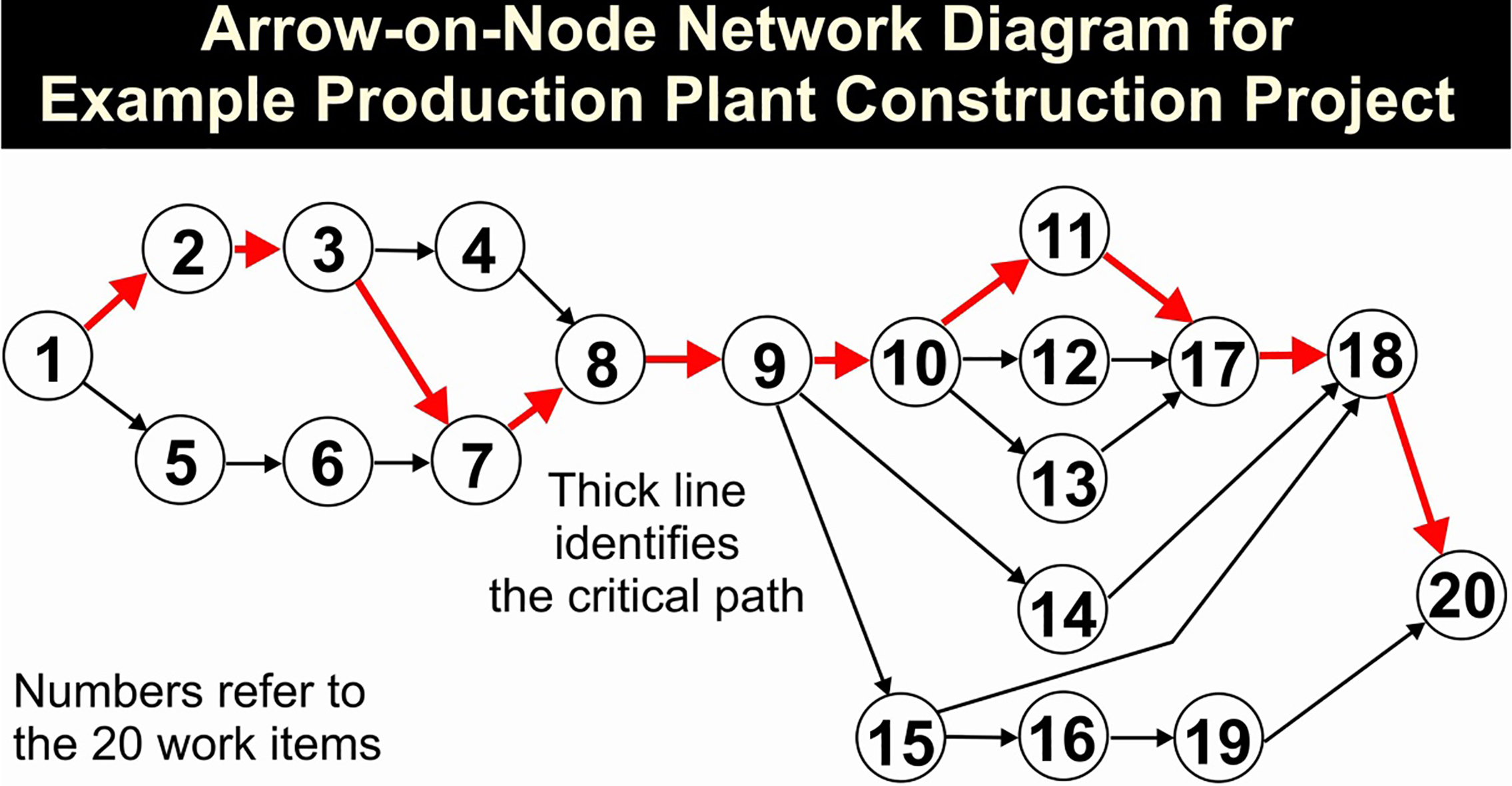

3.2 Duration analysis of example project scenarios

The best-estimate duration assumptions and the work schedule calculated for that scenario are taken as the “planned” or “baseline” schedule for the example project. Table 2 shows percentages of work items completed at specified intervals along the baseline planned schedule (BPS), expressed as percentages of the completed-project planned duration (PD), i.e., the best estimate case assumptions for the example project. The low-case scenario completes within 75% of PD, whereas the high-case scenario does not complete until approximately 135% of PD. The 5% intervals are displayed to provide a high-level comparison of the deterministic cases and planned scenarios considered. By weighting the planned projects critical path work items for their durations (last column Table 2), the percentages of the project completed match the percentage intervals of the BPS. Evaluating project performance at regular intervals along BPS is considered a useful method for monitoring and modelling project performance and forecasting indices derived for a range of scenarios at the project planning stage.

The work breakdown schedule and duration network for the project could be usefully illustrated, for each scenario considered, as either a precedence or arrow-on-node diagram (Fig. 1). Additionally, a work breakdown schedule progress diagram (WBPD) is displayed (Fig. 2) for the high-case duration assumptions from Table 1 for each work item at 5% intervals of PD, with the critical path items highlighted (i.e., red thick line). Work items that have not yet started are shown (Fig. 2) as “0”, those completed as “1”, and those in progress as a fraction of work completed. Important schedule information for each work item, calculated by the schedule algorithm applied, is listed in columns 2 to 5 (Fig. 2). The critical path items are those with “0” float (column 3). An assumption made for scheduling in each scenario presented is that the non-critical-path items are commenced once 50% of the float has elapsed.

Figure 2 shows which work items are completed, or partially completed, at each specified time period along the planned duration. The “1’s” and fractional numbers are added for each of columns 6 to 25 in Fig. 2 to provide the number of work items competed at each point along the BPS (last-but-one row in Fig. 1); a number that is divided by the total number of work items in the project (i.e., 20 in the example project) to provide the fraction of the project completed, expressed as a percentage in the last row of Fig. 2. A comparison of the last row percentages with the top row percentages (the BPS) reveals the high-case scenario is significantly behind the planned schedule from the outset. The percentages of all work items completed at each specified time along the BPS are used to calculate earned duration and derivative metrics.

Table 2
Deterministic case and planned schedule outcomes for example production plant construction project considered

	Actual percentages of project completed (APC) at various points along the baseline project schedule (BSP)
	Deterministic cases			Planned schedules
Percentage of	Best estimate	Low estimate	High estimate	Planned percentage	Planned percentage	Planned percentage
baseline planned	case (Adopted	case (P10 values	case (P90 values	of project’s	of critical path	of weighted
schedule’s time	as planned	of all work-item	of all work-item	work items	completed	critical path
elapsed (BSP)	schedule)	distributions applied)	distributions applied)	completed PPC	PPCcp	completed PPCcp
5%	2.58%	3.88%	1.94%	2.58%	4.70%	5%
10%	5.50%	17.50%	3.88%	5.50%	10.00%	10%
15%	16.46%	25.38%	7.17%	16.46%	20.15%	15%
20%	22.92%	34.25%	15.94%	22.92%	24.85%	20%
25%	26.25%	41.88%	20.78%	26.25%	29.55%	25%
30%	33.83%	45.30%	24.75%	33.83%	34.24%	30%
35%	39.25%	46.85%	27.02%	39.25%	44.09%	35%
40%	42.33%	50.66%	33.63%	42.33%	49.70%	40%
45%	44.92%	61.04%	36.50%	44.92%	54.39%	45%
50%	46.25%	85.42%	40.63%	46.25%	56.82%	50%
55%	47.54%	89.29%	42.56%	47.54%	59.17%	55%
60%	52.44%	95.33%	44.50%	52.44%	61.52%	60%
65%	61.95%	97.27%	45.72%	61.95%	64.45%	65%
70%	83.16%	99.21%	46.69%	83.16%	72.83%	70%
75%	87.64%	100.0%	47.66%	87.64%	77.53%	75%
80%	90.50%		51.58%	90.50%	82.73%	80%
85%	95.35%		58.51%	95.35%	91.55%	85%
90%	96.90%		72.30%	96.90%	94.36%	90%
95%	98.45%		84.56%	98.45%	97.18%	95%
100%	100.0%		87.50%	100.0%	100.0%	100%
105%			89.44%
110%			93.30%
115%			95.82%
120%			97.11%
125%			98.40%
130%			99.69%
135%			100.0%	20 work items	11 work items	11 work items

Note: Shaded rows are the points along the BPS for which detailed analysis is presented.

Figure 2.

Work-breakdown-progress diagram (WBPD) for the High-case assumptions derived from the network logic and expressed at 5% intervals of the planned duration (best-case estimate to-completion estimate) forming the BPS. Critical-path work items are highlighted with a thick (red) outline. This high-case scenario does not complete until 135% of the planned schedule (i.e. it finishes very late with respect to the planned schedule). Note parallel work items 11 and 12 in this case have the same durations and are both critical path items. There are therefore 12 critical path items it this case compared to 11 in the best estimate and most other scenarios evaluated.

Consideration of the work items completed and costs incurred, for each scenario evaluated at each time increment relative along the BPS, enable an array of earned value (EV), earned schedule (ES) and earned duration (ED) metrics to be derived. Tables 3 and 4 provide selected EV-ES-ED metrics for the three deterministic cases and the mean values of those metrics from a 1000-run Monte Carlo simulation constituting the stochastic model.

The EV and ES metrics displayed in Table 3 are those that are widely used to monitor project performance and to forecast to-completion values of project cost and duration. The metrics included in Table 4 are those related to earned duration including the ones proposed in this study that focus upon critical path work items only. Tables 3 and 4 provide comparisons of the EVM to-completion and project criticality indices based on EV-, ES-, ED- and ED critical-path-derived metrics.

Four informative project criticality ratios are displayed in the last four columns of Table 4 and these are useful for providing an integrated cost-duration index monitoring the health and viability of a project in terms of achieving its combined cost and schedule targets. A CR ratio (CPI multiplied by SPIt and derived from earned-schedule calculations) of equal to or greater than 1 should generally indicate that a project is able to achieve its targets. However, scenarios arise with one of the component indices (CPI or SPIt) being $>$ 1 and the other being $<$ 1, but still yielding a CR of $>$ 1. For this reason Cioffi [4] proposed the more-complex-to-calculate (see appendix) cost schedule performance factor (CSPF), which yields values of $>$ 1 for projects that have either CPI or SPI below 1. Modifications of these two project-criticality indices using the duration performance index for just critical-path work items (DPIcp and DPIcpwt) for estimating schedule, in place of SPIt, are also shown in Table 4 as CRcpwt and CSPFcpwt.

The critical path only metrics are derived using the work breakdown progress diagram displayed as Fig. 3, rather than Fig. 2, for the high-case duration assumptions from Table 1 for each work item at 5% intervals of PD, with the critical path items highlighted by a thick line. In Fig. 3 all non-critical path work items are assigned “0” values at all time intervals across the BPS and do not contribute to the percentage-of-work-items-completed calculation. Also, for the critical path items, rather than changing from “0” to “1” as a work item is completed as in Fig. 2, they change from “0” to “number of planned days for that work item” (Fig. 3, Table 1), applying planned duration weightings to each work item. For the high-case scenario, the different calculations leading to the calculated percentages of project completed (last rows in Figs 2 and 3) result at 45%PD, 60%PD and 85%PD in quite different outcomes: 36.5%, 44.5% and 58.5%, respectively for Fig. 2, compared to 31.7%, 42.2% and 60%, respectively, for the weighted-critical-path calculation (Fig. 3). The weighted calculation assigns more weight to long-duration-critical-path work items #9 and #10; as those work items are delayed in starting relative to the plan in the high-case scenario, the earned duration (EDcpwt) for pre-45%PD interval based on the weighted calculations are lower than for the unweighted calculations.

A comparison of the ED versus EDcpwt and DPI versus DPIcpwt values in Table 4, across the three deterministic scenario evaluated, reveals that the critical-path-weighted metrics show more sensitivity, particularly at the earlier stages of the project (i.e., 20%PD and 40%PD. EDcpwt is higher than ED for the low-case (faster than planned), and lower than ED for the high-case (slower than planned) for stages 20%PD and 40%PD. Also DPIcpwt is higher than DPI for the low-case, and lower than DPI for the high-case. This greater sensitivity makes the critical-path-weighted metrics more useful for monitoring purposes in reflecting greater uncertainties associated with the performance of crucial work items. In this example project crucial work items #9 and #10 do not commence for the assumptions applied until after 35% of the project is completed. It is therefore appropriate that duration performance indices calculated at times before 35% of the project is completed reflect greater uncertainty in the performance of crucial work items that have not yet begun.

Table 3

Earned value and schedule calculated values and indices for deterministic and stochastic cases of example production plant construction project considered

Deterministic case descriptions	Actual	Earned	Cost	CPI-based	Schedule	SPI-based	Earned	Schedule	SPIt-based
(best estimate case used as	project	value	performance	projected	performance	projected	schedule	performance	projected
planned schedule and budget)	cost at a	($ millions)	index	project cost	index	project	(days)	index (time	project
	specified			at completion	(cost based)	duration at		based/cost	duration at
	% of PD			($ millions)		completion		derived)	completion
	($ millions)					(days)			(days)
Metric abbreviation	AC	EV	CPI	PCaC	SPI	PPD	ES	SPIt	PPDt
Best Estimate Case @20% of PD	133.5	133.5	1.000	992.4	1.000	930	186	1.000	930
PD $=$ Planned Duration
Best Estimate Case @40% of PD	223.3	223.3	1.000	992.4	1.000	930	372	1.000	930
Best Estimate Case @60% of PD	490.6	490.6	1.000	992.4	1.000	930	558	1.000	930
Best Estimate Case @80% of PD	948.8	948.8	1.000	992.4	1.000	930	744	1.000	930
Best Estimate Case @100% of PD	992.4	992.4	1.000	992.4	1.000	930	930	1.000	930
Low Estimate Case @20% of PD	123.2	183.6	1.490	666.2	1.375	676	284	1.529	608
Low Estimate Case @40% of PD	327.2	461.9	1.412	702.9	2.069	450	544	1.464	635
Low Estimate Case @60% of PD	681.7	956.2	1.403	707.5	1.949	477	790	1.415	657
Low Estimate Case @80% of PD	706.9	992.4	1.404	706.9	1.046	640	930	1.333	670
Low Estimate Case @100% of PD	706.9	992.4	1.404	706.9	1.000	670	930	1.333	670
High Estimate Case @20% of PD	49.3	29.9	0.608	1632.2	0.224	4145	127	0.685	1358
High Estimate Case @40% of PD	271.6	181.2	0.224	1486.9	0.812	1146	277	0.745	1248
High Estimate Case @60% of PD	367.3	247.9	0.675	1470.6	0.505	1841	411	0.737	1263
High Estimate Case @80% of PD	639.3	467.0	0.731	1358.4	0.492	1889	547	0.735	1265
High Estimate Case @100% of PD	1220.2	920.7	0.755	1315.3	0.928	1002	695	0.748	1244
High Estimate Case @120% of PD	1293.8	970.0	0.750	1323.6	0.977	951	843	0.756	1231
High Estimate Case @140% of PD	1326.7	992.4	0.748	1326.7	1.000	1220	930	0.741	1220
Mean of Simulation @20% of PD	135.4	128.9	0.980	1047.7	0.966	1247	198	1.066	904
Mean of Simulation @40% of PD	239.9	234.8	0.996	1016.1	1.051	904	381	1.023	924
Mean of Simulation @60% of PD	527.1	524.8	1.002	999.9	1.070	941	559	1.001	938
Mean of Simulation @80% of PD	922.4	926.0	1.009	988.7	0.976	959	739	0.993	943
Mean of Simulation @100% of PD	984.8	984.1	1.004	993.1	0.992	914	898	0.982	942

Table 4

Earned duration calculated values and indices for deterministic and stochastic cases of example production plant construction project considered

Deterministic case descriptions (best estimate case used as planned schedule and budget)	Earned duration (days)	Duration performance index (time based/ time derived)	DPI-based projected project duration at completion (days)	Earned duration critical path unweighted (days)	Earned duration critical path weighted (days)	Duration performance index (time based from critical path)	DPIcpwt- based projected project duration at completion (days)	Project critical ratio (CPI *SPIt)	Cost schedule performance factor	Project critical path ratio (CPI *DPIcpwt)	Critical path cost schedule performance factor
Metric abbreviation	ED	DPI	PPDed	Edcp	EDcpwt	DPIcpwt	PPDedcpwt	CR	CSPF	CRcpwt	CSPFcpwt
Best Estimate Case @20% of PD	186	1.000	930	231	186	1.000	930	1.000	1.000	1.000	1.000
PD $=$ Planned Duration
Best Estimate Case @40% of PD	372	1.000	930	462	372	1.000	930	1.000	1.000	1.000	1.000
Best Estimate Case @60% of PD	558	1.000	930	572	558	1.000	930	1.000	1.000	1.000	1.000
Best Estimate Case @80% of PD	744	1.000	930	769	744	1.000	930	1.000	1.000	1.000	1.000
Best Estimate Case @100% of PD	930	1.000	930	930	930	1.000	930	1.000	1.000	1.000	1.000
Low Estimate Case @20% of PD	283	1.519	612	325	287	1.540	604	2.278	0.338	2.294	0.336
Low Estimate Case @40% of PD	541	1.455	639	564	542	1.458	638	2.066	0.409	2.058	0.410
Low Estimate Case @60% of PD	790	1.416	657	851	790	1.416	657	1.985	0.424	1.986	0.424
Low Estimate Case @80% of PD	930	1.388	670	930	930	1.388	670	1.872	0.489	1.872	0.489
Low Estimate Case @100% of PD	930	1.388	670	930	930	1.388	670	1.872	0.489	1.872	0.489
High Estimate Case @20% of PD	137	0.738	1260	169	130	0.696	1336	0.416	1.460	0.423	2.228
High Estimate Case @40% of PD	278	0.747	1245	289	262	0.706	1318	0.497	1.951	0.471	1.973
High Estimate Case @60% of PD	411	0.737	1263	457	392	0.703	1324	0.497	1.927	0.474	1.947
High Estimate Case @80% of PD	550	0.739	1259	521	525	0.706	1318	0.537	1.735	0.516	1.820
High Estimate Case @100% of PD	696	0.748	1243	736	705	0.759	1225	0.564	1.671	0.573	1.648
High Estimate Case @120% of PD	843	0.756	1231	885	847	0.759	1225	0.567	1.665	0.569	1.663
High Estimate Case @140% of PD	930	0.763	1220	930	930	0.763	1220	0.554	1.696	0.554	1.696
Mean of Simulation @20% of PD	195	1.047	914	236	189	1.016	939	1.047	1.181	0.998	1.206
Mean of Simulation @40% of PD	382	1.027	921	464	379	1.018	929	1.021	1.124	1.015	1.129
Mean of Simulation @60% of PD	558	1.000	939	580	558	1.000	939	1.004	1.091	1.003	1.092
Mean of Simulation @80% of PD	741	0.996	940	772	737	0.991	946	1.003	1.073	1.000	1.077
Mean of Simulation @100% of PD	900	0.985	939	912	899	0.985	940	0.992	1.074	0.992	1.074

Figure 3.

Work-breakdown-progress diagram (WBPD) calculated for critical path work items only, weighted for best estimate (planned) work-item duration for the High-case assumptions derived from the network logic and expressed at 5% intervals of the planned duration forming the BPS. Critical-path work items are highlighted with a thick outline. This diagram should be compared with Fig. 1, which shows the same case but with all work-items considered and no weightings applied.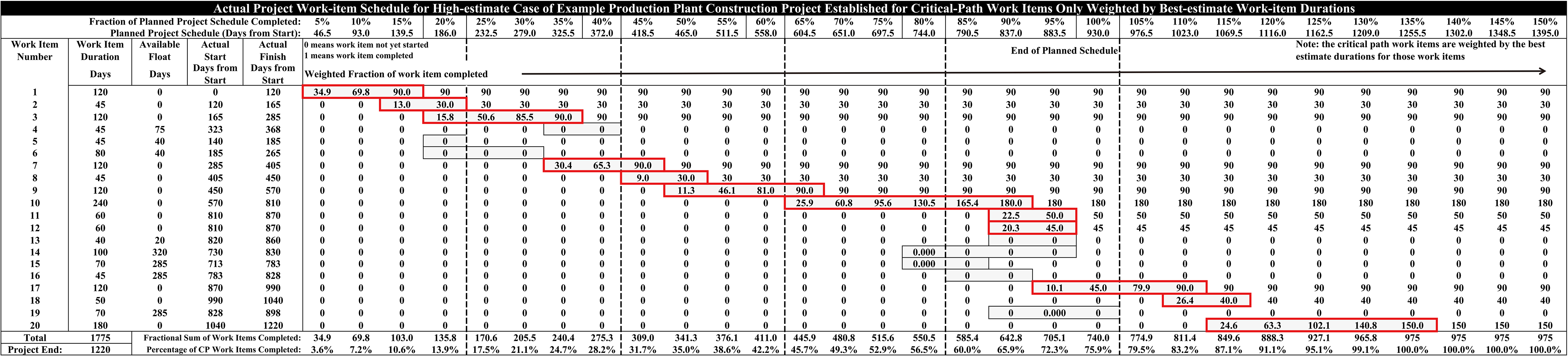

For other projects crucial work items may be positioned to start either earlier of later than for the example project considered. If they start later the critical-path-weighted duration metrics should be expected to show greater uncertainty for performance calculated at later stages (e.g. 60%PD or later). As each project has its own unique network schedule and distribution of critical and crucial work items, so it cannot be concluded that it is only the early estimates that would show significant differences in ED versus EDcpwt.

3.3 fuzzy analysis of example project scenarios

In order to apply a fuzzy model to reflect potential uncertainties associated with the degree of completion of each work item at any stage along the WBPD the calculated fractions completed (e.g. as shown in Figs 2 and 3) were transformed into trapezoidal fuzzy sets using the fuzzy fractions listed in Table 5. Project monitoring requires an assessment of the degree of completion of each work item at any point in time, which could be made using a set of linguistic categories of uncertainty (e.g. column 1 Table 5). These could be then converted directly into the four nodal points of a fuzzy trapezoid (Columns 3 to 6, Table 5). This is essentially the approach proposed by Naeni and Salehipour [22].

An alternative route to the fuzzy set, rather than using linguistic assessments, where fractional calculations, or estimates, of completion of each work item in a scenario are available (e.g. Figs 2 and 3, last row), is to select where those fractional values fit in column 2 Table 5, and select the appropriate fuzzy set. For example, if a work item is calculated or estimated as 0.7-completed the appropriate trapezoidal fuzzy set selected would be X[0.5, 0.6, 0.7, 0.8] based on the values included in Table 5 (i.e., the fuzzy fractions associated with the closest value, 0.65, of column 2 Table 5). The deterministic and stochastic models evaluated here use this latter approach to fuzzify the degree of completion of each work item at selected stages along the BPS. Clearly, different values could be selected for columns 2 to 6 in Table 5, and more or less fractional intervals could be included. Detailed analysis should include evaluating sensitivity cases using alternative ranges and fractional intervals.

Table 5
Uncertain work item progress towards completion ne expressed as a trapezoidal fuzzy Set-X[a,b,c,d]

Qualitative assessment	Quantitative assessment	Fuzzy fraction of work item completed
Linguistic description of	Probabilistic assessment	Left foot of	Left shoulder	Right shoulder	Right foot of
work item’s progress	of work item’s progress	trapezoid (a)	of trapezoid (b)	of trapezoid (c)	trapezoid (d)
Not started	0.00	0.00	0.00	0.00	0.00
Very low	0.10	0.05	0.10	0.10	0.20
Low	0.20	0.10	0.20	0.20	0.30
Less than half	0.35	0.20	0.30	0.40	0.50
Half	0.50	0.40	0.50	0.50	0.60
More than half	0.65	0.50	0.60	0.70	0.80
High	0.80	0.70	0.80	0.80	0.90
Very high	0.90	0.80	0.90	1.00	1.00
Completed	1.00	1.00	1.00	1.00	1.00

Figure 4.

The trapezoidal Fuzzy number X[a,b,c,d] can be defuzzified to yield a representative crisp number using various techniques. The lamba-cut method enables the defuzzification to be calibrated against historic performance or simulations to yield a single crisp number or the 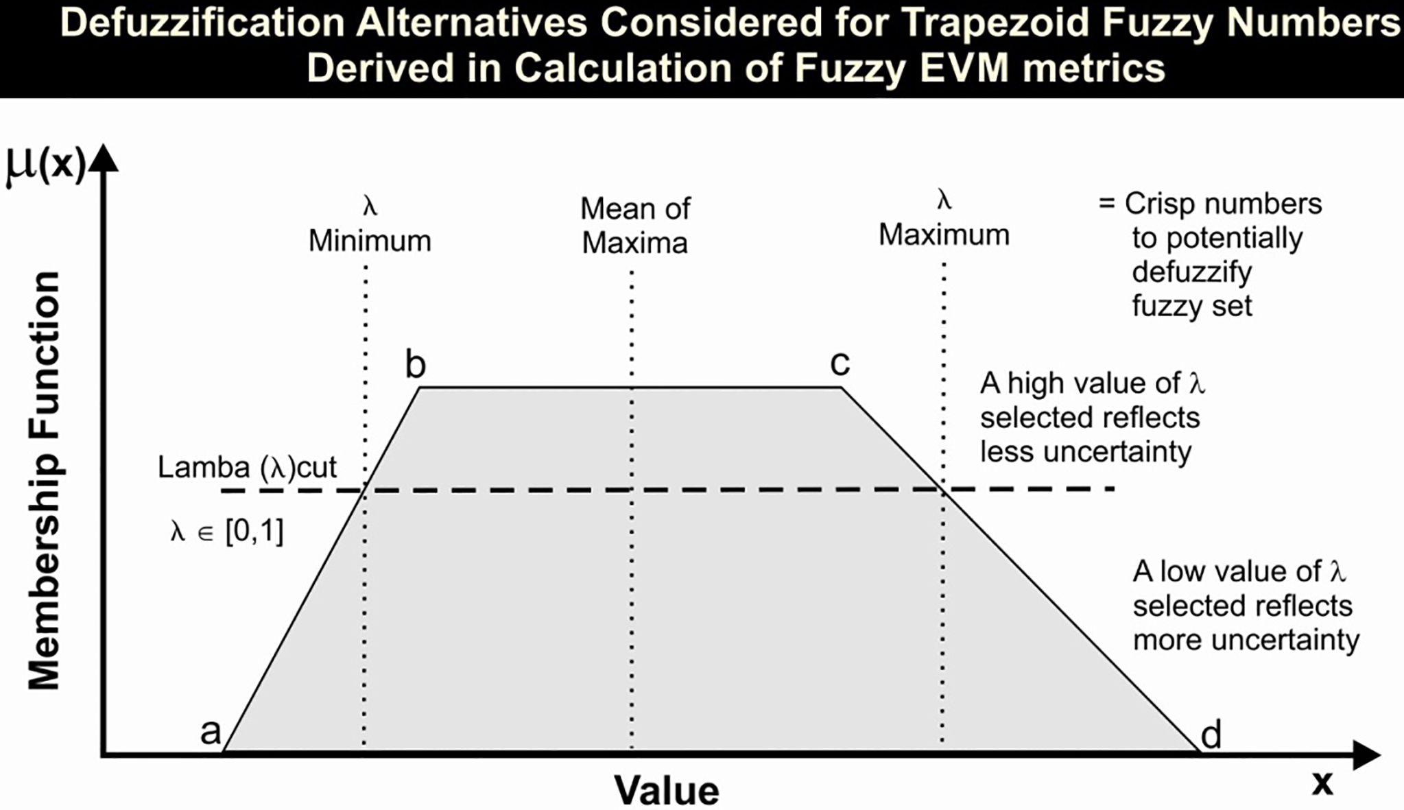$\lambda$ min-to- $\lambda$ max range can be quoted to indicate a possible range of associated uncertainty.

The trapezoidal fuzzy sets of fractions of work items completed lead to calculated fuzzy sets for ES, ED, EDcp, EDcpwt and derivative metrics yielding potential ranges for those metrics reflecting uncertainty in estimating work completed at any point along the BPS. In order to select a crisp number from the calculated fuzzy sets for each of these metrics three different defuzzification methods (Fig. 4) are applied (mean of maxima, minimum 50% lamba cut and maximum 50% lamba cut). Detailed analysis should include evaluating sensitivity cases using alternative lamba cut percentages.

Table 6 shows the crisp values of the ES, ED, EDcp and EDcpwt metrics and indices for the example project scenarios extracted from the fuzzy calculations using the minimum-50%-lamba-cut defuzzification calculation. These values are lower than those calculated by crisp deterministic and stochastic methods (Tables 3 and 4), but the maximum-50%-lamba-cut defuzzification calculation (Table 7) yields values much closer to the crisp stochastic methods using different input distribution types. Comparison of values in Table 6 with those in Tables 3 and 4 also indicates comparable relationships are achieved between ES, ED and EDcpwt calculated by crisp and fuzzy methods (i.e., EDcpwt yields more conservative values at the early stages of the BPS than ED or ES metrics). Table 6 shows that the unweighted-critical-path-only earned duration metric (EDcp) tends to over-estimate compared to ED and EDcpwt and is a less reliable indicator for the reasons already stated.

The selection of crisp numbers from the fuzzy sets can be calibrated with the values calculated by the non-fuzzy models by careful choice of the defuzzification method applied. For the example project, Table 7 reveals that the mean crisp values of ES, ED and EDcpwt extracted from the stochastic fuzzy models selected using the maximum-50%-lamba-cut method match quite closely with the mean values of the crisp stochastic models. This suggests that crisp simulation models run at the project planning stage could be used to calibrate fuzzy techniques to apply during project execution and select appropriate defuzzification methods and/or lamba cut percentages to apply.

Table 7 also demonstrates that the ranges displayed by the three alternative crisp numbers extracted from the fuzzy models generally represent between about 10% and 30% of the standard deviations calculated for the non-fuzzy stochastic models. This suggests that the fuzzy stochastic models are generally implying lower ranges of uncertainty than the non-fuzzy stochastic models represented in terms of a mean value plus or minus one standard deviation. Considering the $\lambda$ min-to- $\lambda$ max range of fuzzy ES, Ed and EDcpwt does provide some insight to the expected uncertainty associated with these metrics associated with the inability to determine exactly how much of each work item in progress has been completed at specific points along the BPS.

Table 6

Earned duration calculated values and indices for fuzzy and stochastic cases of example production plant construction project considered

Fuzzy case descriptions (best estimate case used as planned schedule and budget) defuzzification applying minimum Lamba cut of 50%	Fuzzy earned schedule (days)	Fuzzy schedule performance index (time based/cost derived)	Fuzzy SPIt- based projected project duration at completion (days)	Fuzzy earned duration (days)	Fuzzy duration performance index (time based/ time derived)	Fuzzy DPI- based projected project duration at completion (days)	Fuzzy earned duration critical path unweighted (days)	Fuzzy Duration performance index (time based from critical path)	Fuzzy DPIcpwt- based projected project duration at completion (days)	Fuzzy earned duration critical path weighted (days)	Fuzzy duration performance index (time based from critical path)	Fuzzy DPIcpwt- based projected project duration at completion (days)
Metric Abbreviation	ES	SPIt	PPDt	ED	DPI	PPDed	Edcp	DPIcp	PPDedcp	EDcpwt	DPIcpwt	PPDedcpwt
Best Estimate Case @20% of PD PD $=$ Planned Duration	178	0.958	910	176	0.945	918	216	1.159	744	170	0.911	923
Best Estimate Case @40% of PD	352	0.945	934	356	0.956	933	444	1.193	751	353	0.948	934
Best Estimate Case @60% of PD	525	0.940	941	532	0.954	935	554	0.992	909	519	0.930	935
Best Estimate Case @80% of PD	744	1.000	930	742	0.977	927	767	1.031	895	743	0.999	928
Best Estimate Case @100% of PD	930	1.000	930	930	1.000	930	930	1.000	930	930	1.000	930
Low Estimate Case @20% of PD	279	1.498	608	279	1.498	612	317	1.705	532	278	1.492	604
Low Estimate Case @40% of PD	525	1.410	624	528	1.419	633	554	1.489	606	519	1.395	624
Low Estimate Case @60% of PD	774	1.387	671	787	1.411	659	845	1.515	614	780	1.398	665
Low Estimate Case @80% of PD	930	1.250	670	930	1.250	670	930	1.250	670	930	1.250	670
Low Estimate Case @100% of PD	930	1.250	670	930	1.250	670	930	1.250	670	930	1.250	670
High Estimate Case @20% of PD	120	0.647	1394	135	0.725	1267	161	0.865	1039	121	0.650	1360
High Estimate Case @40% of PD	270	0.725	1242	272	0.732	1241	275	0.740	1191	248	0.665	1307
High Estimate Case @60% of PD	407	0.728	1238	407	0.728	1231	453	0.813	1116	388	0.695	1295
High Estimate Case @80% of PD	521	0.700	1258	529	0.711	1255	508	0.682	1323	495	0.665	1307
High Estimate Case @100% of PD	692	0.744	1236	694	0.746	1236	732	0.788	1169	702	0.754	1218
High Estimate Case @120% of PD	818	0.733	1225	818	0.733	1225	872	0.781	1170	823	0.737	1219
High Estimate Case @140% of PD	930	0.762	1220	930	0.762	1220	930	0.762	1220	930	0.762	1220

Table 7

Earned schedule and earned duration metrics calculations integrating fuzzy and stochastic analysis of example production plant construction project considered

Project progress duration monitoring
metrics, also used to provide reliable
forecasts of to-completion project											Earned duration critical path work items only
durations (l $=$ 0.5 for Lamba	Earned schedule – ES (Days)					Earned duration – ED (Days)					Weighted for planned work item
cut values shown)											durations – EDcpwt (Days)
Results of typical simulation run	Mean	Standard	Fuzzy	Fuzzy	Fuzzy	Mean	Standard	Fuzzy	Fuzzy	Fuzzy	Mean	Standard	Fuzzy	Fuzzy	Fuzzy
involving 1000 iterations.	stochastic	deviation	minimum	mean	maximum	stochastic	deviation	minimum	mean	maximum	stochastic	deviation	minimum	mean of	maximum
Lognormal and uniform inputs		stochastic	lamba cut	of	lamba cut		stochastic	lamba cut	of	lamba cut		stochastic	lamba cut	maxima	lamba cut
are used fo results shown,			(mean)	maxima	(mean)			(mean)	maxima	(mean)		(mean)	(mean)	(mean)
but similar estimate accuracies				(mean)					(mean)
are observed with other input
distribution formats
Lognormal distribution inputs:
Calculated Values @20% of PD	197	35.8	189	193	197	193	32.8	185	189	194	187	32.1	177	182	188
Calculated Values @40% of PD	382	47.7	371	376	381	383	47.5	373	378	383	380	47.9	369	374	379
Calculated Values @60% of PD	561	54.2	543	552	561	559	54.6	546	553	559	560	53.9	540	551	561
Calculated Values @80% of PD	741	64.2	731	736	741	743	63.6	734	739	743	739	66.1	729	734	739
Calculated Values @100% of PD	900	44.4	891	896	901	900	44.0	891	896	901	900	44.5	891	896	901
Uniform distribution inputs:
Calculated Values @20% of PD	190	43.7	182	186	190	189	40.7	180	185	188	182	37.2	172	177	182
Calculated Values @40% of PD	371	57.8	360	365	370	372	57.9	362	366	371	367	56.8	356	361	367
Calculated Values @60% of PD	546	64.3	527	537	546	546	64.3	530	538	545	545	63.6	524	535	545
Calculated Values @80% of PD	724	77.4	713	718	723	726	76.7	716	721	726	720	79.5	709	715	720
Calculated Values @100% of PD	881	58.4	870	876	881	881	57.8	870	876	882	880	58.7	869	875	881

Comparison of the results of the deterministic, fuzzy and crisp stochastic models applied to the example project suggest that EDcpwt provides valuable, more-sensitive and complementary performance-monitoring information to the analysis provided by ES and ED metrics and it is a worthwhile metric to calculate.

3.4 To-completion forecasts for example project applying ES and ED metrics

Although the deterministic and stochastic models can be configured to calculate a large number of metrics related to EV, ES and ED derivative indices that facilitate to-completion forecasts of project cost and duration, the challenge is often to decide which metrics are the most reliable for a specific project. Percentage errors on mean stochastic values associated with to-completion predictions versus actual completion values for each specific scenario evaluated at various points along the BPS based on the simulation trials provide useful insight (Table 8). Comparison of such errors helps to establish the reliability of the to-completion predictions for a given set of input assumptions. Table 8 compares the percentage errors on the mean values associated with several to-completion forecast metrics at specified points along the BPS for simulation runs with lognormal and uniform input distributions. The errors generally are higher for the earlier-stage estimates (i.e., 20%PD and 40%PD) and lower for later stage estimates (i.e., 60%PD and 80%PD), as there is less uncertainty in the durations of work items remaining to be completed for the late stage estimates. Bear in mind that at 100%PD many simulation scenarios still have significant work items left to be completed (i.e., those scenarios that involve delays to critical path and/or crucial work items).

For the example project, early-stage forecasts of to-complete project costs based on the widely-used PAC metric (CPI-derived) result in percentage error on distribution mean values in the range of 5% to 10%. These errors fall to below 1% for later stage estimates for that metric. For the to-completion duration forecasts, the PPD metric (SPI-derived) forecasts are the least reliable for the example project data set, involving high errors associated, in particular, with the early-stage forecasts (Table 8). On the other hand, the PPDt, PPDed, PPDcp and PPDcpwt metrics provide much more reliable forecasts, with errors in the 1% range for forecasts made at 40%PD and later rising only slightly for the 20%PD forecasts. The PPDt (earned-schedule-derived) is rightly widely used for such estimates. However, it makes sense to also monitor PPDed (earned-duration-derived) and PPDcpwt forecasts to provide additional insight.

Another useful error measure for to-completion estimates associated with each scenario evaluated in a simulation is the mean absolute percentage error (MAPE). The MAPE errors associated with various projected project durations (PPD) calculated by crisp and fuzzy simulations using lognormal and uniform input distributions are compared in Table 9. PPDt, PPDed and PPDedcpwt forecasts show low and comparable MAPE values of less than about 3% for earlier-stage forecasts (@20%PD), falling to less than 1% for later-stage forecasts (>@60%PD). The @20%PD and @40%PD forecasts for PPDedcpwt demonstrate slightly higher MAPE values than PPDed and PPDt, due to their greater sensitivity to delays in early-stage and crucial work items. MAPE values for the PPDedcp to-completion forecasts (i.e. unweighted) are much higher than for the other forecasts (e.g., close to 20% for @20%PD estimates) demonstrating its unreliability as a forecasting metric. As to be expected, the MAPE values for the later-stage-to-completion forecasts (>@60%PD) are lowest for stochastic models with input data sampled as lognormal distributions and highest for those sampled with uniform distributions. Both distribution types evaluated confirm the reliability of the PPDt, PPDed and PPDedcpwt forecasting metrics for the example project.

Table 8
To-completion forecast errors for cost and duration based upon stochastic analysis of example production plant construction project considered

	Cost at completion		Project duration to-completion forecasts
	estimates: differences		differences to actual duration at completion
	to actual costs
Metrics from which to-	Estimates derived		Estimates derived		Estimates derived		Estimates derived		Estimates derived		Estimates derived
completion estimates	from CPI		from SPI		schedule (SPIt)		duration		critical path (weighted)		critical path (not weighted)
are derived	from CPI				schedule (SPIt)		duration		critical path (weighted)		critical path (not weighted)

Results of typical simulation run involving 1000 iterations. Lognormal and uniform Inputs are used for results shown, but similar estimate accuracies are observed with other input distribution formats	Mean PAC-ACaC ($ millions)	Mean PAC-ACaC as % of ACaC
(Days)	Mean PPD-ADaC as % of ADaC		Mean PPD-ADaC
(Days)	Mean PPDt-ADaC as % of ADaC	Mean PPDt-ADaC
(Days)	Mean PPDed-ADaC as % of ADaC	Mean PPDcpwt-ADaC (Days)	Mean PPDcpwt-ADaC as % of ADaC	Mean PPDcp-ADaC (Days)	Mean PPDcp-ADaC as % of ADaC
Lognormal distribution inputs:
To Completion Estimates @20% of PD	55.35	5.56%	341.42	36.49%	$-$ 26.25	$-$ 2.81%	$-$ 17.08	$-$ 1.83%	$-$ 13.57	$-$ 1.45%	$-$ 5.22	$-$ 0.56%
To Completion Estimates @40% of PD	25.07	2.52%	$-$ 28.50	$-$ 3.05%	$-$ 8.77	$-$ 0.94%	$-$ 11.98	$-$ 1.28%	$-$ 13.63	$-$ 1.46%	$-$ 11.75	$-$ 1.26%
To Completion Estimates @60% of PD	9.52	0.96%	9.38	1.00%	4.13	0.44%	5.89	0.63%	$-$ 10.97	$-$ 1.17%	5.11	0.55%
To Completion Estimates @80% of PD	$-$ 1.36	$-$ 0.14%	26.18	2.80%	7.00	0.75%	4.33	0.46%	6.36	0.68%	7.64	0.82%
To Completion Estimates @100% of PD	$-$ 0.33	$-$ 0.03%	$-$ 23.70	$-$ 2.53%	2.62	0.28%	2.47	0.26%	1.47	0.16%	2.48	0.26%
Uniform distribution inputs:
To Completion Estimates @20% of PD	108.09	10.66%	722.09	74.99%	7.80	0.81%	3.72	0.39%	$-$ 4.92	$-$ 0.51%	11.66	1.21%
To Completion Estimates @40% of PD	58.23	5.74%	$-$ 25.55	$-$ 2.65%	2.54	0.26%	$-$ 0.26	$-$ 0.03%	$-$ 5.77	$-$ 0.60%	$-$ 0.02	0.00%
To Completion Estimates @60% of PD	19.95	1.97%	72.91	7.57%	8.92	0.93%	10.59	1.10%	$-$ 9.04	$-$ 0.94%	8.80	0.91%
To Completion Estimates @80% of PD	$-$ 1.65	$-$ 0.16%	50.85	5.28%	14.44	1.50%	10.91	1.13%	8.20	0.85%	17.05	1.77%
To Completion Estimates @100% of PD	$-$ 1.22	$-$ 0.12%	$-$ 42.67	$-$ 4.43%	6.01	0.62%	5.49	0.57%	4.21	0.44%	5.56	0.58%

Table 9

To-completion duration forecast mean absolute percentage errors from stochastic analysis of crisp and fuzzy simulation models for example production plant construction project considered

Project duration to-completion forecasts: Percentage differences to actual duration at completion for each simulation case evaluated
Metrics from which to completion	MAPE PPDt		MAPE PPDed		MAPE PPDedcpwt		MAPE PPDedcp
estimates are derived	(% of ADaC)		(% of ADaC)		(% of ADaC) weighted		(of ADaC) unweighted
	(% of ADaC)		(% of ADaC)		(% of ADaC) weighted		(of ADaC) unweighted
Results of typical simulation run involving	Crisp	Fuzzy (min	Crisp	Fuzzy (min	Crisp	Fuzzy (min	Crisp	Fuzzy (min
1000 iterations. Lognormal and uniform Inputs are used for results shown, but similar estimate accuracies are observed with other input distribution formats	stochastic	Lamba cut)	stochastic	Lamba cut)	stochastic	Lamba cut)	stochastic	Lamba cut)
Lognormal distribution inputs:
To Completion Estimates @20% of PD	1.91%	2.17%	0.93%	1.10%	$-$ 1.55%	$-$ 1.54%	19.22%	19.28%
To Completion Estimates @40% of PD	1.04%	0.81%	1.34%	1.18%	0.50%	0.28%	18.88%	18.83%
To Completion Estimates @60% of PD	$-$ 0.24%	$-$ 0.25%	$-$ 0.47%	$-$ 0.56%	$-$ 0.40%	$-$ 0.29%	3.80%	3.83%
To Completion Estimates @80% of PD	$-$ 0.60%	$-$ 0.68%	$-$ 0.31%	$-$ 0.33%	$-$ 0.88%	$-$ 0.94%	3.56%	3.53%
To Completion Estimates @100% of PD	$-$ 0.25%	$-$ 0.23%	$-$ 0.23%	$-$ 0.25%	$-$ 0.26%	$-$ 0.29%	1.20%	1.16%
Uniform distribution inputs:
To Completion Estimates @20% of PD	$-$ 0.47%	$-$ 0.66%	$-$ 0.42%	$-$ 0.46%	$-$ 3.24%	$-$ 3.53%	19.40%	19.27%
To Completion Estimates @40% of PD	0.08%	$-$ 0.07%	0.31%	0.20%	$-$ 0.82%	$-$ 0.95%	17.43%	17.41%
To Completion Estimates @60% of PD	$-$ 0.64%	$-$ 0.71%	$-$ 0.79%	$-$ 0.92%	$-$ 0.96%	$-$ 0.94%	4.77%	4.78%
To Completion Estimates @80% of PD	$-$ 1.09%	$-$ 1.14%	$-$ 0.78%	$-$ 0.79%	$-$ 1.59%	$-$ 1.62%	2.42%	2.40%
To Completion Estimates @100% of PD	$-$ 0.56%	$-$ 0.55%	$-$ 0.51%	$-$ 0.53%	$-$ 0.60%	$-$ 0.64%	1.58%	1.54%

3.5 Establishing confidence levels in specified budget and duration targets

Although ES, ED and EDcpwt are useful project monitoring and to-completion forecasting metrics they do not provide sufficient insight to much of the uncertainty associated with typical projects. Just because a project has performed at a certain level up to a specific point along the BPS, it does not mean that it will continue to do so. Work items yet to start may be delayed for all sorts of unforeseen reasons. Applying fuzzy techniques is able to capture some of the future uncertainty that is essentially ignored by EV, ES and ED metrics. However, unlike probabilistic methods, fuzzy methods do not provide sufficient information to establish meaningful confidence levels associated with achieving specified targets. For most projects it is useful to be able to evaluate the probability of achieving the budget and schedule targets set, and stochastic models calculating probabilistic downside risk measures are required to provide this.

Table 10 provides three stochastic measures of downside risk (i.e. the risk of failing to achieve specified values) for a range of schedule and budget targets associated with the example project. These are: 1) the number of scenarios sampled in a simulation that yields values above a specified target (which says nothing about the magnitudes by which the targets are breached); 2) mean values of scenarios breaching a target; 3) the semi-standard deviation (SSD-see appendix for calculation formula) of scenarios breaching a target. The latter two downside risk measures express that risk quantitatively in the units of the target. The semi-standard deviation (SSD) downside-risk measure [31] can also be used to establish appropriate contingencies to apply when setting targets.

Table 10
Evaluation of project duration at-completion targets of example production plant construction project considered

Based upon 1000 trial stochastic analysis based upon stochastic analysis
Project	Number of 1000	Mean of the values	Semi-standard
durationtargets	trials run	above target	deviation (SSD)
tested (days)	above target	(days)	above target (days)
800	973	938	151.2
830	932	943	125.2
860	863	951	100.8
890	736	964	78.7
920	546	985	59.3
950	391	1005	42.8
980	263	1025	29.2
1010	150	1048	18.7
1040	77	1070	10.9
1070	30	1095	5.8

Figure 5.

Example-project stochastically-derived downside risk comparisons of a range of at-completion duration targets for the example project. The downside risks are quantified in day units using the semi-standard deviation (SSD) measure.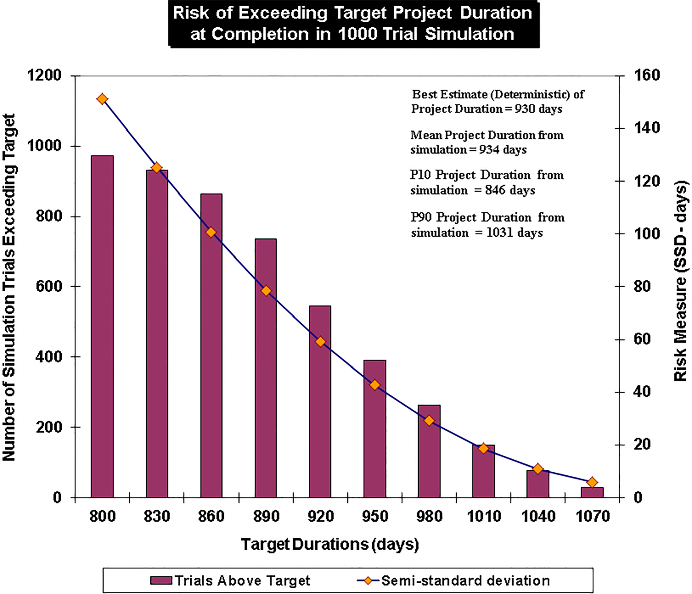

Table 10 and Fig. 5 demonstrate the usefulness of downside risk measures, particularly SSD, in establishing the confidence of achieving at-completion project duration targets. The at-completion project duration analysis (Fig. 5) indicates that targets below about 920 days are at high-risk of being breached, with greater than 50% of the simulation trials failing to complete the project within those targets and SSD values of greater than 50 days.

The earned-value-derived to-complete cost performance index (TCPI) and earned-schedule-derived to-complete schedule performance index (TSPI) [14] can provide some insight regarding the likelihood of targets being met. Values of TSPI and TCPI below “1” imply that a project is able to achieve the targets tested. On the other hand, values of TSPI and TCPI above “1.1” imply that a project is unlikely to achieve the specified target [18]. The TSPI indicator could be calculated using DPI or DPIcpwt metrics in addition to SPI or SPIt metrics. However, the TSPI and TCPI metrics do not provide confidence levels associated with such targets, which are more meaningfully provided by stochastic analysis.

Stochastic models can also establish the “criticality” of a work-item or work-item-pathway for the scenarios sampled. Criticality is the probability that a work item is situated on the critical path. The critical path can shift between work item pathways depending upon the work item duration assumptions applied. Once the criticality of work items is known project resources can be concentrated on those work items with high levels of criticality. The importance of work item criticality/cruciality and the confidence levels of achieving targets justify developing stochastic models for project cost-time evaluation that focus on a range of uncertainties in addition to the earned value, schedule and duration metrics. Weighting earned duration, with the planned duration of each work item relative to all work items along the critical path, incorporates work-item cruciality into earned duration analysis and thereby can enhance stochastic models.

4. Conclusions

When conducting duration and schedule analysis of project networks there is justification to calculate earned duration metrics in three different ways, for project performance monitoring and to-completion forecasting, for the following reasons:

ED and DPI are calculated incorporating all project work item durations to compare with earned schedule (ES) metrics (derived as part of established earned value management). The comparison can be used to test whether the assumption that cost progress and duration progress towards completion is highly-positively correlated.

EDcp and DPIcp focus just upon critical path items thereby removing potential biases in projects with multiple pathways. This metric can potentially compensate for instances where non-critical items performed quicker than planned can obscure delays in critical path items resulting in ED and ES providing over-optimistic indications of performance.

EDcpwt and DPIcpwt monitor critical-path work items taking into account the magnitude of planned duration of each work item. This metric can overcome the potential for a number of shorter duration work items being completed, but slower than planned, yet still resulting EDcp and ED failing to penalize performance indications sufficiently enough for delaying crucial, long-duration work items yet to be started.

Comparisons of ED and EDcpwt metrics with ES metrics for an example project analysis suggest that these metrics provide complementary information and can collectively be used to provide more reliable project monitoring and to-completion forecasting in deterministic, stochastic and fuzzy network analysis models. The EDcp metric is less reliable than the other measures as it can be distorted by the relative performance of work items of significantly different durations. Calculated in a deterministic way, all EV, ES and ED metrics and derivative indices fail to adequately take account of project uncertainties. Stochastic and fuzzy methods do take more account of uncertainty, and stochastic models are able to compute additional probabilistic downside risk measures that provide confidence levels on certain targets being met. This justifies conducting fuzzy and stochastic risk analysis to enhance deterministic EV, ES, ED and EDcpwt analysis. Of course, for relatively simple project networks without multiple parallel pathways of work items making these additional calculations would not be necessary, and a simpler approach would reduce computation time.

Footnotes

Appendix 1: Abbreviations for EVM-related metrics

The following, in alphabetical order, lists the abbreviations/acronyms used in this manuscript. Calculation formulas are included for some of the metrics.

AD Actual Duration

ADaC Actual Project Duration at (Project) Completion

APC Actual Percentage (of project) Completed

APCt Actual Percentage (of project) Completed at specified time (t)

APCtcp Actual Percentage (of project’s critical path work items) Completed at time (t)

APCtcpwt Actual Percentage (of project’s critical path work items) Completed at time (t) with the calculation weighted for planned durations of each critical-path work item

BaC Budget at Completion

BPS Baseline Planned Schedule (sometimes referred to as a project’s “makespan”)

CPI Cost Performance Index [EV/AC]

CR Project Criticality Index [CPI * SPI] sometimes called CSI Cost Schedule Index (SPI is typically replaced with SPIt based upon more reliable ES measure of schedule performance)

CRcp Project Criticality Index critical path [CPI * DPIcp]

CRcpwt Project Criticality Index critical path weighted [CPI * DPIcpwt]

CSPF Cost Schedule Performance Factor (see note 1)

CSPFcp Cost Schedule Performance Factor (involving DPIcp; see note 1)

CSPFcpwt Cost Schedule Performance Factor (involving DPIcpwt; see note 1)

Di Duration of work item i (i is an individual work item or activity)

Dipcp planned duration of critical path work item i

DPI Duration Performance Index (DPIx is DPI at time point x)

DPIcp Duration Performance Index calculated for critical path work items only

DPIcpwt applying weighted average work item durations to adjust the DPIcp calculation

ED Earned Duration (see note 2)

EDcp Earned Duration calculated for critical path work flow items only (see note 2)

EDcpwt Earned Duration calculated for critical path work flow items only with work-flow-durations weighting applied to take account of crucial work flows

EDaC Estimated Duration at Completion

EF Earliest Finish (for individual work item or activity)

ES Earned Schedule (see note 2)

ESt Earliest Start (for individual work item or activity)

EV Earned Value

EVM Earned Value Management

$f_{i}$ is the fraction of work item “i” that is completed

$f_{icp}$ is the fraction of critical path work item “i” that is completed

F Float (sometimes referred to as slack) is the amount of time that a work flow item or activity can be delayed without causing a delay to either subsequent tasks (“free float”) or the project completion date (“total float”)

LF Latest Finish (for individual work item or activity)

LSt Latest Start (for individual work item or activity)

PD Planned Duration (of project at completion); sometimes referred to as the project’s makespan

PDt Planned Duration at a specific time (t) along the baseline planned schedule or makespan

PPC Planned Percentage (of project) Completed

PPCcp Planned Percentage (of project) Completed based upon critical-path work items only

PPCcpwt Planned Percentage (of project) Completed based upon critical-path work items only weighted for planned durations of the critical-path work items

PPCt Planned Percentage (of project) Completed at specified time (t)

PPD Projected Project Duration (at Completion) [PD/SPI] EV-based calculation

PPDt Projected Project Duration (at Completion) [PD/SPIt] ES-based calculation

PPDed Projected Project Duration (at Completion) [PD/DPI] ED-based calculation

PPDedcpwt Projected Project Duration (at Completion) [PD/DPIcpwt] ED critical path-based calculation

PV Planned Value

PVt Planned Value at a specific time (t) along the planned schedule

SPI Schedule Performance Index [EV/PV]

SPIt Earned Schedule, Schedule Performance Index [ES/AD]

SSD Semi-standard Deviation (downside risk statistic calculated with reference to a specified target) (see note 2)

TCPI To-completion Cost Performance Index [(BaC-EV)/(Target-AC)] (Target could be budget at completion or another relevant project cost objective, e.g., BaC plus contingency)

TSPI To-completion Schedule Performance Index [(PD-ES)/(Target-AD)] (Target could be planned duration or another relevant project schedule objective, e.g., PD plus contingency)

WBPD Work Breakdown Progress Diagram

WBS Work Breakdown Structure

Wtot Sum of all work-item (or activity) durations ignoring parallel execution pathways

Notes:

(1)

Cost Schedule Performance Factor [4] is calculated with the formula:

$=$ $+$ $-$ $+$

where: Fa $=$ 1/CPI and Fs $=$ 1/SPI

Values of CSPF at any point (t) along the planned duration indicate that the project is either behind schedule or overrunning its budget. Modified CSPF using Fs $=$ 1/SPIt or Fs $=$ DPI instead of SPI improve the reliability of the index.

(2)

SSD semi-standard deviation is a useful statistic to quantify downside risk relative to a target value in the units of the metric being assess. It is calculated using the formula:

$\text{SSD}=\surd\frac{1}{N}\mathop{\sum}\limits_{v<t}(v-t)^{2}$

where: “ $t$ ” is the target value ; “ $v$ ” is any value in the distribution with a value less than target value “ $t$ ”; and, “ $N$ ” is the total number of values in the distribution above target value “ $t$ ”. It is analogous to a standard deviation but focused just on samples that fall within the downside portion of a distribution. Wood [31] showed how this measure could be used effectively to measure downside risk of project cost and time targets.

Appendix 2: Calculation methods

Deterministic models are those in which no randomness is involved in its elements. In the context of this work this means that estimates of each work item’s costs and durations are fixed at the planning stage with no possibility for variation in the model’s execution. Much current theory and practice associated with earned value management and earned schedule calculations assumes deterministic project networks. Deterministic models are useful for verifying project network logic and for setting planned project budgets and schedules, but need to be complemented by stochastic and/or fuzzy models in order to give due consideration to the uncertainties associated with most work item’s costs and durations (for those work items yet-to-be completed).

Stochastic models incorporate uncertainty associated with input assumptions (in the current work that is project work item costs and durations), and sample those uncertain inputs randomly in order to calculate probability distributions of key outputs (i.e., in the current work that is total project duration and total project cost at project completion and the amount of time and cost yet to be incurred by outstanding work items). Three key uncertain input variables are included in the stochastic models developed here. They are work item duration, semi-fixed and variable work item costs, which may vary independently of each other or be correlated in with each other in some way either positively or negatively. The uncertainties associated the output distributions from stochastic models are usefully expressed in statistical terms, i.e., means, percentiles, levels of confidence, variances and standard deviations.

Fuzzy models involve fuzzy logic and fuzzy set theory, first defined and exploited in its modern context by Zadeh [33]. Whereas classic logic only permits binary type assessments (e.g., true or false), fuzzy logic acknowledges grades of partial knowledge, subjectivity or perception/vagueness. Probabilistic/ stochastic models apply a mathematical model using the scale of 0 (something will never occur) to 1 (something will occur with certainty, and grades in between. On the other hand, fuzzy logic uses degrees of truth or knowledge as a mathematical scale, also typically expressed on a scale of 0 to 1, of vagueness. Fuzzy logic enables linguistic assessments of the status of an uncertain input variables to be translated, via membership functions, into a degree of membership. Where available information is vague or assessments are subjectively made with limited access to detailed information, fuzzy models often work better than probabilistic models, or can at least complement them. In the context of the current work, the subjective assessment made by project operators of the degree of work completed, often in vague linguistic terms, of work items currently in progress is well suited to being treated via fuzzy logic and assessed as part of a fuzzy model. It is this aspect of project duration uncertainty that is explored by fuzzy models in this study.

References

Acebes

Pereda

Poza

Pajares

and Galán

J.M.

, Stochastic earned value analysis using Monte Carlo simulation and statistical learning techniques, International Journal of Project Management 33 (2015), 1597–1609.

Anbari

F.T.

, Earned value project management method and extensions, Proj. Manag. J. 34(4) (2003), 12–23.

Batselier

and Vanhoucke

, Evaluation of deterministic state-of-the-art forecasting approaches for project duration based on earned value management, International Journal of Project Management 33 (2015), 1588–1596.

Cioffi

D.F.

, Designing project management: a scientific notation and an improved formalism for earned value calculations, International Journal of Project Management 24(2) (2006), 136–144.

Fleming

Q.W.

and Koppelman

J.M.

, The Essence of Evolution of Earned Value, Cost Engineering 36(11) (1994), 21–27.

Hazir

Ö.

, A review of analytical models, approaches and decision support tools in project monitoring and control, International Journal of Project Management 33(4) (2015), 808–815.

Henderson

, Earned schedule: a breakthrough extension to earned value theory? The Measurable News (Summer 2003), 13–23.

Jacob

D.S.

, Is “Earned Schedule” an unreliable indicator? No, but It’s not necessarily the premier indicator for assessing schedule performance, The Measurable News 6 (2006).

Jacob

D.S.

and Kane

, Forecasting schedule completion using earned value metrics…revisited, The Measurable News (2004), 10–17.

10.

Khamooshi

and Golafshani

, EDM: Earned Duration Management, a new approach to schedule performance management and measurement, International Journal of Project Management 32 (2014), 1019–1041.

11.

Kim

E.-H.

Wells

W.G.

and Duffey

M.R.

, A model for effective implementation of Earned Value Management methodology, International Journal of Project Management 21 (2003), 375–382.

12.

Lipke

, Schedule is different, The Measurable News 3 (2003), 31–34.

13.

Lipke

, Applying Earned Schedule to Critical Path Analysis and More’, The Measurable News Fall Edition (2006), 26–30.

14.

Lipke

, The To Complete Performance Index …an expanded view, The Measurable News (2) (2009), 18–22.

15.

Lipke

Zwikael

Henderson

and Anbari

, Prediction of project outcome: the application of statistical methods to earned value management and earned schedule performance indexes, International Journal of Project Management 27(4) (2009), 400–407.

16.

Lipke

, Speculations on Project Duration Forecasting, The Measurable News 3(1) (2012), 4–7.

17.

Lipke

, Applying statistical forecasting of project duration to earned schedule-longest path, PM World Journal IV(II) (2015), 1–13.

18.

Lipke

, The To Complete Performance Index …an expanded view, The Measurable News (2) (2016), 18–22.

19.

Lukas

J.A.

, Earned Value Analysis – Why it Doesn’t Work, AACE International Transactions EVM (1) (2008), 1–10.

20.

Mowery

, Earned schedule: from emerging practice to practical application, Computer Sciences Corporation, Leading Edge Forum, 2012, 28. http://assets1.csc.com/innovation/downloads/CSC_Papers_2012_Earned_Schedule.pdf.

21.

Naeni

L.M.

and Salehipour

, Evaluating fuzzy earned value indices and estimates by applying alpha cuts, Expert Syst. Appl. 38(7) (2011), 8193–8198.

22.

Naeni

L.M.

Shadrokh

and Salehipour

, A fuzzy approach for the earned value management (Erratum), International Journal of Project Management 32 (2014), 709–717.

23.

Noori

Bagherpour

and Zareei

, A. Applying Fuzzy Control Chart in Earned Value Analysis: A New Application, World Applied Sciences Journal 3(4) (2008), 684–690.

24.

Project Management Institute, Practice Standard for Earned Value, Management Newtown Square, PA, Project Management Institute, 2005.

25.

Project Management Institute, 2013. A guide to the project management body of knowledge (PMBOK Guide) Fifth Edition, Project Management Institute (2013), 589 pages.

26.

Soroush

H.M.

, The most critical path in a PERT network, The Journal of Operational Research Society 45(3) (1994), 287–300.

27.

Vandevoorde

and Vanhoucke

, A comparison of different project duration forecasting methods using earned value metrics, International Journal of Project Management 24(4) (2006), 289–302.

28.

Vandevoorde

and Vanhoucke

, A simulation and evaluation of earned value metrics to forecast the project duration, Journal of the Operational Research Society 58 (2007), 1361–1374.

29.

Vanhoucke

, Measuring the efficiency of project control using fictitious and empirical project data, International Journal of Project Management 30 (2012), 252–263.

30.

Williams

T.M.

, Criticality in stochastic networks, Journal of Operational Research Society 43 (1992), 353–357.

31.

Wood

D.A.

, Probabilistic methods with simulation help predict timing, cost of projects, Oil & Gas Journal (12 Nov 2001), 79–83.

32.

Wood

D.A.

, Gas and Oil Project Time-Cost-Quality Tradeoff: Integrated Stochastic and Fuzzy Multi-Objective Optimization Applying a Memetic, Nondominated, Sorting Algorithm, Journal of Natural Gas Science and Engineering 45 (2017), 143–164.

33.

Zadeh

L.A.

, Fuzzy sets, Information and Control 8(3) (1965), 338–353.

A critical-path focus for earned duration increases its sensitivity for project-duration monitoring and forecasting in deterministic,fuzzy and stochastic network analysis

Abstract

Keywords

1. Introduction

2. Earned duration: Justifications for alternative computations

2.1 Potential drawback associated with Earned schedule (ES)

3.1 Description of example project in terms of duration and schedule

Table 1 Network logic for example production plant construction project work items

Table 2 Deterministic case and planned schedule outcomes for example production plant construction project considered

Table 5 Uncertain work item progress towards completion ne expressed as a trapezoidal fuzzy Set-X[a,b,c,d]

Table 8 To-completion forecast errors for cost and duration based upon stochastic analysis of example production plant construction project considered

Table 10 Evaluation of project duration at-completion targets of example production plant construction project considered

Footnotes

Appendix 1: Abbreviations for EVM-related metrics

Appendix 2: Calculation methods

References

Table 1
Network logic for example production plant construction project work items

Table 2
Deterministic case and planned schedule outcomes for example production plant construction project considered

Table 5
Uncertain work item progress towards completion ne expressed as a trapezoidal fuzzy Set-X[a,b,c,d]

Table 8
To-completion forecast errors for cost and duration based upon stochastic analysis of example production plant construction project considered

Table 10
Evaluation of project duration at-completion targets of example production plant construction project considered