Theoretical studies of combustion have mostly focused on low speed deflagrations as well as pure supersonic detonations; however, transonic conditions, have not been as widely studied. Transonic flow conditions naturally occur in a variety of applications such as: turbine engines, power generation systems, missiles, turbo-machinery, industrial reactors and many more. A small disturbance and irrotational model is proposed in [11]. The current work investigates relaxing the small disturbance assumption. In addition, the common practice is to treat the pressure equation as elliptic (pressure correction methods, pressure projection methods). Instead, a hyperbolic equation for the pressure is used in this study for unsteady problems. The current work investigates integration of the hyperbolic pressure equation as part of a reactive full potential flow model.
Increasingly computer simulations are being used in engineering, and simulations involving the reactive Euler equations are expensive and simplified models can reduce the calculations a design team needs to do. For this reason small disturbance, or potential models, which may be permissible under certain operating conditions are desirable. Rusak et al. demonstrated that steady state solutions of the compressible reacting flow problem with detonations behind the shock waves can be found. The model was used to study transonic combustion at various inlet Mach numbers, amounts of incoming reactant mass, reaction rates, and channel geometries [11]. The present work has two principal goals: (1) to extend the small disturbance combustion model proposed in [11] for transonic full potential flows, and (2) to develop a pressure-based unsteady Euler model that is capable of handling the effect of chemical reactions. Thus, in the present work we investigate a natural alternative model that fits between a reactive small disturbance model and a full reactive Euler model.
Combustion equations
The general governing equations, including viscous effects, are the two-dimensional compressible reactive flow Equations for a premixed chemical fuel species with Arrhenius type kinetics:
Where is the viscosity, is the thermal conductivity, is the pre-exponential reaction factor, and is the diffusivity coefficient, is the viscous dissipation and is the mass diffusion, and is the specific heat release. The choice of premixed chemistry with Arrhenius kinetics is to emphasize the effect of heat release with realistic reaction rates coupled to the flow. is a reaction progress variable, , where means the reactant is fully consumed, and implies no reaction has yet taken place.
Nondimensionalization
Consider a compressible flow of a reactive fluid in a two dimensional channel. Letting the -state denote the uniform flow conditions at the channel inlet, a non-dimensionalization is made by, where denotes a dimensional variable, the inlet condition and L is half the width of the channel:
Some authors non-dimensionalize , a conversion between this non-dimensionalization and ours is given by:
The dimensionless parameters are given by:
Now, the dimensionless governing equations, in the inviscid limit of the momentum equations, without viscous dissipation or mass diffusion become:
Where is the Prandtl Number, and is the Schmidt Number. This is a model for the reactive Euler Equations for compressible flow with premixed Arrhenius combustion, see [1, 7] for more details.
Reactive transonic full potential model
Decomposition of the velocity field into a curl-free component and a divergence-free component gives:
This Helmholtz orthogonal decomposition of the velocity field gives us a potential and stream function formulation for the compressible Euler Eq. (2.1) without combustion ( 0):
Where and stand for the inertia terms in the momentum equations. The above Poisson equation for the pressure is derived by taking the divergence of the momentum equations in primitive variables:
This model admits the incompressible flow solution as a special case when density is constant. Some simplifications of the above model are possible. For example, in the case of irrotational compressible flow, the stream function equation can be omitted, and in the case of irrotational incompressible flow, instead of the pressure equation, Bernoulli’s law can be used. We will assume the flow is irrotational (i.e. ), but we will account for heat release due to chemical reaction coupling as in the reactive Euler Equations. In particular, for the expanding duct flow under consideration in this paper, shock fronts are almost normal to the principal flow direction. Since Crocco relation relates vorticity to shock curvature [8], this suggests a framework where under such conditions a compressible potential flow model might be used.
For irrotational flows, a velocity potential function must exist such that . Under this assumption the velocity field is curl-free and reduces to: , . An irrotational unsteady compressible reactive full potential flow model is given by:
It should be noted that unlike the classical density-based approach, this is a pressure-based approach. For steady flow, the pressure equation can be treated as a Poisson’s equation. For unsteady flow, the following hyperbolic equation for pressure is introduced:
For the present work we simply choose:
Reactive transonic small disturbance model
Using a small disturbance expansion around uniform inlet conditions gives a reactive transonic small disturbance model similar to that proposed in [11]:
This governing equation is of mixed type, elliptic and hyperbolic. Here denote small disturbance variables, and and are constant reaction control parameters, and is the inlet Mach number. The velocity can be calculated from: . Details of the derivation, scaling, and variations are available in [11]. The small disturbance approach is limited to small heat release, i.e. diluted premixtures, and small area variation. According to [11] the precise limitations are upstream flows with Mach number between 0.75 and 1.2, premixtures with reactant mass fractions up to 0.1, and channel cross-sectional area variation of 15 percent or less. The boundary conditions at the channel inlet () are:
where . We will take in this work. At the channel outlet ():
Small Disturbance Model (TSD) for 0.75, 0.80, 0.85, 0.90, 0.95 for 0, showing transition to shocked flow with Zeirup Singularity at 12% nozzle area variation parameter.
Small Disturbance Model (TSD) T and Y profiles for 0.75 for 0, 10000, 20000, 30000. Higher pre-exponential frequency factor consumes more reactant (left), results in a lower thermal energy (middle) and higher Mach number (right) at the outlet.
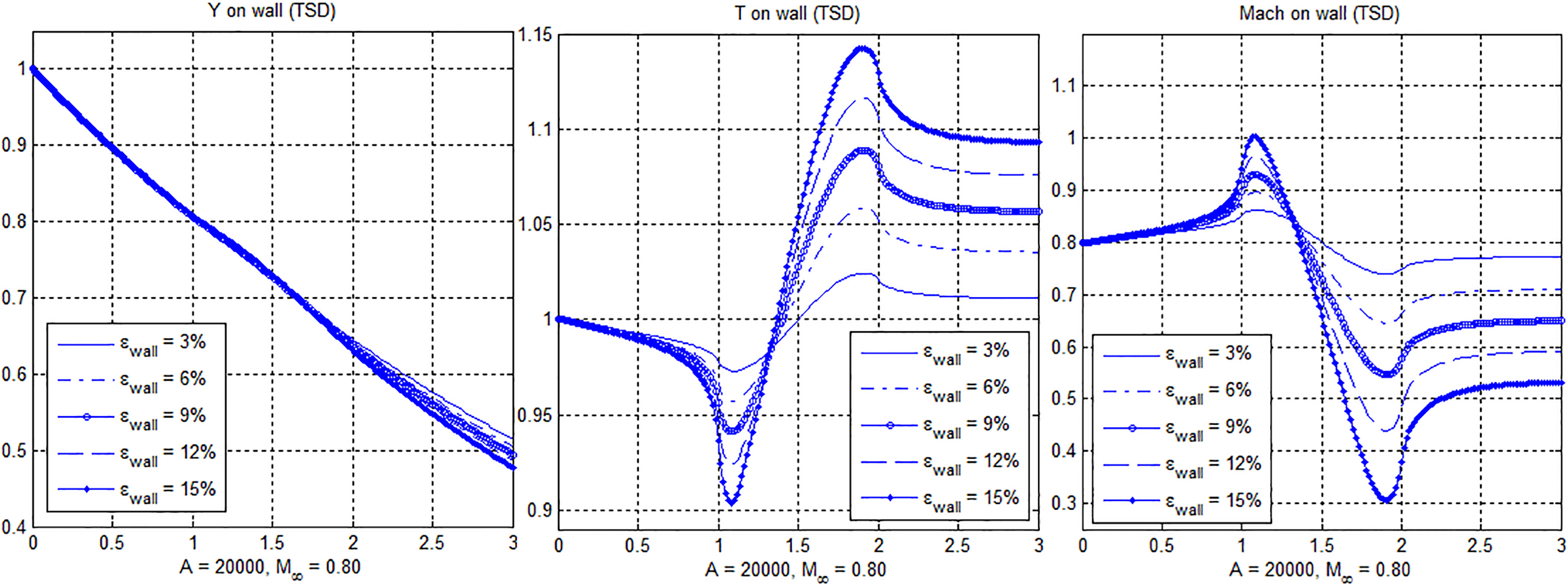
Small Disturbance Model (TSD) T and Y profiles for 0.80, 20000 for range of channel divergence parameters 3%, 6%, 9%, 12%, 15%. Higher channel divergence consumes more reactant (left) and results in a higher thermal energy (middle) and lower Mach number (right) at the outlet.
Along the channel walls:
As in [11] the nozzle geometry divergence is specified smoothly from a cosine continuation at :
Typically , unless otherwise specified, as in Fig. 3. We assume a symmetric flow, at the axis of symmetry, where :
In these calculations: , , . The mesh is 181 points in the -direction from to , and 101 points in the -direction from to . In this case, the 4-point operator of Murman-Cole is used to solve this mixed type elliptic hyperbolic equation with line successive under relaxation implicit in the -direction [9]. The reaction ODE is solved with Simpson’s integration method as in [11]. The Mach number is calculated by:
Non-reactive and reactive validation test cases are shown below and are in good agreement with [11]. Example results showing the transition from fully subsonic to shocked flow with a supersonic bubble for the non-reactive flow are given in Fig. 1.
As reported in [11], it is found that higher pre-exponential frequency factor consumes more reactant and results in a lower thermal energy and higher Mach number at the outlet, see Fig. 2. Higher peak Mach number as the duct is widening is also associated in this case with higher and higher reactant consumption.
Similarly, it is found that variation of the channel curvature through the factor consumes slightly more reactant and results in a higher thermal energy and lower Mach number at the outlet, see Fig. 3.
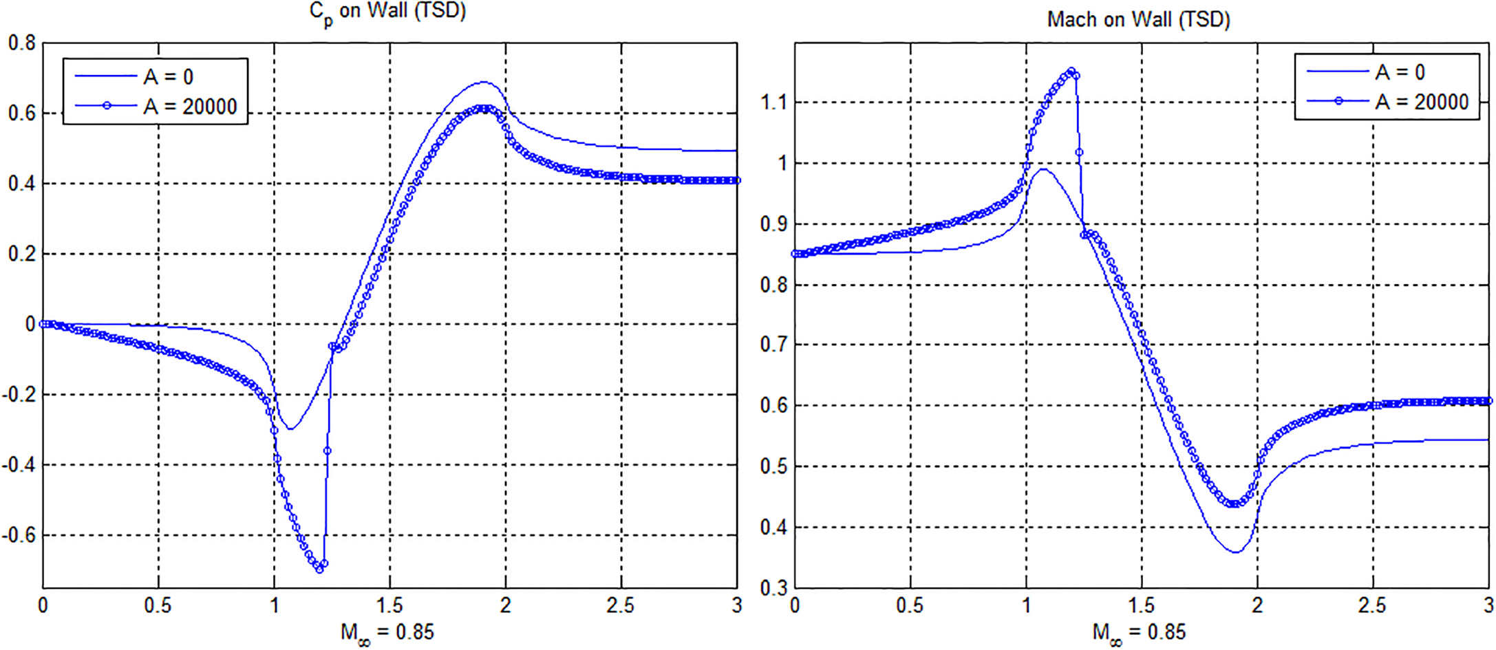
An important consequence of the heat release due to combustion is the capability to cause shocks as shown in Fig. 4. In this figure, for 0.85, without chemical reaction ( 0) the flow is completely subsonic and smooth, and with chemical reaction ( 20000) the flow contains a supersonic bubble which abruptly becomes subsonic through a normal shock. The outlet Mach number is higher and the outlet coefficient of pressure is lower for the reactive flow case where heat is released.
Small Disturbance Model (TSD), 0.85, 0 and 20000, shows supersonic bubble due to chemical reaction and small Zierup Singularity.
Numerical methods for the full potential model
To solve the full potential equation we use the artificial compressibility methods [4, 13]. We consider the density biasing and flux biasing formulations.
A modified artificial density method that is based on flux biasing is given by:
After calculating the local Mach number at the cell centers:
The flux is calculated at the cell-centers from:
Where the following definitions are used:
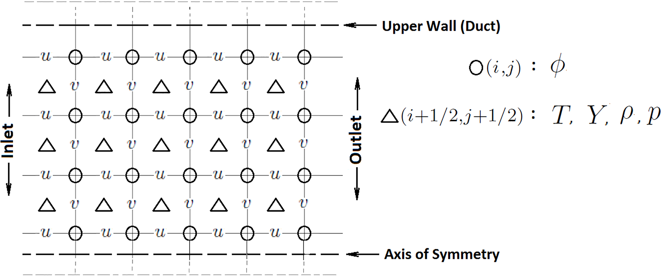
Staggered grid showing the location of the duct, centerline and model variables.
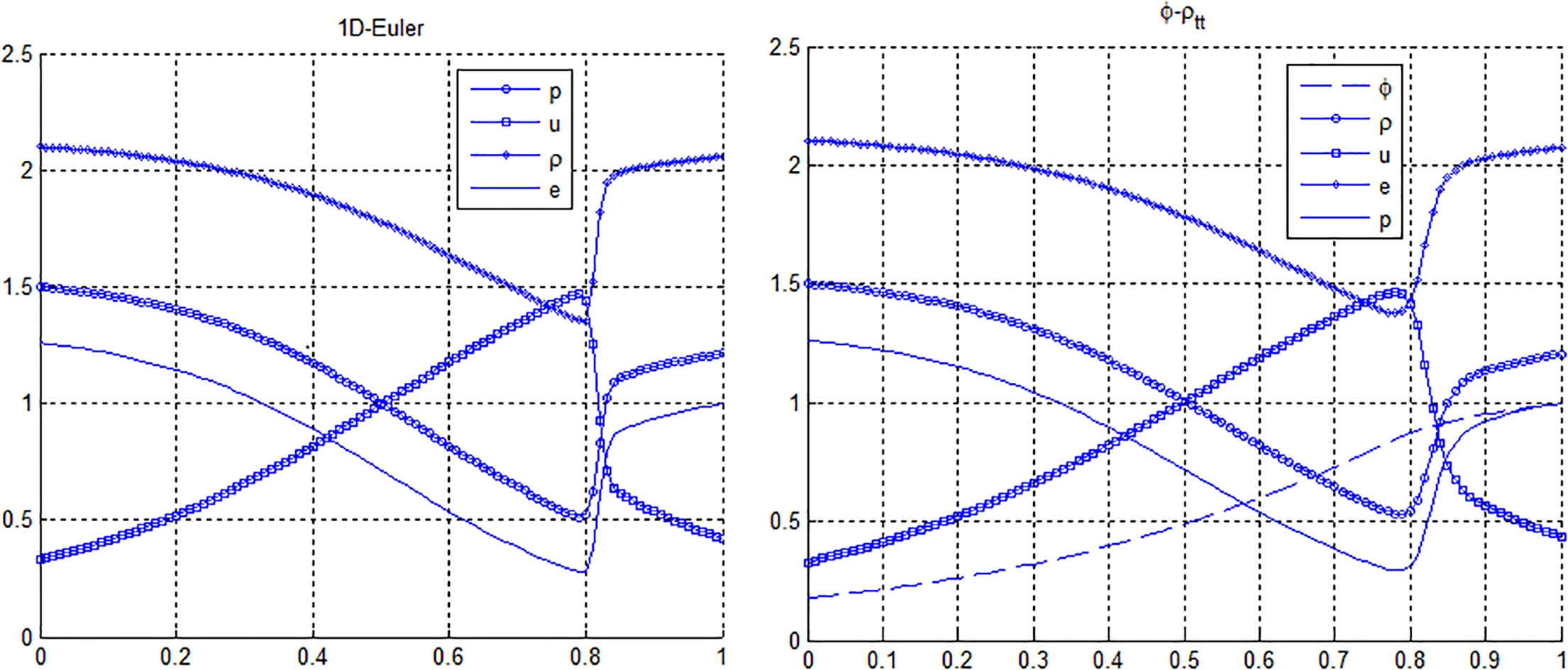
Compressible nozzle flow 1D validation test case. Quasi-1D Euler equations (left) and the quasi-1D full potential model (right).
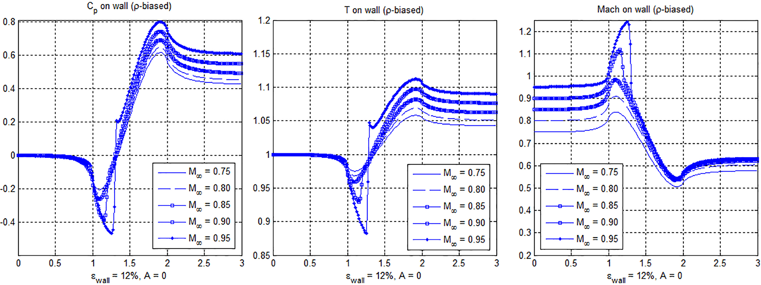
-biased full potential model for 0.75, 0.80, 0.85, 0.90, 0.95 for 0, showing transition to shocked flow at 12% nozzle area variation parameter.
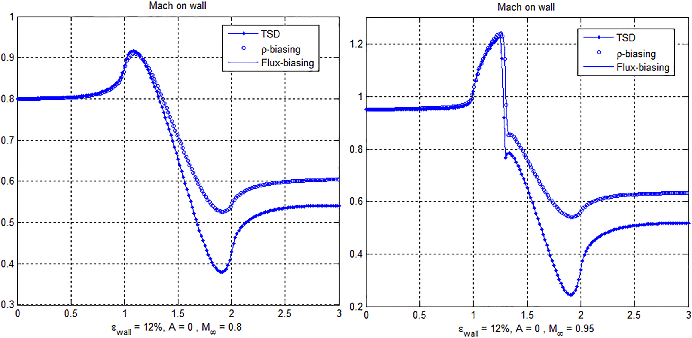
Flux Biasing and -Biasing vs. TSD with 0 for 0.8 (left) and for 0.95 (right).
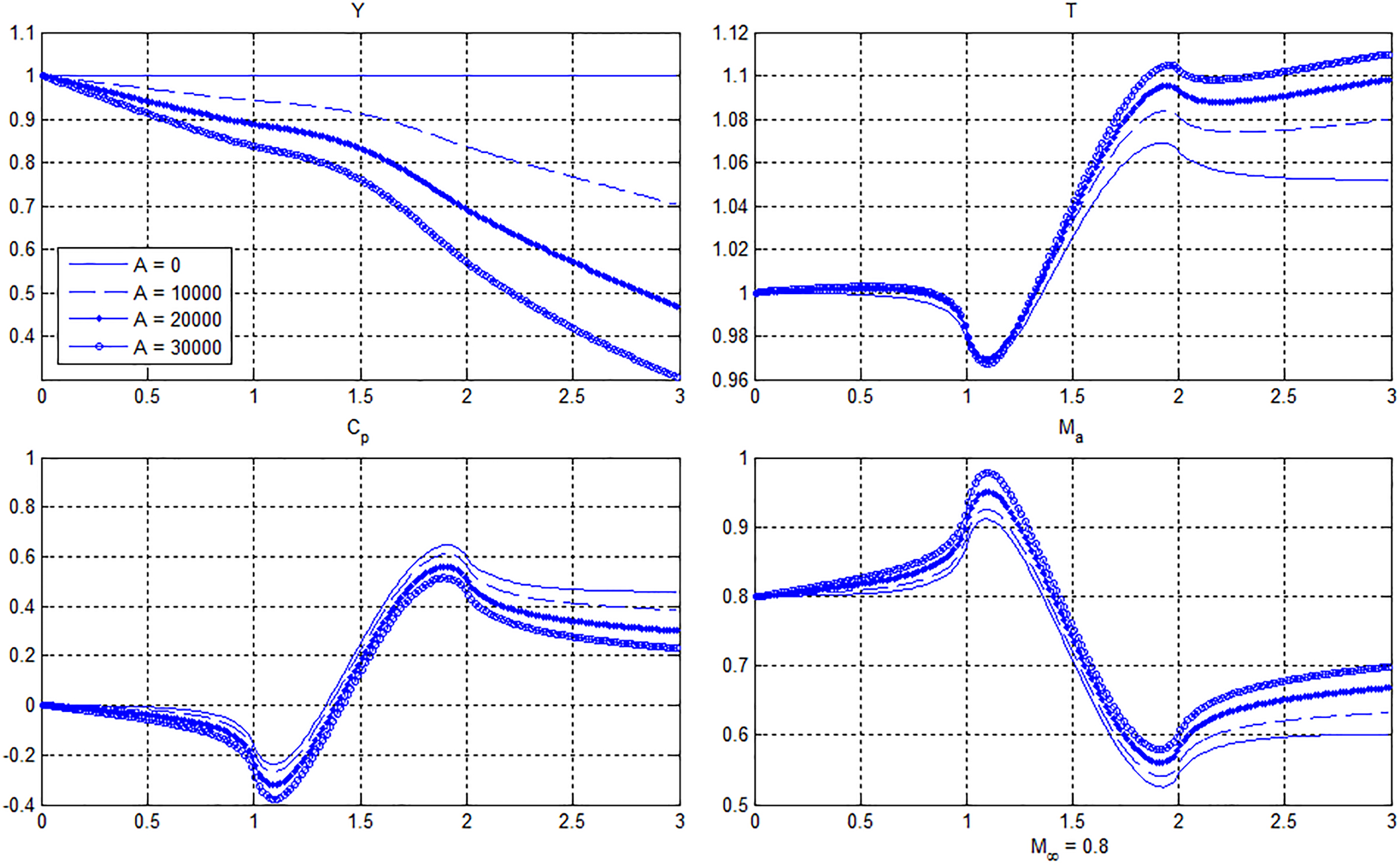
-biased full potential model with 0.8 for 0, 10000, 20000, 30000.
-biased full potential model with 0.85 for 0, 10000, 20000, 30000.
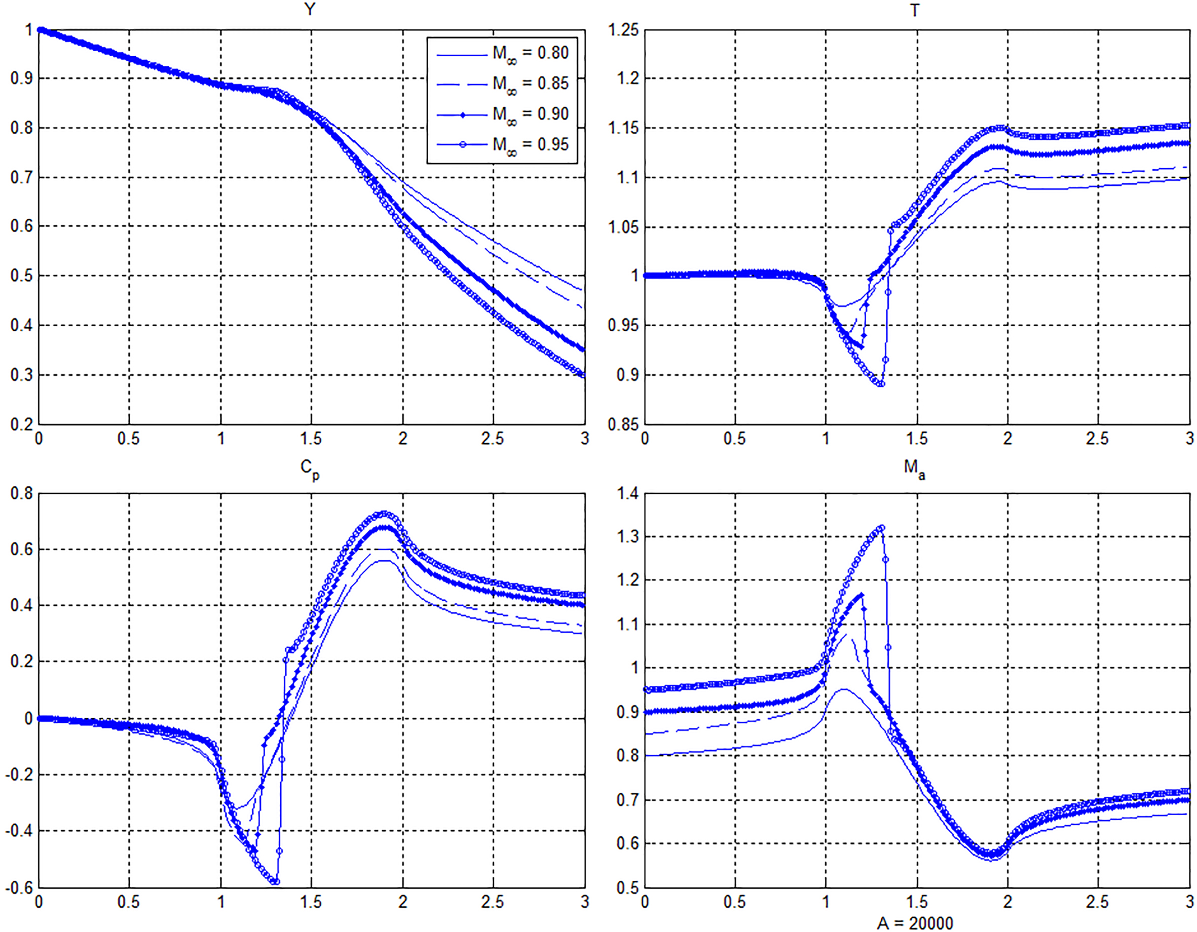
-biased full potential model for 0.80, 0.85, 0.90, 0.95 with 20000.
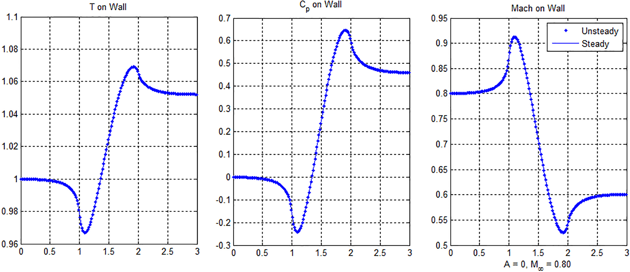
-biased unsteady full potential model for 0.80 with 0 validating the unsteady model converges to the same steady state solution.
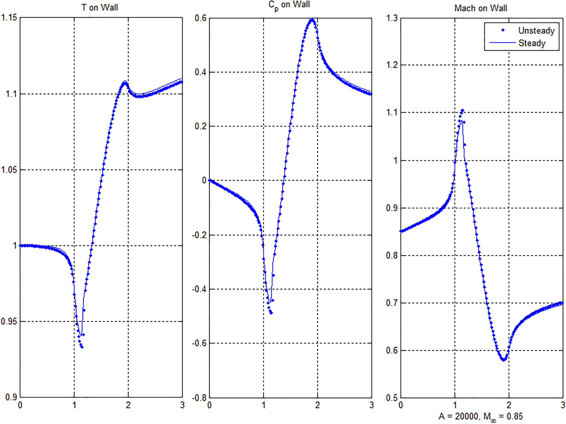
-biased unsteady full potential model for 0.85 with 20000 showing the steady state and unsteady solution overlayed.
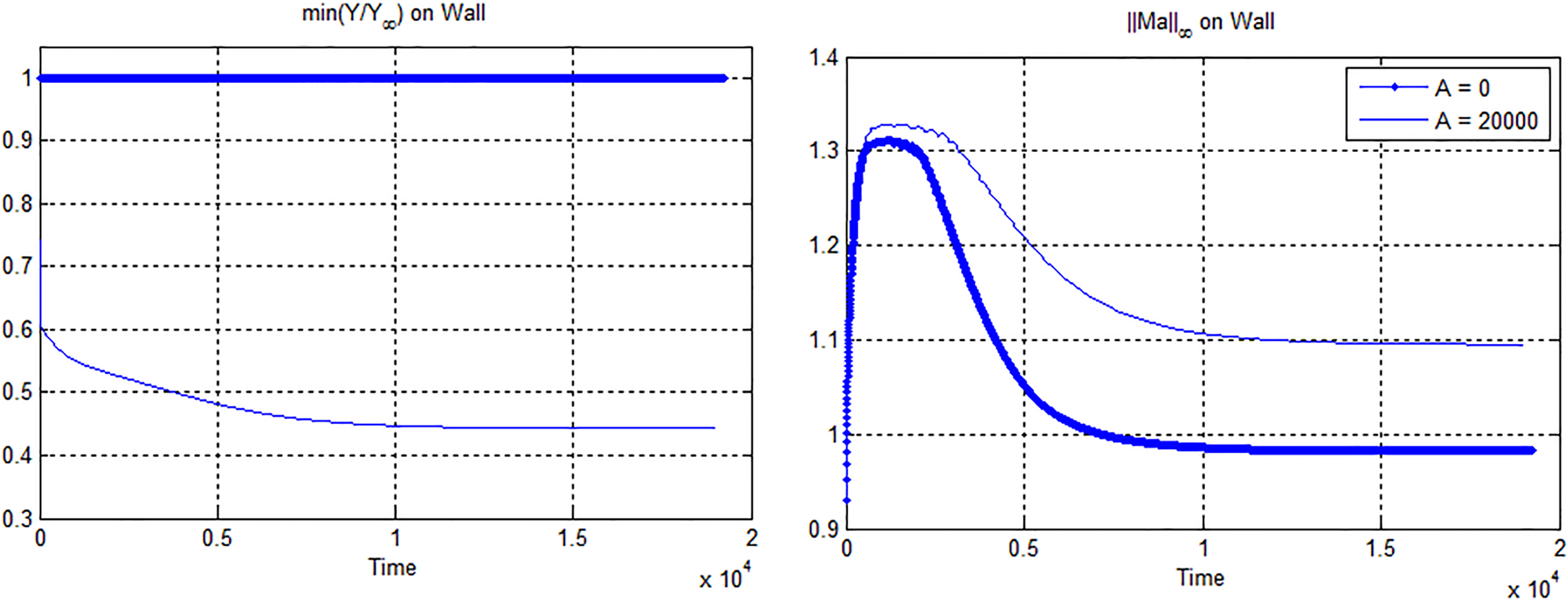
Unsteady peak Mach number (right) and minimum Y value (left) along the wall for 0.85 with 0, 20000. It is shown that the unsteady code converges from quiescent initial conditions to the same solution as the steady code.
In the density biasing scheme, instead of biasing the flux , now the density alone is biased:
Where the upwind shifting parameter is defined in terms of the local Mach number [5]:
Where , are user specified parameters. The energy and species equations are solved using a conservative mixed upwind/centered scheme with backward difference in the -direction. A staggered grid is used as show in Fig. 5.
For the case of steady state computations, all the time dependent terms are removed from the governing equations. The pressure Poisson equation is solved for :
and the density is updated via the perfect gas law by line successive under relaxation until convergence, where denotes the iteration count:
Since the the pressure, temperature and species equations are elliptic, they are iteratively solved until convergence before updating the potential function again, and then recalculating the velocity field.
For the case of unsteady computations a stability term of the form: , with , is added to the pressure equation to help with convergence:
This term is a natural choice because when small viscosity is present in the momentum equations:
Where . One way to proceed is that the pressure equation is solved for and the gas law is used to update . The other, which has the advantage of being able to treat operators implicitly, is to solve the pressure equation for and update the density from the gas law. In this case, one must first update the temperature to the current time step, , then, using the gas law, is solved according to the nonhomogeneous wave equation:
Boundary conditions, in terms of the standard momentum equations, must be used to eliminate spurious solutions.
1D Euler vs. 1D unsteady full potential
A validation test case is performed in 1D and compared against the quasi-1D Euler equations following the example given in [2]. We write the energy equation in terms of temperature using the relation:
Then the energy equation becomes:
Differentiation of conservation of mass with respect to and conservation of momentum with respect to , inclusive of artificial viscosity terms, gives:
Adding these equations together implies:
Therefore, the present pressure based model for the quasi-1D Euler Equations and small artificial viscosity (with strength ) is given by:
This system is hyperbolic and converges with . Alternatively, one can solve the continuity equation for a potential function , where , without loss of generality as is proposed earlier.
A comparison showing the quasi-1D Euler equations (left) and the quasi-1D full potential model (right) is shown in Fig. 6. The correct shock location ( 0.82) and flow through the sonic point is acheived in both models, see [2].
Results of the present two-dimensional full potential model
The small disturbance model is essentially mixed type in the -direction only. In contrast, the full potential can handle mixed type flows in multiple principal directions. As in the small disturbance model, a validation case showing the transition from fully subsonic to shocked flow with a supersonic bubble for a non-reactive flow case is shown first in Fig. 7.
When the full scheme is used, the results are slightly different from the small disturbance model, although the shock location prediction as well as peak Mach numbers are similar. The pre-shock solution and shock location are very similar, the post shock conditions are seen to vary between the TSD and full potential model, as shown in Fig. 8.
The profiles for and are markedly different from the TSD model. In particular, where the TSD model predicts that temperature trends like , in the full model, the temperature increases with heat release. The Y profiles are similar to that of the TSD model, but in our calculations there is a more noticeable effect of the geometry creating variation in reactant consumption rate.
In Fig. 9 the case of 0.8 for a range of pre-exponential frequency factors 0, 10000, 20000, 30000 is computed. This result is in good agreement with the small disturbance model.
In Fig. 10 the case of 0.85 for a range of pre-exponential frequency factors 0, 10000, 20000, 30000 is computed. In this case, the results show the combustion induces a supersonic flow bubble. The trend with respect to Mach number and pressure coefficient are in agreement with the small disturbance model. As in the case with the TSD model, without chemical reaction ( 0) the flow is completely subsonic and smooth, and with chemical reaction a supersonic bubble is shown to develop, the outlet Mach number is higher and the outlet coefficient of pressure is lower for the reactive flow cases where heat is released.
In Fig. 11 the case of incident -biased full potential model for 0.80, 0.85, 0.90, 0.95 with 20000 is computed.
An unsteady example has been computed as a validation test for 0.80 with 0. The results are in good agreement with the steady state model and are shown in Fig. 12.
Also the case where combustion causes a shock in the flow for 0.85 with 20000 has been computed. The results are shown in Fig. 13 and indicates the unsteady model produces a slightly sharper shock that is in nearly the same location as the steady model.
The time dependent transient history for 0.85 with 20000, starting from uniform quiescent initial data show the effect of combustion on the peak Mach number and fuel consumption in Fig. 14. This result shows that the steady state exists and that startup can cause shocked flow, but the long time behavior of the solution is not dependent on this transient behavior.
Conclusions
It is clear that the small disturbance approach is limited to small heat release and small area variation. Although the small disturbance model is limited in its range of applicability, within that range it is simpler to apply and can produce quite reasonable results, see [11]. The full potential model is more general and should be able to handle a larger heat release and area variation as indicated in the text. In addition, it should be straightforward to include a more detailed reaction mechanism without significant modifications to the model.
In the present work we have developed a full potential model with chemical reactions and numerical methods for its solution, including cases with strong sharp shocks. Moreoever, we introduced a new scheme based on pressure correction using a hyperbolic equation and the results have been verified for an unsteady one dimensional problem. The merits of the new formulation compared to the standard elliptic equation for the pressure are discussed.
References
1.
BuckmasterJ. and LudfordG., Theory of Laminar Flames, Cambridge University, 1982.
2.
ChattotJ.J., Computational Aerodynamics and Fluid Dynamics, Springer-Verlag Berlin Heidelberg New York, 2002.
3.
ColeJ.D. and CookL.P., Transonic Aerodynamics, Elsevier Science Publishers B.V., 1986.
4.
HafezM.M.SouthJ. and MurmanE.M., Artificial Compressibility Methods For Numerical Solution of Transonic Full Potential Equation, AIAA Journal17(8) (1979), 838–844.
5.
HafezM.M.HabashiW.G. and KotiugaP.L., Conservative calculations of non-isentropic transonic flows, International Journal for Numerical Methods in Fluids5 (1985), 1047–1057.
6.
HolstT.L., Numerical Computation of Transonic FLow Governed by the Full-Potential Equation, (N83-19708) NASA Technical Memorandum 84310, 1983.
7.
KuoK.K., Principles of Combustion, John Wiley & Sons, Inc, 2005.
8.
LiepmannH.W. and RoshkoA., Elements of Gasdynamics, Dover, 2012.
9.
MurmanE.M. and ColeJ.D., Calculation of Plane Steady Transonic flow, AIAA S.9(1) (1971), 114–121.
10.
OsherS.HafezM.M. and WhitlowW., Jr., Entropy Condition Satisfying Approximations for the Full Potential Equation of Transonic Flow, Mathematics of Computation44(169) (1985), 1–29.
11.
RusakZ.LeeJ.C. and ChoiJ.J., A small-disturbance model of transonic combustion, Combustion Theory and Modeling12(1) (2007), 93–113.
12.
RusakZ. and LeeJ.C., Parametric Investigation of Combustion in Compressible Flows, AIAA-2005-4805: 4th AIAA Theoretical Fluid Mechanics Meeting, 2005.
13.
VolpeG. and JamesonA., Transonic Potential Flow Calculations by Two Artificial Density Methods, AIAA Journal26(4) (1988).