Comparative investigations into dynamic rheological modeling of the water-based drilling fluid under HTHP conditions

Abstract

An accurate HTHP rheological model is essential for safe and economical deep drilling. In this work, the water-based fluid applied in Southwest China Gas Fields is selected as a typical example to systematically explore rheological modeling at elevated temperature(up to 180 ${}^{\circ}$ C) and pressure(up to 100 MPa). The HTHP rheological behavior of water-based drilling fluid was firstly investigated. Then general rheological modeling approaches and specific HTHP modeling process have been employed to establish an accurate HTHP rheological model. The results showed that for general rheological models, the Bingham model appears to be more suitable to predict the transient rheology at constant conditions; under HTHP conditions, a dynamic rheological model has been established using the relative dial reading method modified by the direct fitting, whose prediction deviation was in the range of $-$ 7.13% $\sim$ 10.63%, meeting in-field application requirements well. This research will be useful to direct a comprehensive rheological treatment, and will also enrich the modeling strategy of HTHP rheology for drilling fluids.

Keywords

HTHP dynamic rheological models water-based drilling fluid deviation

1. Introduction

The past few years have witnessed a rapid widespread for the deep drilling in China, especially in the southwest region, due to an increased demand for hydrocarbon energy. Generally, the deep gas drilling readily encounters harsh downhole environments, particularly the high temperature and high pressure (HTHP), which may severely affect properties of drilling fluids and the drilling progress. Hence, it is significant to maintain moderate properties of drilling fluids under the extreme conditions [1].

The rheology, as an important property of drilling fluids, appears to be critical for the successful drilling of deep, hot wells. Reasonable control of rheology is essential in most drilling operations, e.g., hydraulic calculation, pressure loss calculation, hole cleaning efficiency, and equivalent circulating density (ECD) determination, which enable high rate of penetration (ROP) and low drilling cost. The determination of rheologcal data relies, to a large extent, on a rheological mathematic representation, which allows an accurate theoretical prediction. Therefore, rheological modeling usually behaves as the first step in the HTHP drilling operation. However, it is well-known that in deep operations, rheology of drilling fluid is relatively complicated and often influenced by temperature, pressure, shear history, and composition of the drilling fluid [2, 3, 4]. Otherwise, temperature and pressure effects on rheology of drilling fluids are much different in downhole. As a result, HTHP rheological modeling can be restrained by complex fluid behaviors.

In the current work, rheological modeling has been examined based on the water-based drilling fluid applied in Southwest Gas Fields in China. A systematic investigation from rheological variation with temperature and pressure, selection of transient rheological models at constant temperatures and pressures, to a detailed comparison of dynamic rheological models, has been conducted, for the purpose of improving HTHP rheological modeling strategy. A newly modeling process has been developed, based on the modified HTHP rheological models. The literature linked with HTHP models has been firstly reviewed, which would be helpful to understand the profiles of HPHT rheological modeling.

1.1 HTHP rheological modeling progress

In view of the application mode, HTHP rheological models can be divided into two classes: the transient and dynamic models. The former is based on mathematical equations relating shear stress ( $\tau$ ) and shear rate ( $\gamma$ ) at the given condition, chiefly including two- and three-parameter traditional models such as Newtonian, Bingham Plastic, Power Law, Casson, and Herschel-Bulkley Models, etc. The transient models have been greatly improved by adding the more parameters (e.g., four parameter models) for better accuracy. Even so, it is relatively limited in practical prediction, due to a lack of T/P factors. Therefore, some effects have been made to enhance dynamic prediction of HTHP rheological models in downhole.

In general, introducing T/P correction into traditional models is the most direct way, which can modify rheological models by three variable equations. At present, the two HTHP rheological modeling, multiplicative factor (MF) and relative dial readings (RDR) methods, have been developed in terms of such modification strategy.

The common MF expression is given in,

$\displaystyle f(P,T)=\exp\left(\frac{A+(BT+C)P}{T}\right)$ (1)

where $A$ , $B$ , and $C$ are characteristic constants. Following Eq. (1), McMordie et al. [5] modified the power-law model as,

$\displaystyle\ln\tau=\ln K^{\prime}+n\ln\gamma+AP+B/T$ (2)

where $K^{\prime}$ and $n$ correspond to the consistency index and behavior index, respectively. This HTHP rheological model has been successfully used in the oil-based drilling fluid. Similarly, Houwen and Geehan [6], Hiller [7], and Alderman et al. [8] have applied the MF method to the two-parameter Casson and Bingham plastic models, as well as three-parameter Hurschel-Bulkley and Robertson-Stiff models. On the basis of modeling procedure and results, they concluded that the correlation of parameters in base equations can disturb the final precision of prediction.

To diminish the correlation of parameters, Rommetveit and Bjorkevoll [9]proposed another way to construct base equation, which is written as,

$\displaystyle f(P,T,\gamma)=e^{g_{1}(P,T)}\gamma+e^{g_{2}(P,T)}$ (3)

where $f(P,T,\gamma)$ is a factor that multiplies shear stress at standard conditions at the actual shear rate $\gamma$ . The constant functions $g_{1}(P,T)$ and $g_{2}(P,T)$ are determined by a best fit to measured data. In this case, the intrinsic defects of the selected base models can be avoided, which makes prediction more accurate.

Also, such modeling approach is recommended in the American Petroleum Institute (API) and the HTHP rheological model is,

$\displaystyle\tau(T,P,\gamma)=\tau_{o}(\gamma)e^{[\alpha(T-T_{o})+\beta(P-P_{o% })]}$ (4)

where $\tau_{o}$ denotes the shear stress at a given rotational speed. Further, Eq. (4) is extended to of viscosity expressions. For examples, on the basis of Stiff and Henry [10] and Johnston [11] assumptions, Minton and Bern [12] derived a corrected viscosity equation for the oil-based drilling fluid, which is presented as follows,

$\displaystyle\mu(T,P)=\mu_{o}e^{[\alpha(T-T_{o})+\beta(P-P_{o})]}$ (5)

where $\mu_{o}$ , $T_{o}$ , and $P_{o}$ separately correspond to viscosity, temperature, and pressure values under the reference conditions. Equation (5) has been widely used for viscosity prediction in downhole [13, 14].

Another HTHP modeling approach is the RDR method developed by Hemphill [15], which has been used to predict rheological behaviors of ester-based drilling fluids. The RDRs are defined as,

$\displaystyle\textit{RDR}=\frac{\theta_{T,P}}{\theta_{T_{o},P_{o}}}$ (6)

where $\theta$ is the dial reading and $T_{o}$ and $P_{o}$ are the reference temperature and pressure. In RDR modeling, it is not necessary to use a rheological model as the base equation, and thus, the assumption of base rheological model can be avoided. Combining with Arrhenius Relation, the RDR model is shown as follows,

$\displaystyle\textit{RDR}(T,P,\gamma)=C_{1}(P,\gamma)\exp[(C_{2}(P,\gamma))/T]$ (7)

where $C_{1}$ and $C_{2}$ are model coefficients that are dependent on the pressure and shear rate. The RDR model has been successfully utilized for defining rheological properties of synthetic-based drilling fluids under HTHP conditions by Barkim [16]. Also, Xu et al. [17] validated the RDR application in the sulphated water-based drilling fluids. A transfer of rheological modeling from physical models to mathematical calculation is the important trend. Using the mathematical method, Zhou et al. [18] established a comprehensive predictive model for the oil-based drilling fluid, which can be applicable for all common rheological model.

To sum up, all HTHP rheological models are closely contacted with physical and mathematic views in nature. It should be pointed out that previous studies on HTHP rheological modeling were chiefly concentrated on methodology, while systematic modeling application is rarely referenced. Meanwhile, HTHP rheological models are primarily performed on the oil-, synthetic-, and invert emulsion-based drilling fluids rather than the water-based drilling fluids. Therefore, a systematic investigation into HTHP rheological modeling for the water-based drilling fluids can not only enrich rheological knowledge, but also provide a modeling strategy for establishing accurate HTHP rheological models for water-based drilling fluids.

2. Materials and methodology

2.1 Water-based drilling fluid

The field water-based drilling fluid has a density of 1.5 g/ml, and it consists of at least 7 functional additives, such as hydrophilic solid phase, pH control agent, loss control agent, viscosifier, inhibitor, antioxidant, and weighting material (see Table 1). To enhance the temperature resistance, most polymeric additives underwent the sulphonated treatment. The prepared sample was heat-aged at 180 ${}^{\circ}$ C for 16 hours before testing.

2.2 Design of experiments

In the target reservoir, the geothermal gradient ranges between 2.3 $\sim$ 2.5 ${}^{\circ}$ C per 100 m, and numerous well depths are as high as 6,000 m. Considering extreme downhole environments, herein, testing temperature up to 180 ${}^{\circ}$ C and pressure up to 100 MPa have been designed. Pressures applied during the tests were 15 MPa, 25 MPa, 55 MPa, 85 MPa, and 100 MPa, and temperatures applied during tests range between 60 $\sim$ 180 ${}^{\circ}$ C. Using a Fann IX77 HTHP Rheometer, rheology of the drilling fluid was measured at six specific shear rates (600 rpm, 300 rpm, 200 rpm, 100 rpm, 6 rpm, and 3 rpm) under each T/P condition.

2.3 Modeling methods

The MF and RDR approaches mentioned above have been employed to build dynamic rheological models, wherein the $T/P$ correction is added. The model should mathematically describe the relationship between a dependent variable ( $\tau$ ) and its regressor variables ( $T$ , $P$ , and $\gamma$ ). The standard procedure for rheology modeling is usually through nonlinear regression of rheological data. This is generally done using a numerical package such as Spss, Matlab, or Statistic software, by minimizing the sum of square errors and judging the goodness of the fit through the evaluation of the correlation coefficient ( $R^{2}$ ), residual values, and error percentages. Note that, multiple linear or nonlinear regression technique can be adopted based on the intrinsic relation between rheological properties and $T/P$ effects. On account of requirements of accuracy, different expressions like logarithmic, exponential, and polynomial model can be obtained upon fitting (vide infra).

Table 1
Main components for the water-based fluid

Additives	Ingredients	Content (wt.%)
–	Water	–
–	Clay	4 $\sim$ 5
pH-adjusting agent	Sodium hydroxide	0.5
Main viscosifier	PAMS copolymer	1.0
Viscosifier	Amphoteric sulfonated polymer	0.5
Filtrate loss reducer	Sulfonated phenolic resin	4
–	Lignosulfonate	4
Weighting material	Barite	–

Table 2

Fann viscometer: dial readings measured under different HPHT conditions ${}^{\text{a}}$

P (MPa)	T ( ${}^{\circ}$ C)	Shear rates ${}^{\text{b}}$ (rpm)
		600	300	200	100	6	3
100	60	116(0.5577)	87(0.5241)	77(0.5238)	66(0.5410)	53(0.5761)	53(0.6023)
100	90	68(0.3269)	47(0.2831)	39(0.2653)	32(0.2623)	25(0.2717)	24(0.2727)
100	120	49(0.2356)	31(0.1867)	25(0.1701)	18(0.1475)	13(0.1413)	13(0.1477)
100	150	38(0.1827)	21(0.1265)	16(0.1088)	11(0.0902)	7(0.0761)	7(0.0795)
100	180	32(0.1538)	16(0.0964)	11(0.0748)	7(0.0574)	4(0.0435)	4(0.0455)
85	60	117(0.5625)	88(0.5301)	78(0.5306)	67(0.5492)	54(0.5870)	53(0.6023)
85	90	68(0.3269)	47(0.2831)	39(0.2653)	32(0.2623)	25(0.2717)	24(0.2727)
85	120	49(0.2356)	31(0.1867)	25(0.1701)	18(0.1475)	13(0.1413)	13(0.1477)
85	150	38(0.1827)	21(0.1265)	16(0.1088)	11(0.0902)	8(0.0870)	7(0.0795)
85	180	32(0.1538)	16(0.0964)	11(0.0748)	7(0.0574)	4(0.0435)	4(0.0455)
55	60	117(0.5625)	87(0.5241)	77(0.5238)	66(0.5410)	53(0.5761)	52(0.5909)
55	90	68(0.3269)	47(0.2831)	40(0.2721)	33(0.2705)	25(0.2717)	24(0.2727)
55	120	49(0.2356)	31(0.1867)	26(0.1769)	19(0.1557)	14(0.1522)	13(0.1477)
55	150	38(0.1827)	22(0.1325)	17(0.1156)	12(0.0984)	8(0.0870)	7(0.0795)
55	180	32(0.1538)	17(0.1024)	12(0.0816)	7(0.0574)	4(0.0435)	4(0.0455)
25	60	117(0.5625)	87(0.5241)	77(0.5238)	66(0.5410)	53(0.5761)	52(0.5909)
25	90	68(0.3269)	47(0.2831)	40(0.2721)	33(0.2705)	25(0.2717)	24(0.2727)
25	120	49(0.2356)	31(0.1867)	26(0.1769)	19(0.1557)	14(0.1522)	13(0.1477)
25	150	38(0.1827)	22(0.1325)	17(0.1156)	12(0.0984)	7(0.0761)	7(0.0795)
25	180	32(0.1538)	17(0.1024)	12(0.0816)	8(0.0656)	4(0.0435)	4(0.0455)
15	60	115(0.5529)	86(0.5181)	76(0.5170)	65(0.5328)	53(0.5761)	52(0.5909)
15	90	68(0.3269)	47(0.2831)	40(0.2721)	33(0.2705)	25(0.2717)	24(0.2727)
15	120	49(0.2356)	31(0.1867)	25(0.1701)	18(0.1475)	14(0.1522)	13(0.1477)
15	150	38(0.1827)	22(0.1325)	17(0.1156)	12(0.0984)	8(0.0870)	8(0.0909)
15	180	32(0.1538)	17(0.1024)	12(0.0816)	8(0.0656)	4(0.0435)	4(0.0455)
0.1	30	208(1)	166(1)	147(1)	122(1)	92(1)	88(1)

${}^{\text{a}}$ Values in brackets denote RDRs. ${}^{\text{b}}$ Shear stress is given in Pa.

3. Discussion and results

3.1 HTHP Rheological characterization

Table 2 collects the dial reading and RDR values under the considered conditions. As might be anticipated, the water-based fluid is rarely pressure-dependent and highly temperature-dependent. For example, in the pressure range of 15 $\sim$ 100 MPa, the average changes of dial readings from 600 rpm to 3 rpm are, respectively, 0.83 Pa, 0.33 Pa, 0.17 Pa, 0.83 Pa, and 0.50 Pa at 60 ${}^{\circ}$ C, 90 ${}^{\circ}$ C, 120 ${}^{\circ}$ C, 150 ${}^{\circ}$ C, and 180 ${}^{\circ}$ C, the magnitude of which is less than 1. Apparently, the impact of pressure on rheology is relatively little. Interestingly, pressure effects on rheology can slightly rise at high temperature and low shear rates. At 150 ${}^{\circ}$ C, for example, changes of dial readings from 600 rpm to 3 rpm are, in turn, equal to 0%, 4.54%, 5.88%, 8.33%, 12.5%, and 12.5%, as in creasing pressures. While at 60 ${}^{\circ}$ C, the dial reading variations are 0.9%, 1.1%, 1.3%, 1.5%, 1.9%, and 1.9%, respectively, on going from 15 MPa to 100 MPa. It is clear in the water-based drilling fluid that, the rheological parameters appear to be low pressure-sensitive. Note that, this trend is very contrary to what happen in oil-based drilling fluid. Ibeh et al. [19] pointed out that in the oil-based drilling fluid, while varying the pressure from 35 MPa to 105 MPa, the variations of typical rheological parameters YP and PV tested at 75 ${}^{\circ}$ C were 100% and 89%, respectively. In the water-based drilling fluid, however, variations of YP and PV at 60 ${}^{\circ}$ C are only 3% and 1.7%, respectively, far less than variation of oil-based drilling fluid. The rheological property of water- and oil-based drilling fluids is closely related with the solution compression.

Despite a slight rise, effects of pressure on rheology can be ignored as compared with that of temperature. For instance, at each pressure, variations of dial readings at six shear rates rpm exceed 70%, when increasing temperature from 60 ${}^{\circ}$ C to 180 ${}^{\circ}$ C. Noticeably, the magnitude of variation is dramatically larger than that derived from pressure. This validates the fact that the effect of temperature on rheology is more dominant than that of pressure, in accordance with previous studies [8].

Figure 1 further visually compares the temperature and pressure effects on rheology. It is apparent that in Fig. 1, several regular color belts parallel to $P$ -axis may be observed at a constant temperature and, in this regard, each belt is filled with single color, indicative of less variation of dial readings with pressure. In addition, one easily observes that the three-dimensional surface exhibits different color sheets along $T$ -axis, which reflects a large change of dial readings as increasing temperature. Such unique color distribution can be viewed as an indicator of strong temperature dependence for rheology, which is well consistent with results described above.

Figure 1.

Effect of temperature and pressure on shear stress at different shear rates, the surfaces are colored on a blue-green-red (BGR) scale with respect to the magnitude of dial reading.

Inspection of Table 2 and Fig. 1 indicates that in the water-based systems, the pressure effect on rheology can be ignored in principle. However, the pressure variable ( $P$ ) is still kept in subsequent modeling, taking account of integrity of HTHP rheological models.

3.2 Transient HTHP rheological modeling analyses

Transient HTHP modeling generally denotes selection of the mathematic expression from the traditional models. It would be available in the targeted section because of the known downhole environment. Otherwise, understanding HPHT transient rheological model would be helpful to further construct the dynamic HPHT rheological model with T/P factors.

Herein, the 25 sets of dial readings listed in Table 2 were fitted to five typical rheological models, including the Bingham Plastic, Power Law, Casson, Herschel-Bulkley, and Robertson-Stiff models. Characteristic constants and correlation coefficients for various models are given in Table S1 (See supplementary material). As expected, the three-parameter models, Herschel-Bulkley and Robertson-Stiff models, are more reliable than the two-parameter models in extrapolation calculations. Their average correlation coefficients arrive at 0.9996 $\pm$ 0.0003 and 0.9995 $\pm$ 0.0003, respectively, suggesting excellent relationship between predicted and actual values. These results clearly demonstrate that the Herschel-Bulkley and Robertson-Stiff models are adequate for predicting the rheological parameters of water-based drilling fluids at constant temperatures and pressures.

Meanwhile, the two-parameter Bingham model also gives good fits to the experimental data and its correlation coefficients are all more than 0.99, which are compatible to the three-parameter models. That is to say, the Bingham model can be used to characterize the rheology at constant conditions. This finding is relatively different from the results attained in non-aqueous drilling fluids, wherein the Power Law model would perform well in predicating flow behaviors [20, 21].

3.3 Dynamic HTHP rheological modeling analyses

Dynamic HTHP rheological modeling means an incursion of T/P factors to the initial mathematic expression. As described above, two strategies, i.e., MF and RDR approaches, are usually used for establishing dynamic HTHP rheological models. In the oil industry, HTHP dynamic rheological models should be more popular and practical than the transient HTHP models.

3.3.1 MF approach

Establishment of general MF-corrected models is usually based on a transient base model. With the Arrhenius empirical relation, subsequently, the T/P correction factors are introduced to construct three-variable equation. This strategy has been used in the oil-based drilling fluid and, as a result, a MF-corrected Power Law model has been successfully established (see Eq. (2)). Here, the two-parameter Bingham and three-parameter Herschel-Bulkley models that are validated accuracy in the transient prediction, have been utilized to examine the general MF approach.

Table 3
Characterized constants of MF-corrected models

Based equations	Characterized constants
	$\tau_{y}$	$\mu_{p}$	$k$	$n$	$A$	$B$
Bingham	5.5408	1.4245 $\times$ 10 ${}^{-2}$	–	–	3.0089 $\times$ 10 ${}^{-5}$	131.0951
Herschel-Bulkley	5.3142	–	2.4175 $\times$ 10 ${}^{-2}$	0.9152	2.1256 $\times$ 10 ${}^{-5}$	132.0979

In view of the MF-corrected modeling, the dynamic HTHP rheological equations of Bingham and Herschel-Bulkley models can be determined as follows:

$\displaystyle\tau_{B}(P,T,\gamma)=(\tau_{y}+\mu_{p}\gamma)\exp(AP+B/T)$ (8) $\displaystyle\tau_{HB}(P,T,\gamma)=(\tau_{y}+k\gamma^{n})\exp(AP+B/T)$ (9)

where $\tau_{y}$ , $\mu_{p}$ , $n$ , and $k$ are characteristic parameters, and $A$ and $B$ are constants. These values may be determined by the least-squares approach.

Figure 2.

Statistic comparisons of error percentage for MF-corrected Bingham (top) and Herschel-Bulkley (bottom) models; the rhombus denotes the box (the inter-quartile region), the middle line denotes the median line, and the vertical lines denote the whisker.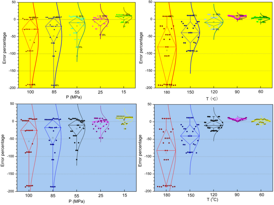

Table 3 presents all parameter and constant values in Eqs (8) and (9). As might be anticipated, the temperature constant B is the largest, which is about seven orders of magnitude larger than pressure constant A. This finding discloses the strongest correlation of temperature in the MF-corrected models, which is well consistent with results in Fig. 1. However, these two MF-corrected models yield poor agreement between measured and predicted values, as depicted in Fig. 2.

The established models have a low precision of prediction, especially at HTHP. For instance, the distribution of error percentage vs. $P$ shows that the location of the box is much closer to the upper whisker, reflecting the error percentage is mainly in the range of $-$ 50% $\sim$ 10%. Meanwhile, the median line is gradually far away from 0 as increasing pressure, suggesting that the precision of prediction reduce with pressure. In addition, there are at least 50% of error percentages between the media line and the lower whisker, which reveal that more than half of error percentages are lower than $-$ 20%. Further, the long lower whisker means a large error percentages (up to $-$ 190%). In the plot of error percentage vs. $T$ , two distribution properties of error percentages can be observed: 1) the majority of deviation is within the range of $-$ 80 $\sim$ $-$ 200%, 2) and the higher the temperature, the larger the error percentages are.

Similar to distribution of error percentages in the MF-corrected Bingham model, the MF-corrected Herschel-Bulkley model presents the large prediction deviation under the considered conditions, as shown in Fig. 2.

In terms of statistic population of error percentage, undoubtedly, the general MF approach fails to construct T/P-corrected rheological models. It should be ascribed to an unreasonable usage of Arrhenius empirical relation, which can impose the intrinsic restriction to the resulting models. Therefore, the MF modeling strategy would be modified by a direct approach of fitting variables to avoid uncertainty of assumed empirical relation.

On account of restriction of general MF approach, a direct fitting approach is used to establish the more accurate T/P dependence for each characterized constant, instead of the Arrhenius relation. Note that, this treatment involves nonlinear regression that demands a complex screening from logarithmic, exponential, and polynomial functions, which will minimize restriction of assumed equations. The modified rheolgical model expressions are given by

$\displaystyle\tau_{B}(P,T,\gamma)=\tau_{y}(P,T)+\mu_{P}(P,T)\gamma$ (10) $\displaystyle\tau_{HB}(T,P,\gamma)=\tau_{y}(P,T)+k(T,P)\gamma^{n(T,P)}$ (11)

where $\tau_{y}(P,T)$ , $\mu_{p}(P,T)$ , $k(P,T)$ , and $n(P,T)$ are characterized constant functions.

With characterized data listed in Table S3 characterized constants $\tau_{y}$ and $\mu_{p}$ in the Bingham model can be written as functions of T/P,

$\displaystyle\tau_{y}(P,T)=-10.8699-2.6987\times 10^{-3}P+1853.7649/T+122308.8% 459/T^{2}$ (12) $\displaystyle\mu_{P}(P,T)=-0.0151-0.013/P+15.6903/T-1083.402/T^{2}+34894.8/T^{3}$ (13)

Obviously, Eqs (12) and (13) are nonlinear polynomial functions, and both exhibit high correlation between actual and predicted values (0.9996 and 0.9990).

The error analyses of constant functions for the Bingham plastic model are presented in Table S3. Equations (12) and (13) predict the characterized constants with high accuracies under the investigated conditions. Notably, at 180 ${}^{\circ}$ C, Eqs (12) and (13) predict $\tau_{y}$ and $\mu_{p}$ with errors more than 7.42% and 6.82%, respectively, which can, to a large extent, affect the precision of prediction.

Similarly, characterized constant functions, $\tau_{y}(T,P)$ , $k(T,P)$ , and $n(T,P)$ , associated with the modified Herschel-Bulkley equation, are presented as follows,

$\displaystyle\tau_{y}(T,P)=-8.9671+1.6167/P+1.604\times 10^{3}/T+1.2274\times 1% 0^{5}/T^{2}$ (14) $\displaystyle k(T,P)=-0.9334+0.4348\ln P+99.3401/T-7.7\times 10^{-2}\ln^{2}P-4% .9858\times 10^{3}/T^{2}-18.0329\ln P/T+4.7\times 10^{-3}\ln^{3}P+9.4133\times 1% 0^{4}/T^{3}+6.7951\times 10^{2}\ln P/T^{2}+0.52\ln^{2}P/T$ (15) $\displaystyle n(T,P)=0.5423-0.7/P+8.8\times 10^{-3}T+1.3307\times 10^{2}/P^{2}% -5.7526\times 10^{-5}T^{2}-9.12\times 10^{-2}T/P-1.9361\times 10^{3}/P^{3}+2.0% 988\times 10^{-7}T-1.1204\times 10^{-4}T^{2}/P+1.3932T/P^{2}$ (16)

The coefficients of multiple determination for Eqs (14)–(16) are 0.9997, 0.9626, and 0.9654, respectively. Likewise, error analyses of constant functions for the modified Herschel-Bulkley model are given in supplement material(see Table S3). Obviously, $\tau_{y}(T,P)$ exhibits better prediction than $k(T,P)$ and $n(T,P)$ . In particular, $k(T,P)$ is the worse in prediction, and its error percentages range between $-$ 54.24% and 127.66%. It is worth noticing that the three constant functions generate severe deviation at 15 MPa. Substituting constant functions with Eqs (12)–(16), the HTHP rheological equation relating modified MF to downhole conditions ( $T/P$ ) and shear rate ( $\gamma$ ) can be determined.

Figure 3.

Box plots of error percentage vs. variable for the modified models attained by the defined MF approach; left: Bingham plastic model, right: Herschel-Bulkley model; In box plots of the modified Bingham plastic model, the 10th, 25th, 50th, 75th, and 90th percentile of deviation dataset are marked.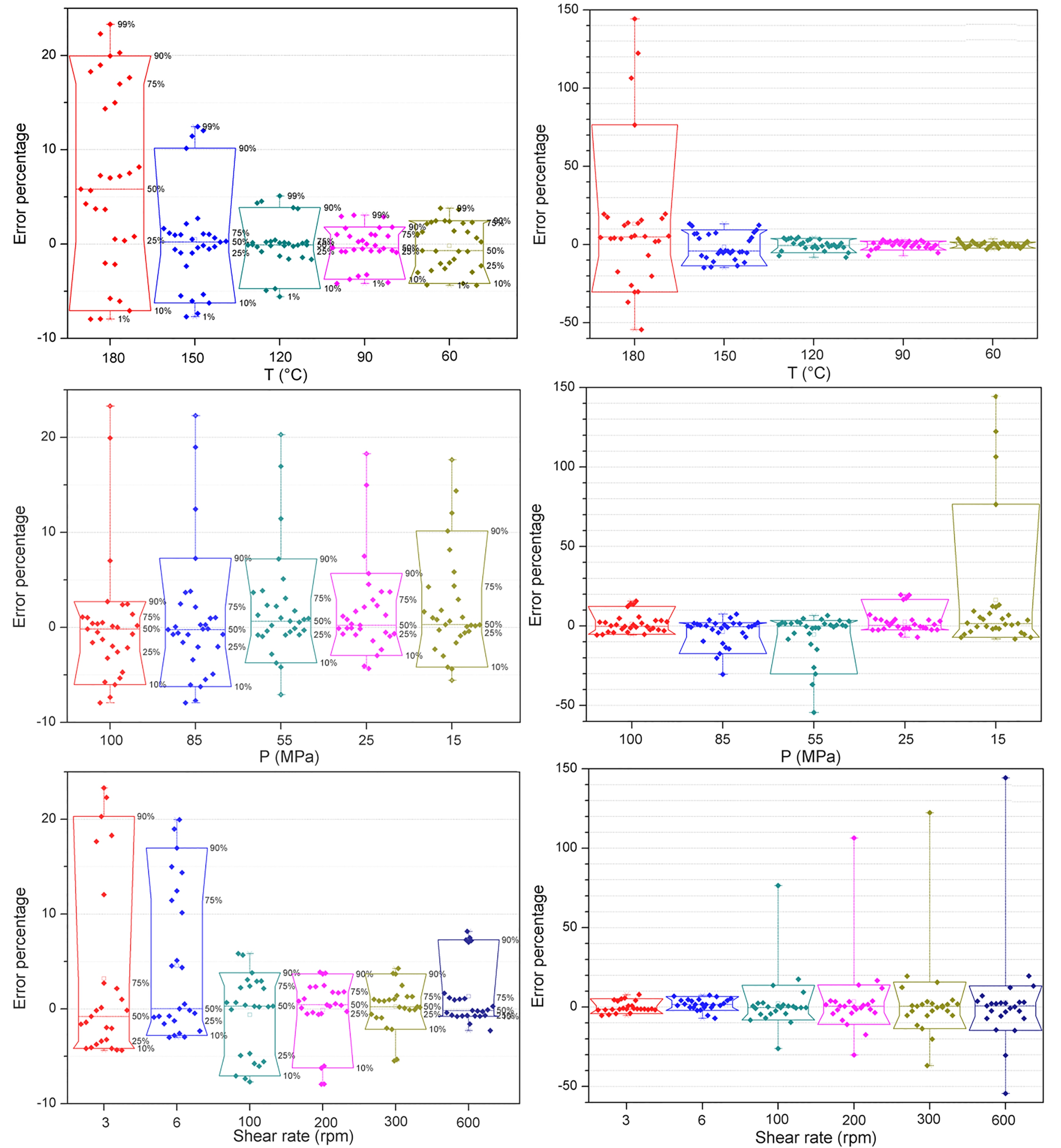

Figure 3 compares distribution of error percentages with respect to $T$ , $P$ , and $\gamma$ for the two modified models. It can be readily appreciated that the dynamic HTHP rheological models derived from modified-MF approach are more accuracy than from general MF approach. There is a considerable decrease in the range of error percentages and number of extreme values. On the basis of location of the median line, one can determine that the majority of prediction deviations are near to 0. These observations indicate that the direct approach of fitting can better improve accuracy of rheological models than empirical relations.

Furthermore, the modified Bingham model exhibits higher accuracy relative to the modified Herschel-Bulkley model. In the modified Bingham model, exceeding 90% of error percentages are in the range of $-$ 10% $\sim$ 10% and, synchronously, its extreme value is less than 25%; while in the modified Herschel-Bulkley model, the larger distribution of error percentages ( $-$ 30% $\sim$ 80%) may be observed, and its extreme value exceeds 150%. Additionally, comparing sizes of boxes in the modified Bingham model, one can observed that the model is temperature-, pressure-, and shear rate-dependent; as for the modified Herschel-Bulkley model, it appears to be more temperature- and pressure-dependent. As anticipated, the higher the temperature, the worse the prediction accuracy is, which agrees well with deviation of the characterized constants. In spite of large improvement, the modified MF modeling is still limited for establishment of accurate dynamic rheological models in the investigated conditions, due to presence of large extreme value.

The direct approach of fitting appears to be an effective strategy to improve HTHP rheological modeling by establishing accurate constant functions. Despite a large improvement, the dynamic HTHP rheological equations obtained by the modified-MF approach are limited due to their extreme values, which affect the prediction accuracy. To develop more reliable dynamic rheological models, we further carry out modeling on the basis of RDR approach.

3.3.2 RDR approach

The general RDR approach contains various fitting steps, especially the Arrhenius relation, which is previously verified to possibly damage accuracy of HTHP rheological model. Even so, we still established the dynamic HTHP models with the general RDR approach for modeling integrity. Herein, the ambient condition, i.e., 0.1 MPa and 30 ${}^{\circ}$ C, are viewed as the standard condition of RDR modeling.

Following the standard steps of RDR approach, the dynamic equation was built based on data listed in Table 2. As expected, a large deviation range of $-$ 104% $\sim$ 16% was obtained, which is, undoubtedly, ascribed to application of Arrhenius empirical relation. Its inaccuracy has been confirmed in modeling with the MF approach. The key to this problem is to establish a more accurate relation between RDR and $T$ . Nevertheless, multiple fitting steps can introduce more uncertainty in modeling.

Accordingly, we resort to another RDR approach proposed by Rommetveit and Bjorkevoll [9], through which fitting steps can be reduced. However, it also involves Arrhenius empirical relation in the constant functions. Hence, such RDR approach is modified by substituting exponential functions with a direct fitting function to T/P.

3.3.3 Modified RDR approach

The dynamic HTHP rheological expression based on the modified RDR approach is given by,

$\displaystyle\tau=[a(T,P)\gamma+b(T,P)]\times\tau_{s}$ (17)

where $\tau_{s}$ denotes dial readings at standard conditions, and $a(T,P)$ and $b(T,P)$ are coefficient functions.

Once the linear relation between $\tau/\tau_{s}$ and $\gamma$ under given conditions is determined, the coefficients $a$ and $b$ may be determined. All coefficients of correlation exceed 98.5%, suggesting a good linear relation between $\tau/\tau_{s}$ and $\gamma$ . The coefficient values are summarized in supplementary material (See Table S4), and a further direct fitting of $a$ , $b$ to variables $T$ and $P$ may determine coefficient functions.

$\displaystyle a(T,P)=2.0641\times 10^{-4}-2.6822\times 10^{-3}/T+2.8329\times 1% 0^{-7}P-0.5289/T^{2}+7.5108\times 10^{-10}P^{2}-2.881\times 10^{-5}P/T$ (18) $\displaystyle b(T,P)=-9.8321\times 10^{-2}+19.1033/T+1.173\times 10^{3}/T^{2}-% 2.8477\times 10^{-5}P$ (19)

Substituting Eqs (18) and (10) into Eq. (17), the final expression relating RDR to T/P and $\gamma$ can be determined,

$\displaystyle\tau=[(2.0641\times 10^{-4}-2.6822\times 10^{-3}/T+2.8329\times 1% 0^{-7}P-0.5298/T^{2}+7.5108\times 10^{-10}P^{2}-2.881\times 10^{-5}P/T)\times% \gamma+(-9.8321\times 10^{-2}+19.1033/T+1.173\times 10^{3}/T^{2}-2.8477\times 1% 0^{-5}P)]\times\tau_{s}$ (20)

As a next step, the accuracy of the developed model is investigated. Figure 4 compares error percentages versus temperature and pressure.

The error percentages vary ranging from $-$ 7.13% to 10.63%, and the average of absolute error percentages is 3.5304% $\pm$ 2.1767%. All deviation data evenly distribute along 0 at the given condition, and the only value tested at 15 MPa, 150 ${}^{\circ}$ C exceeds 10%. These results disclose that such model makes good prediction and can meet the field application well. Furthermore, this extreme point can be rarely encountered, taking into account the geothermal gradient and formation pressure. Therefore, the modified RDR approach is best suitable for the water-based drilling fluid to establish the dynamic HTHP rheological equation, as compared with the approaches mentioned above. It is not surprising that great prediction accuracy can be achieved by the modified RDR approach, owning to its partial removal of uncertainty upon modeling.

Figure 4.

Comparison of distribution of error percentage, left: error percentage vs. T/P; right: error percentage vs. T/ $\gamma$ .

4. Conclusions

The HTHP rheology modeling is complex and even uncertain due to multiple variables. In the present work, the water-based drilling fluid applied in Southwest China Gas Fields is used as the typical series to explore the HTHP rheological modeling. The HTHP rheology has been examined and the two general HTHP models have been compared in some details for improving the modeling strategy. The results showed that the simple Bingham plastic model is more favorable for a transient simulation of rheology at constant temperatures and pressures. The direct approach of fitting is more effective than empirical relations to establish accurate constant functions. A dynamic HTHP rheological model has been obtained by modified relative dial reading approach, and its prediction deviation is in the range of $-$ 7.13% $\sim$ 10.63%.

These conclusions derived from systematic investigations into influence of HTHP on rheology, the analyses of general rheological models, the general HTHP rheological modeling, and the modified strategy of HTHP rheological modeling, will not only enrich knowledge on HTHP rheology for the water-based drilling fluid, but also provide an improved procedure for dynamic HTHP rheological modeling.

Footnotes

Acknowledgments

The authors thank COSL and Beiken Lab for instrument support. The authors also thank the National Natural Science Foundation of China (No. 11472246), the National Key Scientific and Technological Project (No. 2016ZX05060-015) and Scientific Research Foundation of Zhejiang Ocean University(Project No. Q1510) for financial support.

Supplementary materials

Table S1

Characteristic constants and correlation coefficients for several rheological models fitted under varying temperatures and pressure

P	T	Rheological models
(MPa)	( ${}^{\circ}$ C)	Bingham plastic			Power law			Casson			HerschelBulkley				RobertsonStiff
		$\tau_{y}$	$\mu_{p}$	$R^{2}$	$k$	$n$	$R^{2}$	$\tau_{c}$	$k$	$R^{2}$	$\tau_{y}$	$k$	$n$	$R^{2}$	$k$	$\gamma_{0}$	$n$	$R^{2}$
		(Pa)	(mPa $\cdot$ s)		(Pa $\cdot$ s ${}^{n}$ )			(Pa)			(Pa)	(Pa $\cdot$ s ${}^{n}$ )			(Pa $\cdot$ s ${}^{n}$ )	(s ${}^{-}$ )
15	60	53.3596	0.1049	0.9962	37.4647	0.1541	0.8221	6.7174	0.1556	0.9770	51.6388	0.2385	0.8725	0.9999	1.2979	260.7827	0.6634	0.9998
15	90	24.8322	0.0728	0.9980	14.4052	0.2198	0.8351	4.4205	0.1491	0.9767	24.0763	0.1253	0.9156	0.9996	0.3063	230.7897	0.8035	0.9994
15	120	12.9005	0.0601	0.9985	4.8356	0.3411	0.8328	2.9988	0.1562	0.9649	13.1132	0.0489	1.0321	0.9987	0.0386	241.2880	1.0613	0.9986
15	150	7.3520	0.0504	0.9983	1.2036	0.5271	0.8740	2.0943	0.1592	0.9666	7.8375	0.0279	1.0919	0.9999	0.0116	219.7148	1.2072	0.9999
15	180	3.3878	0.0469	0.9976	0.1914	0.7965	0.9545	1.1256	0.1805	0.9797	3.9107	0.0235	1.1077	0.9998	0.0125	122.1524	1.1922	0.9998
25	60	53.5702	0.1080	0.9953	37.1626	0.1582	0.8290	6.7158	0.1595	0.9791	51.6263	0.2633	0.8617	0.9998	1.4514	244.2977	0.6512	0.9995
25	90	24.8322	0.0728	0.9980	14.4052	0.2198	0.8351	4.4205	0.1491	0.9767	24.0763	0.1253	0.9156	0.9996	0.3063	230.7897	0.8035	0.9994
25	120	13.3148	0.0597	0.9989	5.2827	0.3275	0.8508	3.0651	0.1541	0.9739	13.1573	0.0690	0.9772	0.9990	0.0862	200.8416	0.9485	0.9990
25	150	6.7091	0.0519	0.9998	0.9536	0.5662	0.9107	1.9517	0.1666	0.9796	6.8308	0.0453	1.0211	0.9999	0.0380	143.8418	1.0447	0.9999
25	180	3.3878	0.0469	0.9976	0.1914	0.7965	0.9545	1.1256	0.1805	0.9797	3.9107	0.0235	1.1077	0.9998	0.0125	122.1524	1.1922	0.9998
55	60	53.5702	0.1080	0.9953	37.1626	0.1582	0.8290	6.7158	0.1595	0.9791	51.6263	0.2633	0.8617	0.9998	1.4514	244.2977	0.6512	0.9995
55	90	24.8322	0.0728	0.9980	14.4052	0.2198	0.8351	4.4205	0.1491	0.9767	24.0763	0.1253	0.9156	0.9996	0.3063	230.7897	0.8035	0.9994
55	120	13.3148	0.0597	0.9989	5.2827	0.3275	0.8508	3.0651	0.1541	0.9739	13.1573	0.0690	0.9772	0.9990	0.0862	200.8416	0.9485	0.9990
55	150	7.0293	0.0511	0.9988	1.0805	0.5453	0.8940	2.0234	0.1631	0.9737	7.3271	0.0362	1.0538	0.9994	0.0227	176.7693	1.1153	0.9994
55	180	3.1414	0.0473	0.9960	0.1531	0.8326	0.9562	1.0232	0.1851	0.9768	3.7726	0.0203	1.132	0.9993	0.0105	121.6091	1.2187	0.9990
85	60	54.7167	0.1065	0.9942	38.3755	0.1538	0.8330	6.8038	0.1565	0.9810	52.5313	0.2890	0.8451	0.9999	1.8663	230.1292	0.6154	0.9996
85	90	24.4179	0.0732	0.9993	14.0929	0.2224	0.8172	4.3766	0.1503	0.9694	24.0792	0.0942	0.9607	0.9996	0.1596	274.3705	0.8940	0.9996
85	120	12.5802	0.0608	0.9994	4.4437	0.3557	0.8470	2.9429	0.1591	0.9705	12.6202	0.0586	1.0058	0.9994	0.0609	206.8224	0.9999	0.9994
85	150	6.5258	0.0512	0.9943	0.6933	0.6162	0.8777	1.8970	0.1668	0.9585	7.3630	0.0177	1.1655	0.9993	0.0028	266.1778	1.4061	0.9992
85	180	2.8843	0.0468	0.9904	0.1043	0.8923	0.9504	0.8867	0.1895	0.9674	3.9193	0.0104	1.2351	0.9999	0.0018	183.2830	1.4711	0.9997
100	60	54.0394	0.1057	0.9953	37.9367	0.1539	0.8260	6.7612	0.1560	0.9787	52.1101	0.2605	0.8600	0.9999	1.5567	245.5085	0.6395	0.9997
100	90	24.4179	0.0732	0.9993	14.0929	0.2224	0.8172	4.3766	0.1503	0.9694	24.0792	0.0942	0.9607	0.9996	0.1596	274.3705	0.8940	0.9996
100	120	12.5802	0.0608	0.9994	4.4437	0.3557	0.8470	2.9429	0.1591	0.9705	12.6202	0.0586	1.0058	0.9994	0.0609	206.8224	0.9999	0.9994
100	150	6.2055	0.0519	0.9969	0.6178	0.6354	0.8968	1.8210	0.1706	0.9663	6.8845	0.0228	1.1284	0.9999	0.0068	213.5777	1.2878	0.9999
100	180	2.8843	0.0468	0.9904	0.1043	0.8923	0.9504	0.8867	0.1895	0.9674	3.9193	0.0104	1.2351	0.9999	0.0018	183.2830	1.4711	0.9997

*Italic denotes the characterized constants.

Table S2

Error analyses of constant functions for the Bingham plastic model

No.	P (MPa)	T ( ${}^{\circ}$ C)	$\tau_{y}$ (Pa)		Error (%)	$\mu_{p}$ (mPa $\cdot$ s)		Error (%)
			Measured	Predicted		Measured	Predicted
1	15	60	53.3596	53.9604	$-$ 1.13	0.1049	0.1061	$-$ 1.18
2	15	90	24.8322	24.7869	0.18	0.0728	0.0725	0.45
3	15	120	12.9005	13.0314	$-$ 1.01	0.0601	0.0597	0.61
4	15	150	7.352	6.8840	6.37	0.0504	0.0508	$-$ 0.82
5	15	180	3.3878	3.1633	6.63	0.0469	0.0437	6.82
6	25	60	53.5702	53.9334	$-$ 0.68	0.108	0.1065	1.41
7	25	90	24.8322	24.7599	0.29	0.0728	0.0728	$-$ 0.03
8	25	120	13.3148	13.0044	2.33	0.0597	0.0601	$-$ 0.64
9	25	150	6.7091	6.8571	$-$ 2.21	0.0519	0.0512	1.42
10	25	180	3.3878	3.1363	7.42	0.0469	0.0441	5.97
11	55	60	53.5702	53.8525	$-$ 0.53	0.108	0.1068	1.14
12	55	90	24.8322	24.6790	0.62	0.0728	0.0731	$-$ 0.42
13	55	120	13.3148	12.9234	2.94	0.0597	0.0604	$-$ 1.11
14	55	150	7.0293	6.7761	3.60	0.0511	0.0514	$-$ 0.67
15	55	180	3.1414	3.0554	2.74	0.0473	0.0444	6.13
16	85	60	54.7167	53.7715	1.73	0.1065	0.1068	$-$ 0.33
17	85	90	24.4179	24.5980	$-$ 0.74	0.0732	0.0732	0.02
18	85	120	12.5802	12.8425	$-$ 2.08	0.0608	0.0604	0.58
19	85	150	6.5258	6.6951	$-$ 2.59	0.0512	0.0515	$-$ 0.64
20	85	180	2.8843	2.9744	$-$ 3.12	0.0468	0.0445	4.91
21	100	60	54.0394	53.7310	0.57	0.1057	0.1069	$-$ 1.11
22	100	90	24.4179	24.5575	$-$ 0.57	0.0732	0.0732	$-$ 0.01
23	100	120	12.5802	12.8020	$-$ 1.76	0.0608	0.0605	0.54
24	100	150	6.2055	6.6546	$-$ 7.24	0.0519	0.0516	0.67
25	100	180	2.8843	2.9339	$-$ 1.72	0.0468	0.0447	4.49

Table S3

Error analyses of constant functions for the Herschel-Bulkley model

No.	$P$ (MPa)	$T$ ( ${}^{\circ}$ C)	$\tau_{y}$ (Pa)		Error (%)	$k$ (Pa $\cdot$ s ${}^{n}$ )		Error (%)	$n$		Error (%)
			Measured	Predicted		Measured	Predicted		Measured	Predicted
1	100	60	52.1101	51.8784	0.44	0.2605	0.2700	$-$ 3.65	0.8600	0.8632	$-$ 0.37
2	100	90	24.0792	24.0251	0.22	0.0942	0.0980	$-$ 4.03	0.9607	0.9482	1.30
3	100	120	12.6202	12.9398	$-$ 2.53	0.0586	0.0478	18.43	1.0058	1.0296	$-$ 2.37
4	100	150	6.8845	7.1979	$-$ 4.55	0.0228	0.0221	3.07	1.1284	1.1414	$-$ 1.15
5	100	180	3.9193	3.7487	4.35	0.0104	0.0053	49.04	1.2351	1.3177	$-$ 6.69
6	85	60	52.5313	51.8813	1.24	0.2890	0.2711	6.19	0.8451	0.8587	$-$ 1.61
7	85	90	24.0792	24.0280	0.21	0.0942	0.1042	$-$ 10.62	0.9607	0.9396	2.20
8	85	120	12.6202	12.9427	$-$ 2.56	0.0586	0.0539	8.02	1.0058	1.0165	$-$ 1.06
9	85	150	7.3630	7.2007	2.20	0.0177	0.0273	$-$ 54.24	1.1655	1.1235	3.60
10	85	180	3.9193	3.7516	4.28	0.0104	0.0096	7.69	1.2351	1.2946	$-$ 4.82
11	55	60	51.6263	51.8917	$-$ 0.51	0.2633	0.2723	$-$ 3.42	0.8617	0.8497	1.39
12	55	90	24.0763	24.0384	0.16	0.1253	0.1180	5.83	0.9156	0.9178	$-$ 0.24
13	55	120	13.1573	12.9531	1.55	0.0690	0.0672	2.61	0.9772	0.9807	$-$ 0.36
14	55	150	7.3271	7.2111	1.58	0.0362	0.0381	$-$ 5.25	1.0538	1.0723	$-$ 1.76
15	55	180	3.7726	3.762	0.28	0.0203	0.0178	12.32	1.132	1.2267	$-$ 8.37
16	25	60	51.6263	51.9269	$-$ 0.58	0.2633	0.2613	0.76	0.8617	0.8690	$-$ 0.85
17	25	90	24.0763	24.0737	0.01	0.1253	0.1272	$-$ 1.52	0.9156	0.9195	$-$ 0.43
18	25	120	13.1573	12.9883	1.28	0.0690	0.0740	$-$ 7.25	0.9772	0.9603	1.73
19	25	150	6.8308	7.2463	$-$ 6.08	0.0453	0.0396	12.58	1.0211	1.0255	$-$ 0.43
20	25	180	3.9107	3.7972	2.90	0.0235	0.0141	40.00	1.1077	1.1491	$-$ 3.74
21	15	60	51.6388	51.9701	$-$ 0.64	0.2385	0.2399	$-$ 0.59	0.8725	0.8602	1.41
22	15	90	24.0763	24.1168	$-$ 0.17	0.1253	0.1169	6.70	0.9156	0.9431	$-$ 3.00
23	15	120	13.1132	13.0314	0.62	0.0489	0.0613	$-$ 25.36	1.0321	1.0110	2.04
24	15	150	7.8375	7.2895	6.99	0.0279	0.0228	18.28	1.0919	1.0980	$-$ 0.56
25	15	180	3.9107	3.8403	1.80	0.0235	$-$ 0.0065	127.66	1.1077	1.2379	$-$ 11.75

Table S4

Modeling of $\tau$ with respect to $\gamma$ at given T/P conditions

P (MPa)	T ( ${}^{\circ}$ C)	a	b
100	60	1.55E $-$ 06	0.545807
100	90	1.15E $-$ 04	0.254021
100	120	1.62E $-$ 04	0.138138
100	150	1.81E $-$ 04	7.37E $-$ 02
100	180	1.89E $-$ 04	3.98E $-$ 02
85	60	$-$ 2.07E $-$ 06	0.552935
85	90	1.15E $-$ 04	0.254021
85	120	1.62E $-$ 04	0.138138
85	150	1.76E $-$ 04	7.60E $-$ 02
85	180	1.89E $-$ 04	3.98E $-$ 02
55	60	1.57E $-$ 05	0.542182
55	90	1.08E $-$ 04	0.258657
55	120	1.49E $-$ 04	0.145094
55	150	1.67E $-$ 04	8.22E $-$ 02
55	180	1.85E $-$ 04	4.36E $-$ 02
25	60	1.57E $-$ 05	0.542182
25	90	1.08E $-$ 04	0.258657
25	120	1.49E $-$ 04	0.145094
25	150	1.72E $-$ 04	7.99E $-$ 02
25	180	1.81E $-$ 04	4.60E $-$ 02
15	60	5.01E $-$ 06	0.538766
15	90	1.08E $-$ 04	0.258657
15	120	1.57E $-$ 04	0.140458
15	150	1.63E $-$ 04	8.44E $-$ 02
15	180	1.81E $-$ 04	4.60E $-$ 02

References

Bland

R.G.

Mullen

G.A.

Gonzales

Y.N.

et al., HP/HT drilling fluids challenges, in: IADC/SPE Asia Pacific Drilling Technology Conference, 2006, pp. 1–11.

Roberto

Germana

and Giovanni

, A drilling well as viscometer: Studying the effects of well pressure and temperature on the rheology of the drilling fluids, in: SPE European Petroleum Conference, 1996, pp. 115–129.

Benjamin

Yannick

Patrick

et al., Rheological properties of drilling muds in deep offshore conditions, in: SPE/IADC Drilling Conference, 2001, pp. 1–7.

Mahmood

and Mohammed

, An experimental investigation of the effects of ultra-high pressure and temperature on the rheological properties of water-based drilling fluids, in: SPE/APPEA International Conference, 2012, pp. 1–9.

McMordie

W.C.

Bennett

R.B.

and Bland

R.G.

, The effect of temperature and pressure on the viscosity of oil-base muds, J Pet Tech 27 (1975), 884–886.

Houwen

O.H.

and Geehan

, Rheology of oil-based muds, in: SPE Annual Technical Conference and Exhibition, 1986, pp. 1–12.

Hiller

K.H.

, Rheological measurement on clay suspensions and drilling fluids at high temperature and pressures, J Pet Tech 15 July (1963), 779–788.

Alderman

N.J.

Gavignet

Guillot

et al., High-temperature, high-pressure rheology of water-based muds, in: SPE Annual Technical Conference and Exhibition, 1988, pp. 187–196.

Rommetveit

and Bjorkevoll

K.S.

, Temperature and pressure effects on drilling fluid rheology and ECD in very deep wells, in: PSE/IADC Middle East Drilling Technology Conference, 1997, pp. 297–306.

10.

Stiff

and Henry

, Interpolating or extrapolating drilling fluid viscosities to reference temperatures, J Pet Tech 22 (1970), 1247–1248.

11.

Johnston

W.G.

, A method to calculate the pressure-viscosity coefficient from bulk properties of lubricants, ASLE Transactions 24 May 5 (1980), 232–238.

12.

Minton

R.C.

and Bern

P.A.

, field measurement and analysis of circulating system pressure drops with low-toxicity oil-based drilling fluids, in: SPE/IADC Drilling Conference, 1988, pp. 519–529.

13.

Fisk

J.V.

and Jamlson

D.E.

, Physical properties of drilling fluids at high temperatures and pressures, SPE Drill Eng 4 Dec (1989), 341–346.

14.

Zhao

S.Y.

Yan

J.N.

and Shu

, Rheological properties of oil-based drilling fluids at high temperature and high pressure, J Cent South Univ Technol 15 (2008), 457–461.

15.

Hemphill

, Prediction of rheological behavior of ester-based drilling fluids under downhole conditions, in: SPE International Petroleum Conference and Exhibition, 1996, pp. 243–254.

16.

Barkim

, Study of flow of synthetic drilling fluids under elevated pressure and temperature conditions, Advanced Cuttings Transport Study July 30 (2000), 22–26.

17.

Gao

M.B.

et al., RDR application: An accurate HTHP rheological modeling for the sulphonated water-based drilling fluid, The Open Petroleum Engineering Journal 10 (2017), 251–262.

18.

Zhou

H.B.

Wang

Fan

H.H.

et al., A novel prediction model for rheological properties of drilling fluids at HTHP conditions and its evaluation, SOCAR Proceedings 2 (2015), 13–22.

19.

Ibeh

Schubert

and Teodoriu

, Investigation on the effects of ultra-high pressure and temperature on rheological properties of oil-based drilling fluid, in: AADE Fluids Conference and Exhibition, April 8 2008, pp. 1–7.

20.

Politter

M.D.

, Invert oil mud rheology as a function of temperature and pressure, in: SPE/IADC Drilling Conference, 1985, pp. 305–323.

21.

Baily

T.J.

Bern