In this paper, we present a new method for DOA estimation of the admix sources, which is named as Sparse Bayesian Learning for Low-rank and Sparse recovery (SBL-LSR). Considering the low-rank property of the stationary source and the sparsity property of the moving source over the multiple snapshots, SBL-LSR transforms DOA estimation of admix sources over all snapshots into recovering low-rank and sparse matrix from observation matrix. SBL-LSR is developed in the framework of sparse Bayesian learning, which provide the presetting piror of the parameter to be estimated. According to numerical simulations, SBL-LSR shows a superior performance on estimating admix sources and maintains high precision even under noisy perturbation.
Recently, there has been a significant interest in Direction-of-arrival (DOA) estimation in the application of mobile communication systems, radar, sonar, and so on. With the development of sparse reconstruction, a considerable amount of sparsity-based methods for DOA estimation has been proposed [1, 2, 3, 4, 5, 6, 7]. One of the most classical methods is [5], where sparsity is exploited over the uniformly partitioned space and the received radar signals are pre-filtered via the singular value decomposition (SVD), thus [5] has high accuracy for the stationary source and good noise immunity.
However, it is not practical to assume sources are stationary rather than non-stationary, e.g. the sources are moving longitudinally. In this case, it is more appropriate to study DOA estimation of the admix sources which is formed by the stationary source and the moving source. And recently, many methods have been well designed to cope with the admix sources. For instance, TvLSR [8], which transforms the DOA estimation of admix sources into solving the ComRPCA model [9, 10]. Even though, TvLSR is actually deal with the optimization problem composed by different cost functions, thus there exist many balancing parameters to be tuned.
In this paper, the sparse Bayesian learning [11] is exploited to estimate admix sources. Similar to TvLSR [8], the low-rank property for stationary sources and the sparsity for the moving sources are both exploited. Instead of solving the optimization problem, a hierarchical Bayesian model is exploited to introduce the observation likelihood, low-rank priori on stationary sources and sparse priori on moving sources. Finally, estimators for all parameters can be obtained via Bayesian inferences. Theoretically speaking, it has been proved that Bayesian approach to sparsity (or low-rank) problems has fewer local minimizations [12, 13, 14, 15]. Moreover, the aforementioned optimization algorithms need to set the balance parameter in advance, which is not known a priori. What’s worse, single fixed values will lose uncertainty in the parameter, which induces uncertainty in predictions [16]. While nonparametric Bayesian approach treats all parameters as probability distributions over possible values, remains this kind of uncertainty. Consequently, the proposed method can handle more complex situations in natural situations.
Notations used in this paper are as follows. denotes transpose of a vector or a matrix. , , and denote the nuclear norm, norm, norm and Frobenious norm, respectively. Tr() denotes the trace of the matrix . , and denote the th row, the th column and the , entry of the matrix , respectively. diag() denote a column vector composed of the diagonal elements of the matrix . denotes the expectation. denotes an estimate of .
The rest of this paper is organized as follow, we present the model of admix source DOA estimation in Section 2. And Section 3 introduces the proposed SBL-LSR algorithms. The experiment results and analysis are shown in Section 4. Finally, we conclude this paper in Section 5.
Admix source DOA estimation model
In order to track the stationary source and the moving source simultaneously, we will firstly describe the implementation of mathematical model as follows.
We consider that narrowband far-field signals (including stationary sources and moving sources, i.e. ) impinge on a uniform linear array (ULA) with sensors from directions at snapshot . And in this paper, assuming that the spacing between array elements is half the wavelength of the source signal. According to the different arrival time at array elements, the array observation signal at snapshot can be represented as
where and denote array received signal and admix source signal at snapshot , respectively. is array steering matrix denoted as
where , denotes the direction correspond to th source and contains the delay information of the th source to each array element, taking the first array element as a reference. Due to spatial sparsity, we divide the space into in accordance with equal sine interval. That is to say, let
with . We suppose that the source is just on the grid, and denote the direction of the sources as 1, others as 0. In additive, the stationary source and the moving source are represented by the matrix and , respectively. represents the number of the snapshots. Hence, the row of corresponding to the direction of sources are nonzero. But as for , the location of the nonzero element over the columns is different. When and , obviously, is a low-rank matrix. Likewise, is a sparse matrix. Then we obtain the , which are the zero-padded version of source signal matrix. Owing to space partition, the array steering matrix is represented as
Therefore, the array observation can be rewritten as
Where and . Due to the low-rank property of and the sparsity of , we can transform DOA estimation of admix source over all snapshots into recovering low-rank and sparse matrix from a set of compressive linear measurements, which generally aims to find out solutions to
Where and are the recoveries of and . In next Section, we will describe how to recovery the low-rank matrix and the sparse matrix using sparse bayesian learning.
Proposed algorithm
In this Section, we propose SBL-LSR algorithm to solve the optimization Eq. (7). Sparse Bayesian learning was employed to recovery the low-rank matrix in [13], thus here we recovery the low-rank matrix for Eq. (7) using sparse bayesian learning.
Sparse Bayesian model
Noise matrix
In practice, we should take the effects of noise into account, so the array observation signal becomes . Under the assumption of the additional white gaussian noise, we have
where is noise variance. Then according to Eq. (7), the conditional distribution for the observations can be represented as
We assign noninformative Jeffrey’s prior on
Low-rank matrix
Due to the low-rank property of the stationary source, the stationary source signal can be decomposed into this form.
from the above Eq. (11) can be seen is the sum of outer-products of the columns of and . is , matrix is an matrix, rank() . At this time, the row of and are assigned the Gaussian priors of inverse variance .
Combing with Eqs (12) and (13), hyperparameter and are assigned the conjugate Gamma distribution with parameter and , respectively.
The parameter , , and are generally set to small values (e.g. 10).
Sparse matrix
Due to the sparsity property of the moving source, we employ independent Guassian priors of precisions on each element of sparse matrix
where is the variance of . Similary to , the prior of hyperparameter
When , the corresponding element of sparse matrix goes to 0. Thus, When the majority of the precisions are higher, then the is more sparse.
In the theory of Sparse Bayesian learning, , , , as well as , can be estimated simultaneously as described later. The joint distribution is expressed as
Bayesian inference
As we know, it is intractable to calculate the exact full-Bayesian inference using joint distributions [17]. Thus, variational Bayes [18, 19] method is employed in this paper, which provides a certain local optimum solution of the approximate posterior method. So we can infer the posterior density by it. Let be the vector of all unknow variables, e.g. . The posterior approximation of each unknow variables is calculated by
with represents the part of removing , denotes the joint distribution as in Eq. (18). We obtain the posterior distribution of each unknown variables considering other variables fixed updated by their most recent distributions.
Estimation of and
By combing Eqs (7), (12), (13) and (19), the posterior approximation of the ith column of and is given by
with mean
where . And the covariance
where the parameter , . The expectations involved are represented as
Estimation of
By combing Eqs (7), (16) and (19), the posterior approximation of the element of is given by
with mean and covariance
The parameters involved are represented as
Estimation of hyerparameter
By combining and , the posterior density of hyperparameters is a Guassian distribution with mean
Estimation of hyperparameter and
The posterior density of hyperparameters and are Guassian distribution with mean
Estimation of hyperparameter
The posterior density of noise variance is a Guassian distribution with mean
Where
In summary, SBL-LSR recovery low-rank matrix by estimating its factors using Eqs (21) and (22), recovery sparse matrix using Eq. (28), estimate other parameter using Eqs (32)–(34) and (36), until convergence.
Experiments
In this Section, we conduct several experiments that show you the performance of the proposed method for DOA estimation of the admix sources and compare it with TvLSR via numerical simulations. Based on the recovering of the low-rank and the sparse matrix, linearized alternating direction method (LADM) is used in TvLSR, and it have many parameters to be set which have influence on the estimation. In the following experiments, we set the direction which have source signal to 1, and others to 0, and divide the space into N by sine value because of spatial sparsity .
Source trajectories
In the case of multiple snapshots, the source of the trajectory may intersect or not. In order to make a brief description, we assume that any two sources, whose trajectories are intersecting, can only intersect once. Assuming the ULA elements 120, and there are 4 narrow far-field source signals including two stationary sources and two moving sources impinge on the ULA. The snapshot number is 100, and the sine grid distance is 1/180. The signal to noise ratio (SNR) is 10 dB.
DOA estimation of the admix sources.
Figure 1a and b show the tracking performances of TvLSR and SBL-LSR for the parallel trajectories. And the stationary sources are located in the 30th grid and 60th grid, while one of the moving source moves from 101th to 200th grid over 100 snapshots, and the other moving source moves from 151th to 250th grid over 100 snapshots. Figure 1c and d show the tracking performance of TvLSR and SBL-LSR for the intersecting trajectories. where one of the moving source moves from 1th to 100th grid over 100 snapshots, and the other moving source moves from 151th to 250th grid over 100 snapshots. And there are crosses between two stationary source and a moving source, at the same time, with none between the former two and another one. From the figures can be clearly seen, there are good tracking performance of these two algorithms whether intersecting or not.
Tracking admix source
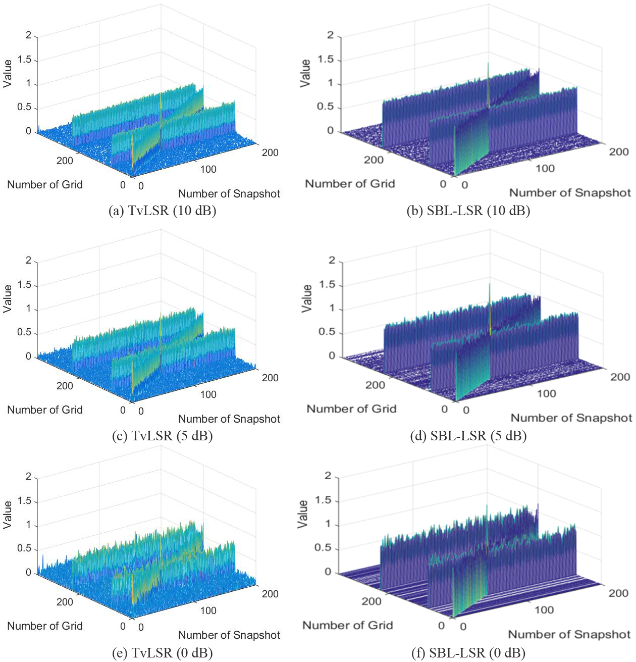
In this simulation, we compared the DOA estimation of the admix sources of TvLSR and SBL-LSR in different SNR. The ULA elements 60, and the number of snapshot 200.
Tracking performance of TvLSR and SBL-LSR in different SNR.
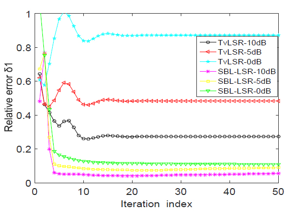
Relative error 1.
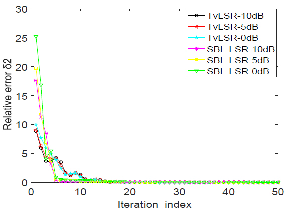
Relative error 2.
Figure 2 shows the tracking performance of TvLSR and SBL-LSR in different SNR for two stationary source and one moving source. And the stationary source is located in the 80th grid and 130th grid, while the moving source moves from 1st to 100th grid over 100 snapshots. Comparing the recovery of low-rank and sparse matrix, the results in Fig. 2 show that the proposed method surpasses TvLSR around the recovery in low SNR which can restore 0 and 1 accurately.
As we can see from Figs 3 and 4, the relative error of this two method drops rapidly until it converges in difference SNR. Where and , with represents the observation matrix without noise, and and represent the th iteration recovery results. This result illustrates that our method is convergent in different SNR. And from Fig. 3, we can see the relative error of SBL-LSR is smaller than TvLSR, which illustrates SBL-LSR more robust to noise than TvLSR.
Onclusion
In this paper, we propose a novel method named as SBL-LSR to estimate DOA of admix source. Comparing with the TvLSR, SBL-LSR has better performance for signal recovery in different SNR. The main reason is that SBL-LSR recovery the low-rank and sparse matrix removing the effect of noise according to the new update parameter , while TvLSR recovery the low-rank and sparse matrix by the observation matrix with noise. But there are some works in the future, such as simplified calculation in SBL-LSR and estimate the source which is not on-grid.
Footnotes
This is derivation of partial factors of Eq. (). Denote , , we can obtain the following two equalities:
Thus far, expectation appeared at Eq. () are presented.
References
1.
HuN.YeZ.XuX. and BaoM., DOA estimation for sparse array via sparse signal reconstruction, Aerospace and Electronic Systems IEEE Transactions on49(2) (2013), 760–773.
2.
HyderM.M. and MahataK., Direction-of-arrival estimation using a mixed l 2,0 norm approximation, IEEE Press (2010).
3.
KimJ.M.LeeO.K. and YeJ.C., Compressive music: Revisiting the link between compressive sensing and array signal processing, IEEE Transactions on Information Theory, 59(9) (2013), 6148–6149.
4.
LeeK.BreslerY. and JungeM., Subspace methods for joint sparse recovery, IEEE Press (2012).
5.
MalioutovD.CetinM. and WillskyA.S., A sparse signal reconstruction perspective for source localization with sensor arrays, IEEE Transactions on Signal Processing53(8) (2003), 3010–3022.
6.
StoicaP.BabuP. and LiJ., Spice: A sparse covariancebased estimation method for array processing, IEEE Transactions on Signal Processing59(2) (2011), 629–638.
7.
ZhengJ. and KavehM., Sparse spatial spectral estimation: A covariance fitting algorithm, performance and regularization, IEEE Transactions on Signal Processing61(11) (2013), 2767–2777.
8.
LinB.LiuJ.XieM. and ZhuJ., Direction-of-arrival tracking via low-rank plus sparse matrix decomposition, IEEE Antennas and Wireless Propagation Letters14 (2015), 1302–1305.
9.
CandesE.J.LiX.MaY. and WrightJ., Robust principal component analysis? Journal of the ACM58(3) (2009), 11.
10.
WrightJ.GaneshA.MinK. and MaY., Compressive principal component pursuit, in: IEEE International Symposium on Information Theory Proceedings, 2012, pp. 1276–1280.
11.
TippingM.E., Sparse bayesian learning and the relevance vector machine, Journal of Machine Learning Research1(3) (2001), 211–244.
12.
WipfD., Non-convex rank minimization via an empirical bayesian approach, arXiv preprint arXiv:1408.2054, 2014.
13.
YuL.SunH.BarbotJ.-P. and ZhengG., Bayesian compressive sensing for cluster structured sparse signals, Signal Processing92(1) (2012), 259–269.
14.
YuL.SunH.ZhengG. and BarbotJ.P., Model based bayesian compressive sensing via local beta process, Signal Processing, 108 (2015), 259–271.
15.
WanH.MaX. and LiX., Variational bayesian learning for removal of sparse impulsive noise from speech signals, Digital Signal Processing73 (2018), 106–116.
16.
BalanA.K.RathodV.MurphyK.P. and WellingM., Bayesian dark knowledge, Advances in Neural Information Processing Systems (2015), 3438–3446.
17.
BabacanS.D.LuessiM.MolinaR. and KatsaggelosA.K., Sparse bayesian methods for low-rank matrix estimation, IEEE Transactions on Signal Processing60(8) (2011), 3964–3977.
18.
HowardW.R., Pattern Recognition and Machine Learning, Springer, 2006.
19.
BealM.J., Variational Algorithms for Approximate Bayesian Inference, University of London United Kingdom, 2003.