High precision Taylor Expansion and Piecewise Calculation Square Root algorithm of microcomputer protection

Abstract

Microcomputer Protection System usually needs to carry on Square Root Operations, such as Newton iterative algorithm, traditional Taylor Expansion algorithm, etc. However, there is not enough high precision to calculate for traditional Square Root Operations. Address to this issue, Taylor Expansion and Piecewise Calculation Square Root algorithm is purposed. In this algorithm, square root algorithm of Taylor Expansion and piecewise calculation are used, and then by successive approximation method the error is reduced. At last, by piecewise calculation the radicand is lessening. Simulation shows that, compared error between uniform segment method and non-uniform segment method, Taylor Expansion and Piecewise Calculation Square Root algorithm has the characters such as high precision and low computation. The precision of this algorithm is high enough to the Microcomputer Protection System, in which there is not more than the error 1.5 $\times$ 10 ${}^{-8}$ .

Keywords

Square root Taylor Expansion partition computation approximation of function

1. Introduction

Embedded microcontroller application system usually needs to carry on Fourier transform to obtain the real and imaginary parts of the ac signal, thus to obtain the effective value, and at this time micro controller must carry on the Square Root operation. This is the prerequisite and basis for protecting logic and other algorithms, so the speed and precision of the square root operation directly affect the performance of the microcomputer protection [1].

Many researchers have spent more time in the square root operation. In [2], Digit-Recurrence Algorithms for Division and Square Root with Limited Precision Primitives is proposed, which is suitable for the low power and high radix implementation. This algorithm is based on the look-up table. The accuracy of the look-up table method is not enough. If we want high precision, we will need more limited memory. Moreover, the accuracy and speed of the look-up table method depends on the length of the table interval and the rationality of the table design. To improve the calculation accuracy, the length of the table should be increased, which makes it necessary to take up more memory [3, 4]. With the development of electronic technology, computer protection hardware has been greatly improved, but existing microcontrollers have very limited memory and CPU speed [8], which contradicts the application of computer protection algorithm. In [5], a radix-16 combined division and square root unit obtained by overlapping two radix-4 stages is proposed, which has fast iteration speed. Newton iterative method has high computational precision, however, the approximate degree of initial value and truth value directly determines the number of iterations and the precision of the calculation. The difficulty lies in the improper selection of initial value, which will increase the number of iterations and take long time [6, 7, 8]. However, the dynamic range of voltage and current in actual measurement is large, and the selection of approximate initial value is more difficult.The fixed initial value is usually selected, which results in a particularly slow convergence at some time. Therefore, there is a lack of an excellent square root algorithm for speed and precision. The traditional Taylor Expansion method requires further processing to meet the accuracy requirements [9, 10, 11, 12, 13]. The accuracy and speed of the Taylor expansion method depends on the length of the table interval and the rationality of the table design. In [14] a fused floating-point multiply/divide/square root unit based on Taylor-series expansion algorithm is proposed, which exhibits a reasonably good area-performance balance. This is a kind of existing Taylor Expansion, whose precision is not high enough. Therefore, high precision Taylor Expansion and Piecewise Calculation Square Root Algorithm of microcomputer protection, which open square algorithm of Taylor Expansion and piecewise calculation are used, and then by successive approximation method the error is reduced.

2. Taylor Expansion and error analysis

In this section, we will analyze the process of Taylor Expansion and its error. Taylor’s formula is a way of approximating a function $f(x)$ with $n$ derivatives at $x=x_{0}$ . At first, we expand the Taylor series and then get the error expression. Then we analyze the relationship between error and $n$ derivatives (between error and $x$ ), we devise the method of reduce the error.

Assume $L=\max(\textit{Re},\textit{Im})$ , $A=\frac{S}{L}$ , so: $I=\sqrt{\textit{Re}^{2}+\textit{Im}^{2}}$ , and then $I=\sqrt{L^{2}+S^{2}}=L\sqrt{1+A^{2}}$ , therefore, the following form of the square operation is:

$\displaystyle I_{1}=L\sqrt{1+A^{2}}$ (1)

where 0 $\leqslant A\leqslant$ 1.

The following method of square operation is based on the Eq. (1).

Assume $x={A^{2}}$ , 0 $\leqslant x\leqslant$ 1, and then Eq. (1) may transform:

$\displaystyle\varphi_{(x)}=I_{1}=(1+x)^{0.5}$ (2)

$\varphi(x)$ will be carried out the Taylor Expansion at $x_{0}=$ 0, then expansion of $f_{(x)}$ is:

$\displaystyle\!\!\!\!\!\!\!\!f_{(x)}=1+\frac{1}{2}x-\frac{1}{8}{x^{2}}+\frac{1% }{16}{x^{3}}-\frac{5}{128}{x^{4}}+\frac{7}{256}{x^{5}}+\ldots+\frac{1*(-1)*(-3% )\ldots(3-2n)}{2^{n}*n!}x^{n}+\ldots$ (3)

The Lagrange remainder of Eq. (3) Tayloy series expansion is typed:

$\displaystyle R_{n}(x)=\frac{f_{(\xi)}^{(n+1)}}{(n+1)!}x^{n+1},\xi\in(0,x)$

The relative error is:

$\displaystyle\varepsilon_{r}(\%)=\frac{\left|f_{(\xi)}^{(n+1)}\right|}{(n+1)!}% *\frac{x^{n+1}}{\sqrt{(1+x)}}*100$ (4)

and,

$\displaystyle\left|f_{(x)}^{(n+1)}\right|=\left|\frac{1\cdot(-1)\cdot(-3)% \ldots(1-2n)}{2^{n+1}*(1+x)^{n+\frac{1}{2}}}\right|$ (5)

(5) Due to $x=A^{2}>$ 0 obviously, $x=$ 0, $\left|f_{(x)}^{(n+1)}\right|$ takes the maximum value, therefore, there is:

$\displaystyle\left|f_{(x)}^{(n+1)}\right|\leqslant\left|\frac{1\cdot(-1)\cdot(% -3)\ldots(1-2n)}{2^{n+1}}\right|$ (6)

Substituting Eq. (6) into Eq. (4)

$\displaystyle\varepsilon_{r}(\%)\leqslant\left|\frac{(-1)\cdot(-3)\ldots(1-2n)% }{2^{n+1}*(n+1)!}\right|*\frac{x^{n+1}}{\sqrt{(1+x)}}*100$ (7)

From Eq. (7), obviously, Eq. (3) Taylor’s expansion’s relative error is decided by $x$ and the number of Taylor Expansion items $n$ .

Figure 1.

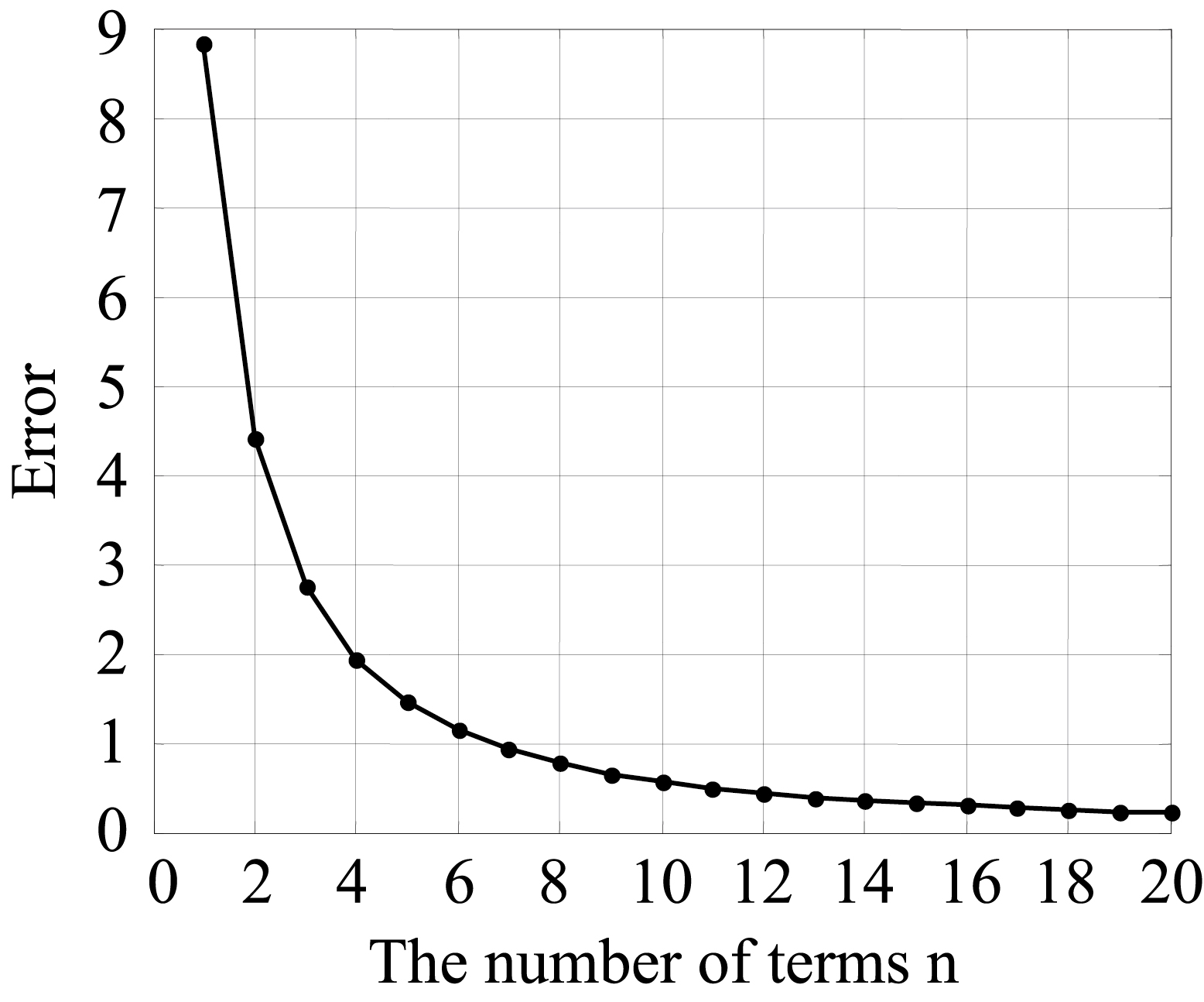
The number of terms $n$ vs. the error.

2.1 The error of Taylor’s expansion and

n

Obviously, the number of terms $n$ is more, the error is smaller as shown in Fig. 1 ( $x=$ 1). We can know that the error is smaller as the bigger $n$ . When $n<$ 5, the relative error decreases sharply with the increase of $n$ . when $n>$ 5, the speed of error declines slowly. The more the number of expansion, the smaller the error, but the greater the amount of computation. Therefore, it is not good to improve the numbers of $n$ in the computational efficiency. When $n<$ 5, the amount of calculation increases little, but the error decreases obviously, so the efficiency is higher; when $n>$ 5, the amount of calculation increases more, but the error decreases less, and the efficiency is lower. For embedded devices, the amount of computation and the speed of computation are still important constraints. Therefore, the number of items $n$ should not exceed 5.

Table 1
The error varies as $x$

$x$	$n=$ 2	$n=$ 3	$n=$ 4	$n=$ 5
1	2.77E $+$ 00	1.65E $+$ 00	1.12E $+$ 00	8.18E $-$ 01
0.5	$-$ 4.89E $-$ 01	1.48E $-$ 01	$-$ 5.09E $-$ 02	1.88E $-$ 02
0.25	$-$ 7.57E $-$ 02	1.16E $-$ 02	$-$ 2.01E $-$ 03	3.75E $-$ 04
0.125	$-$ 1.07E $-$ 02	8.27E $-$ 04	$-$ 7.20E $-$ 05	6.72E $-$ 06
0.1	$-$ 5.61E $-$ 03	3.48E $-$ 04	$-$ 2.43E $-$ 05	1.81E $-$ 06
0.075	$-$ 2.43E $-$ 03	1.13E $-$ 04	$-$ 5.93E $-$ 06	3.32E $-$ 07
0.05	$-$ 7.39E $-$ 04	2.30E $-$ 05	$-$ 8.04E $-$ 07	3.01E $-$ 08
0.01	$-$ 6.18E $-$ 06	3.86E $-$ 08	$-$ 2.70E $-$ 10	2.03E $-$ 12

Figure 2.

$X$ in the interval [0, 1].

Figure 3.

$N$ segment in interval [0, 1].

2.2 The error of Taylor’s expansion and

x

The relative error is approximately proportional to $x^{n+1}$ . When 0 $\leqslant x\leqslant$ 1, the $\frac{x^{n+1}}{\sqrt{(1+x)}}<x^{n+1}$ the Eq. (7) is

$\displaystyle\varepsilon_{r}(\%)\leqslant 100*\left|\frac{(-1)\cdot(-3)\ldots(% 1-2n)}{2^{n+1}*(n+1)!}\right|*x^{n+1}$

From this expression, when $n$ is defined, the relative error is proportional to $x^{n+1}$ . With the decrease of $X$ , the error declines rapidly; otherwise, with the increase of $X$ , the error increases sharply. The relationship between Taylor Expansion relative error and $X$ is shown in Fig. 2. The specific values are shown in Table 1.

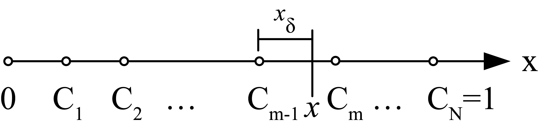
Therefore, $X$ can be reduced in a certain interval as shown in Fig. 3.

Assume that $x$ is in the $m$ th interval, in other word $x\in[C_{m-1},C_{m}]$ , then $x=C_{m-1}+x_{\delta.m}$ where, 0 $\leqslant x_{\delta.m}\leqslant C_{m},C_{m}=C_{m}-C_{m-1}$ , the value $x_{\delta.m}$ is depended on the $N$ segment, usually is smaller than 1.

Then

$\displaystyle I_{1}=(1+x)^{0.5}=(1+C_{m-1}+x_{\delta.m})^{0.5}=\sqrt{1+C_{m-1}% }*\left(1+\frac{x_{\delta.m}}{1+C_{m-1}}\right)^{0.5}$

Assumption: $y=\frac{x_{\delta.m}}{1+C_{m-1}}$ , then:

$\displaystyle I_{1}=(1+x)^{0.5}=\sqrt{1+C_{m-1}}*(1+y)^{0.5}$

Where $\sqrt{1+C_{m-1}}$ , according Eq. (3), we can get the value $(1+y)^{0.5}$ .

Due to $y=\frac{x_{\delta.m}}{1+C_{m-1}}\ll$ 1, then the computational precision would be greatly improved.

Figure 4.

Divides equally $N$ .

3. Segmentation method

In different partition method, the counting error is different. The following concretely analyzes it.

3.1 Divide $x$ into $N$ segments evenly

The easiest way to do this is to divide $x$ in the [0, 1] interval evenly into $N$ segments, as shown in Fig. 4:

Establish $x$ to be in the $m$ cells, namely $x\in[C_{m-1},C_{m}]$ $x=C_{m-1}+x_{\sigma.m}$ 0 $\leqslant x_{\sigma.m}\leqslant C_{m^{\prime}}$ , then $x=C_{m-1}+x_{\delta.m}$ and 0 $\leqslant x_{\delta.m}\leqslant\Delta C_{m},\Delta C_{m}=C_{m}-C_{m-1}\frac{% \delta y}{\delta x}$ , $x_{\delta.m}$ the size depends on the specific segmentation of the $N$ section, generally far less than 1. Then

$\displaystyle I_{1}=(1+x)^{0.5}=(1+C_{m-1}+x_{\delta.m})^{0.5}=\sqrt{1+C_{m-1}% }*\left(1+\frac{x_{\delta.m}}{1+C_{m-1}}\right)^{0.5}$ (8)

Supposing: $y=\frac{x_{\delta.m}}{1+C_{m-1}}$ , then:

$\displaystyle I_{1}=(1+x)^{0.5}=\sqrt{1+C_{m-1}}*(1+y)^{0.5}$ (9)

Then Eq. (9), then

$\displaystyle C_{m-1}=\frac{m-1}{N}\quad y=\frac{x_{\delta.m}}{1+\frac{m-1}{N}% }\quad 0\leqslant x_{\delta.m}\leqslant\frac{1}{N}\quad 0\leqslant y\leqslant% \frac{1}{N}$

When $x$ is evenly divided into the $N=$ 8 sections, in $m$ th sector, $x_{\delta.m}$ maximum value $x_{\delta.(m).\max}$ , $y$ when the maximum value $y_{\delta.(m).\max}$ , as well as computation Taylor launches the square item biggest error $\varepsilon_{r.m}$ as shown in Table 2 according to type Eq. (7).

Table 2

Evenly divided into 8 segments

$m$	$x_{\delta.(m).\max}$	$y_{\delta.(m).\max}$	$\varepsilon_{r.m}$ (%)
1	0.125	0.1250	0.0115
2	0.125	0.1111	0.0081
3	0.125	0.1000	0.0060
4	0.125	0.0909	0.0045
5	0.125	0.0833	0.0035
6	0.125	0.0769	0.0027
7	0.125	0.0714	0.0022
8	0.125	0.0667	0.0018

Figure 5.

Divides equally 8 relative errors and $y$ changing conditions.

As seen in Table 2, the [0, 1] sector is divided into 8 segments evenly, the $y$ maximum value $y_{\max}$ , the maximum error is 0.0115%.

The detailed error and the change of the $y$ when Taylor unfolds into the square is shown in Fig. 2. Obviously, the variation trend of relative error is very similar to that of $y$ ; the maximum relative error between each cell and the maximum value of $y$ are decreasing, the first inter-cell relative error and $y$ maximum are the largest among the individual cells. Because $x=A^{2}$ , therefore, when $x$ is evenly segmented, the segment of $A$ is not uniform, and the segments of $A$ decrease rapidly with the increase of $A$ , in the meanwhile, the maximum value of each cell $y$ decreases rapidly as $A$ increases, so that the relative error is rapidly reduced.

Figure 5, the $x$ -coordinate is $A$ , if the $x$ -coordinate changes to $x$ , the situation is similar. Similarly, if $A$ is evenly divided into $N$ segments, the result is similar to the case where $x$ is evenly segmented, this article no longer analyzes.

3.2 Divide

x

nonuniformly into

N

segments

From the above analysis, it can be seen that the uniform segmentation method is not ideal, because the $y$ maximum of each cell is not uniform, so that the relative error is not uniform, resulting in the largest error is relatively large.

In order to solve the problem of unevenness of each interval after segmentation, the segmentation method should make the maximum value of $y$ in each interval the same, and the maximum error between the individual cells is the same.

Assume that the $x\in[0,1]$ interval is divided into $N$ segments, as shown in Fig. 6.

Establish $x$ to be in the $m$ cells, namely $x\in[C_{m-1},C_{m}]$ , then this sector’s $y$ maximum value $y_{\delta.(m).\max}$ is:

$\displaystyle y_{\delta.(m).\max}=\frac{C_{m}-C_{m-1}}{1+C_{m-1}}$ (10)

and,

$\displaystyle\left\{\begin{array}[]{ll}y_{\delta.(1).\max}=C_{1},&m=1\\ y_{\delta.(m).\max}=\frac{1-C_{N-1}}{1+C_{N-1}},&m=N\end{array}\right.$ (11)

Table 3

Non-uniform divides into eight segments

$m$	$x_{\delta.(m).\max}$	$y_{\delta.(m).\max}$	$\varepsilon_{r.m}$ (%)
1	0.0905	0.0905	0.0044
2	0.0987	0.0905	0.0044
3	0.1076	0.0905	0.0044
4	0.1174	0.0905	0.0044
5	0.1280	0.0905	0.0044
6	0.1396	0.0905	0.0044
7	0.1522	0.0905	0.0044
8	0.1660	0.0905	0.0044

Figure 6.

Non-uniform segmentation schematic drawing.

Figure 7.

Non-uniform divide into eight paragraphs unfold two items error.

Let the maximum value $y_{\delta.(m).\max}$ of each cell $y$ be equal, get the following equations:

$\displaystyle C_{1}=\frac{C_{2}-C_{1}}{1+C_{1}}\quad\frac{C_{2}-C_{1}}{1+C_{1}% }=\frac{C_{3}-C_{2}}{1+C_{2}}\quad\frac{C_{3}-C_{2}}{1+C_{2}}=\frac{C_{4}-C_{3% }}{1+C_{3}}\quad\ldots$ (12) $\displaystyle\frac{C_{N-2}-C_{N-3}}{1+C_{N-3}}=\frac{C_{N-1}-C_{N-2}}{1+C_{N-2% }}\quad\frac{C_{N-1}-C_{N-2}}{1+C_{N-2}}=\frac{1-C_{N-1}}{1+C_{N-1}}$ (13)

Solve the above equations:

$\displaystyle C_{m}=2^{\frac{m}{N}}-1$ (14)

and $m=1,2,\ldots,N$ . At the interval $m$ , $x_{\delta.(m).\max}$ is maximum value of, $y$ the maximum value $y_{\delta.(m).\max}$ , respectively is:

$\displaystyle x_{\delta.(m).\max}=2^{\frac{m}{N}}\left(1-2^{-\frac{1}{N}}\right)$ (15) $\displaystyle y_{\delta.(m).\max}=C_{1}=2^{\frac{1}{N}}-1$ (16)

When $x$ is divided into the eight sections, in the $m$ th interval, $x_{\delta.m}$ maximum value $x_{\delta.(m).\max}$ , the maximum value $y_{\delta.(m).\max}$ , as well as computation Taylor launches the square item biggest error $\varepsilon_{r.m}$ as shown in Table 3 according to type Eq. (7).

As seen in Table 3, the length of $x$ in each cell is increasing as the proportion of $2^{\frac{1}{N}}$ , The maximum value $y_{\delta.(m).\max}$ of $y$ in each cell is the same and the maximum error is the same.When you expand to a square item, the maximum error of each cell is 0.0044%. The detailed error when Taylor Expands $n=$ 2 is shown in Fig. 7.

Figure 8.

Improved algorithm.

Compared with the uniform segmentation method, the non-uniform segmentation method further reduces the maximum value of $y$ , and the $y$ maximum of each cell is equal, thus the maximum relative error decreased by 2.6 times.

4. Algorithm improvement

Note that in the above algorithm, the error is always positive or negative. This is because $x_{\delta.m}$ is a non-negative real number. If $x_{\delta}$ can be positive and negative symmetry, then $x_{\delta}$ will be reduced by half, so the error is greatly reduced.

As shown in Fig. 8, let $x$ be in the $m$ th interval, that is $x\in[C_{m-1},C_{m}]$ ,

Let: $x=C_{m-1}+\frac{1}{2}\Delta C_{m}+x^{\prime}_{\delta.m}$ where, $\Delta C_{m}=C_{m}-C_{m-1}$ , $-\frac{1}{2}\Delta C_{m}\leqslant x^{\prime}_{\delta.m}\leqslant\frac{1}{2}% \Delta C_{m}$ .

Then:

$\displaystyle I_{1}=(1+x)^{0.5}=\sqrt{1+C_{m-1}+\frac{1}{2}\Delta C_{m}}*(1+y^% {\prime})^{0.5}\quad y^{\prime}=\frac{x^{\prime}_{\delta.m}}{1+C_{m-1}+\frac{1% }{2}\Delta C_{m}}$

Compared with the original $x_{\delta.m}$ , the range is 0 $\leqslant x_{\delta.m}\leqslant\Delta C_{m}$ , after improvement $x^{\prime}_{\delta.m}$ , positive and negative symmetry, $x^{\prime}_{\delta.m}\leqslant\frac{1}{2}\Delta C_{m}$ reduced by half.

Error comparison after improvement:

$\displaystyle\frac{\varepsilon_{r}(\%)}{\varepsilon^{\prime}_{r}(\%)}=\frac{% \frac{y^{n+1}}{\sqrt{(1+y)}}}{\frac{y^{\prime n+1}}{\sqrt{(1+y^{\prime})}}}$ (17)

$y^{\prime}=\frac{x^{\prime}_{\delta.m}}{1+C_{m-1}+\frac{1}{2}\Delta C_{m}}$ , $x_{\delta}=\frac{1}{2}\Delta C_{m}+x^{\prime}_{\delta.m}$ brought into the above type, the result is:

$\displaystyle\frac{\varepsilon_{r}(\%)}{\varepsilon^{\prime}_{r}(\%)}=\left(1+% \frac{\frac{1}{2}\Delta C_{m}}{|x^{\prime}_{\delta.m}|}\right)^{n+1}$

Because $|x^{\prime}_{\delta.m}|\leqslant\frac{1}{2}\Delta C_{m}$ , then $\frac{\varepsilon_{r}(\%)}{\varepsilon^{\prime}_{r}(\%)}\geqslant 2^{n+1}$

Therefore, after the algorithm improved, the error is reduced by at least $2^{n+1}$ times. This means that when Taylor is expanded to $n=$ 2, the calculation accuracy is increased by 8 times; when $n=$ 3, the calculation accuracy is improved by 16 times; when $n=$ 5, the calculation accuracy is improved by 64 times. Therefore, this improvement improves the accuracy of the calculation.

5. Algorithm simulation

The above three algorithms are simulated by MATLAB. Taylor Expansion were expanded to 2 ( $n=$ 2). In the simulation, the $x\in[0,1]$ interval is divided into 8 segments, as shown in Fig. 9.

Figure 9.

The [0, 1] Interval is divided into 8 segments.

Figure 10.

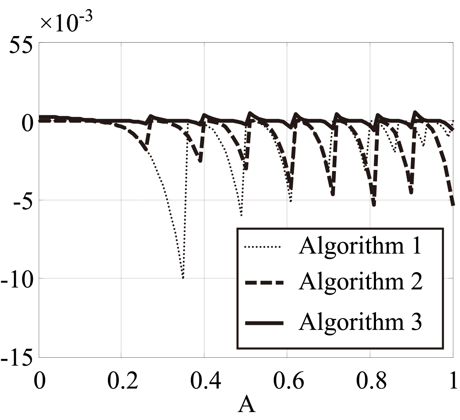
Algorithm simulation result schematic drawing.

The simulation results are shown in Fig. 10. Algorithm 1 is uniform segmentation algorithm, which named Digit-Recurrence Algorithms for Division and Square Root with Limited Precision Primitives [2]. Algorithm 2 is a non-uniform segmentation algorithm, which named a radix-16 combined division and square root unit obtained by overlapping two radix-4 stages [5]. Algorithm 3 is an improved non-uniform segmentation algorithm expands 2 items comparison of three algorithms, which is our improved algorithm.

As can be seen from Fig. 10 and Table 4, the effect of non-uniform segment improvement algorithm is very ideal. Take 8 paragraphs as an example, when it is expanded to 5 times, the error does not exceed 1.5*10 ${}^{-8}$ , this precision is sufficient for the general embedded device.

If it needs to further improve the accuracy of the calculation, it may increase the number of segments to further reduce the $x$ value. See Table 4, if $x$ is reduced to less than 0.01, the error can reach the level of 10 ${}^{-12}$ . After increasing the number of segments, the amount of computation increases little, and only some judgments are added (which cell is the $x$ in).

Table 4

Maximum relative error

Expansion number $n$	Evenly divided	Non-uniformly divided	Non-uniform 8-segment
	into 8 segments	into 8 segments	improved algorithm
2	1.07*10 ${}^{-2}$	4.20*10 ${}^{-2}$	5.33*10 ${}^{-3}$
3	8.26*10 ${}^{-4}$	2.36*10 ${}^{-4}$	1.45*10 ${}^{-5}$
4	7.19*10 ${}^{-5}$	1.49*10 ${}^{-5}$	4.40*10 ${}^{-7}$
5	6.71*10 ${}^{-6}$	1.01*10 ${}^{-6}$	1.43*10 ${}^{-8}$

Table 5

The non-uniform segment ratio is higher than the uniformity of the segmentation accuracy

Expansion number $n$	$k=$ uniform segmentation error/non-uniform segmentation error
2	20.02
3	57.09
4	163.47
5	469.12

Table 6

Non-uniform section improved accuracy is enhanced compared that before improvement

Expansion number $n$	$k=$ error before improvement/improved error
2	7.88
3	16.32
4	33.89
5	70.51

The effect of the improved algorithm is shown in Tables 5 and 6. As can be seen from the table, the more the number of Taylor Expansion items, the higher the accuracy of the algorithm to improve the multiple. Taking $n=$ 5 as an example, the improved algorithm is 70 times higher than that before improvement, which is about 470 times higher than that of the uniform 8 segments algorithm. The effect is obvious. Compared with the reference [15] algorithm, the proposed algorithm can reduce the computational complexity in the case of better accuracy. In reference [16], the author compared the digit-recurrence approach for division and square root to the Newton-Raphson approach. The results of the comparison, in terms of energy consumption and power dissipation, indicate that units based on the digit-recurrence algorithm provide the lowest power solution. In this paper, based on above the Newton-Raphson approach, we prove that the best segment value is perfect for piecewise.

6. Conclusions

For a given function $\varphi_{(x)}$ , a simple approximation function $f(x)$ is used to perform function approximation, and there are many evaluation criteria. For the embedded device, $\varphi(x)-f(x)_{\infty}=\mathop{\max}_{0\leqslant x\leqslant b}\mathop{\max}_% {0\leqslant x\leqslant b}|\varphi(x)-f(x)|$ is usually used, that is, maximum error within 0 $\leqslant x\leqslant b$ rang. In this paper, the error characteristics of $\sqrt{1+x}$ are approximated by the Taylor Expansion method, that is, the error increases sharply with the increase of $x$ . Therefore, in order to reduce the maximum error, the key to the algorithm is to minimize $x$ .

This paper reduces the $x$ by the method of segmentation. The uniform segmentation method will make the maximum value of the number of square meters of each cell uniform, so that the relative error is not uniform, resulting in a greater maximum error. The non-uniform segmentation method has been improved, and the equations are established according to the principle that the number of equations is equal. The value of each segment node is solved. The error of the non-uniform segmentation method is greatly improved, but the error is always positive or negative. Further improve the non-uniform segmentation method, making the error positive and negative symmetry, greatly improving the accuracy of the calculation. MATLAB simulation shows that, in the case of 8 segments, for example, when the power is expanded to 5 times, improved algorithm error is lower than 1.5*10 ${}^{-8}$ . This precision is sufficient for the general embedded device. This paper analyzes in detail the error of the Taylor Expansion partial sum, segmentation method and its error. This part has some reference value for other algorithms using Taylor Expansion partial sum operation, it also has some reference value for other algorithms that use segmentation.

Footnotes

Acknowledgments

This work was supported in part by the following projects: the National Natural Science Foundation of China through the Grants 61571318, the Guangxi Nature Science Fund (2015GXNSFAA139298, 2016GXNSFAA380226), Guangxi Science and Technology Project (AC16380094, 1598008-29), Guangxi Nature Science Fund Key Project (2016GXNSFDA380031), and Guangxi University Science Research Project (ZD 2014146), supported in part by Open Foundation of Guangxi Experiment Center of Information Science LD15030X, Supported by Natural science fund of Guangxi 2015GXNSFAA139298.

References

Tang

Dong

and Zhu

Q.-C.

, Fast SQRT algorithm of microcomputer protection, Power System Protection and Control 38(23) (2010), 1–5.

Ercegovac

M.D.

and Muller

J.M.

, Digit-recurrence algorithms for division and square root with limited precision primitives, in: Conference on Signals, Systems and Computers, 2004.

Wang

Dong

et al., A high-precision square root algorithm for microcomputer protection, Power System Protection and Control 39(19) (2011), 58–62.

Shi

Y.-H.

and Zhang

C.-X.

, The realization of the rapid extraction algorithm on the microcontroller, Computer Technology and Development 24(3) (2007), 30–34.

Nannarelli

, in: IEEE 2011 IEEE 20th Symposium on Computer Arithmetic (ARITH) – Radix-16 Combined Division and Square Root Unit, Tuebingen, Germany (2011.07.25–2011.07.27) 2011, pp. 169–176.

Jiang

H.-W.

Liang

and Liu

J.G.

, The quick square root method of microprocessor, Electronic Science and Technology Nov 15, (2014), 35–36.

Wang

and Zhang

Y.-Y.

, Analysis and Comparison of Microcomputer Protection Algorithms Technology Wind 2013/14, pp. 34–35.

Zhang

J.R.

, Review on the Simulation Algorithms of the Digital Relay ProtectionThe World of Inverters 2016/11, pp. 89–9194.

Xue

C.-X.

, Research on AC Sampling Algorithm for Relay Protection of Microcomputer Relay in Power System . Xi’an University of Electronic Science and Technology, 2012.3.

10.

Zhang

X.-M.

and Li

Y.-X.

, High precision and fast extraction algorithm based on the newton iteration method, Electric Power Automation Equipment (3) (2008).

11.

Chen

L.-Y.

Liang

X.-D.

and Ding

C.-B.

, Based on Look-up table method of fast floating-point Number Square Root Method, Microcomputer Information 25(2–3) (2009), 205–206.

12.

Zhang

L.-P.

and Yang

F.-W.

, The iterative learning algorithm based on Taylor series, Control and Decision (4) (2005), 444–447.

13.

Abrate

Barbero

Cerruti

and Murru

, Periodic representations and rational approximations of square roots, Journal of Approximation Theory 175 (2013).

14.

Ercegovac

M.D.

and Lang

, Division and Square Root: Digit Recurrence Algorithms and Implementations , Kluwer: Boston; 1994.

15.

Kwon

T.J.

and Draper

, Floating-point division and square root using a Taylor-series expansion algorithm, Microelectronics Journal 40 (2009), 1601–1605.

16.

Walczyk

C.J.

Moroz

L.V.

and Cieslinski

J.L.

, Improving the accuracy of the fast inverse square root algorithm, arXiv:1802.06302 [cs.NA], 2018.

High precision Taylor Expansion and Piecewise Calculation Square Root algorithm of microcomputer protection

Abstract

Keywords

1. Introduction

2. Taylor Expansion and error analysis

Table 1 The error varies as x

3.1 Divide x into N segments evenly

Footnotes

Acknowledgments

References

Table 1
The error varies as $x$

3.1 Divide $x$ into $N$ segments evenly