Modeling and simulation of transmembrane ionic transport of cells exposed to magnetic field using the Monte Carlo method

Abstract

This work presents a model for the simulation of plasmatic transmembrane ionic transport that may be exposed to a static gradient magnetic field. The simulation was carried out using the Monte Carlo method to simulate the transmembrane cell transport of five types of ions and obtain observables such as membrane potential, ionic current, and osmotic pressure. To implement the Monte Carlo method, a Hamiltonian was used that includes the contributions of the energy due to the cellular electric field, the electrostatic interaction between the ions, the friction force generated by moving the ion in the center and the contribution given by subduing a cell to a magnetic field gradient. The input parameters to carry out a simulation are the intra and extracellular concentrations of each ionic species, the length of the extracellular medium, the number of Monte Carlo steps (MCS) and the value of the magnetic gradient. The model was validated contrasting it with Gillespie’s algorithm to obtain variations less than 3 % in terms of membrane potential. The Monte Carlo Method combined with the Metropolis algorithm were considered for recreating the stochastic behavior of ion movement.

Keywords

Ion channels membrane potential ionic current magnetic gradient Gillespie algorithm

1. Introduction

To understand the structure and functioning of living organisms, it is essential to know the structure and operation of cells. For this reason, since the end of the 18th century some experimenters raised the need to study transmembrane cell ionic transport [1, 2]. This study started with the identification of the structure of the cell wall [3] and subsequently it was found that a thin layer of oil exhibits a behavior similar to that of a semipermeable membrane and similar to the plasma membrane [4] which allows the construction of physical parameters of the plasma membrane based on the values determined for the oil layer. Additionally, it was established that any substance entering or leaving the cell must be at least soluble in oil [5]. In 1941 it was determined that the membrane is permeable to the ions of K ${}^{+}$ , Cl ${}^{-}$ , Na ${}^{+}$ , Ca ${}^{2+}$ and Mg ${}^{2+}$ [6], and that the knowledge about the transport of these ions is a fundamental aspect to understand different processes of the membrane and of the cell in general. On the other hand, in the field of plant study, transmembrane ionic transport has been analyzed and quantified experimentally using techniques such as radiotracers, external microelectrodes or specific cell-type analyses for transport substrates [6, 7]. However, it is necessary to understand these phenomena from the theoretical point of view and thus, be able to predict their behavior over time or in the presence of disturbances, reason why works including methods of modeling and simulation of the different phenomena that occur in transmembrane cell ionic transport have been carried out.

Regarding the theoretical studies of transmembrane cell ionic transport, analytical advances were proposed initially. One of these studies was conducted by Nernst-Planck (NP) and subsequently modified from the theories of Poisson and Boltzmann. Since the end of the 20th century, with another approach, studies have been carried out using stochastic methods [8] such as the Molecular Dynamics (MD) method with which the total time interval of simulation is a limitation [9]. To extend the simulation times, the Brownian Dynamics (BD) method has been applied, having a lower computational cost compared to the MD method. This improvement was achieved by modeling the process applying a spherical ionic system, an impermeable membrane system and a system of cylindrical pores [10]. On the other hand, Wonpil Im et al. [11] carried out an algorithm to simulate the movement of ions in membrane channels implementing boundary concentration conditions. Recently, Bo et al. [12] simulated the transport for the case of Ca ${}^{2+}$ ion channels activated by voltages and submitted to magnetic fields and temperature changes. They found that the most significant biological changes occur with the exposure to magnetic fields and changes in the channel activation and deactivation. Furthermore, Martinez et al. [13] presented simulations to understand the behavior of the proteins specialized in water transport.

The focus of this work provides a framework to simulate ion permeability to the ions. Using the Monte Carlo (MC) method with the canonical ensemble, a system of biological channels of Na ${}^{+}$ has been modeled in which mobile ions and structural groups are represented as charged hard spheres [14]. Also, hybrid models have been made using the NP equation with a technique known as Local Equilibrium Monte Carlo (LEMC), which is an adaptation of the Grand Canonical Monte Carlo method. Then, NP $+$ LEMC was applied to a system that has two electrolyte deposits, which are separated by a membrane that allows the diffusion of ions through a nanopore [15]. However, in order to experimentally be able to approach the biophysical parameters of the cell membrane, the equipment and processes are quite demanding and expensive. On the other hand, from a computational approach, taking into account stochastic processes, the studies reported using the DB and the MD methods for the study of transmembrane ionic transport, but only specific channels could be simulated and their structure had to be known. On the contrary, using the MC method, a group of channels could be simulated without having to know their structure. It is known that the Monte Carlo method combined with the Metropolis algorithm has shown great efficiency and ease when simulating physical phenomena that lead to a high stochastic behavior [16].

The contribution of this work lies in the integration of various phenomena in transmembrane ionic transport of cells, including the influence of the magnetic field which has been poorly modeled despite the fact that several works are reported experimentally. The few models developed to understand the influence of the magnetic field on this phenomenon generally use deterministic methods, and very little literature is found with the Monte Carlo method. Furthermore, this study included simulation of the movement of the five ions with the highest concentration in the intra and extracellular regions, which is not frequent due to complexity.

For the above reasons, the objective of this work is to propose a model to simulate the process of transmembrane ionic transport and its relationship with variables of interest such as membrane potential, ionic current and osmotic pressure. It also aims to observe the effect on the biophysical parameters mentioned when they have been exposed to a magnetic gradient in the Direct Current (DC).

2. Model description

The model used attempted to include several contributions that force the ions to move through the cellular membrane. These contributions are included in the energy equation (Hamiltonian). Before starting with the description of the Hamiltonian in a more detailed way, the list of parameters used in this work and a brief description of them, including units, is presented in Table 1, These parameters will appear not only in the model, but also in the simulation process.

Table 1
List of parameters included in the work, with their definitions and units

Parameter	Units	Description	Parameter	Units	Description
$[\textit{Ion}]_{e}$	mEq/L	Concentration of the ion in the extracellular medium	$v$	$\mu m/s$	Speed with which the ion moves in the medium
$[\textit{Ion}]_{i}$	mEq/L	Concentration of the ion in the intracellular medium	$\chi_{\bot}$	$m^{3}/kg$	Parallel magnetic susceptibility
$P_{\textit{ion}}$	1/s	Ion permeability	$\chi_{\|\|}$	$m^{3}/kg$	Perpendicular magnetic susceptibility
$\lambda_{D}$	$\mu m$	Debye length	$\Delta\chi$	$m^{3}/kg$	Variation of magnetic susceptibility
$l_{\textit{intra}}$	$\mu m$	Intracellular medium length	$B$	$m T$	Magnetic flux density
$l_{\textit{ext}}$	$\mu m$	Extracellular medium length	$V_{\textit{extra}}$	$\mu m^{3}$	Extracellular volume
$r_{e}$	$\mu m$	Extracellular radius	$V_{\textit{intra}}$	$\mu m^{3}$	Intracellular volume
$r_{i}$	$\mu m$	Intracellular radius	$p$	$J/T$	Magnetic moment of each ion
$\nabla B$	$T/m$	Magnetic Gradient	$z$	–	Valence of each ionic species
$\Delta U$	$m V$	Variation of potential	$e$	$C$	Charge of the electron
$\varrho$	$\mu m$	Radii of each ion	$\pi_{\textit{extra}}$	Pa	Extracellular pressure
$\mu$	$Pa\cdot s$	Kinematic viscosity of the fluid	$\pi_{\textit{intra}}$	Pa	Intracellular pressure

On the other hand, the Hamiltonian that expresses the energy of the system and from which the observables were derived, is shown in Eq. (1). This equation integrates several contributions that are present in transmembrane transport of ions. Four contributions of energy were included depending on the phenomena presented. The integration of these four contributions was developed in this work since, to the researchers’ knowledge, there are no works that contain all these terms including the influence of the external magnetic field. The first term refers to the contribution of the cell own electric field [17]; the second term is due to the electrostatic interaction between the ions [18]; the third term is the contribution due to the friction force that the ions undergo by movement [19]; and the last term is the contribution due to the interaction of the biological system with the energy of the magnetic gradient based on the work of Azanza et al. [20]. In this work, the authors made an experimental and theoretical comparison in neutral networks exposed to the magnetic field

$\displaystyle H=q\cdot\Delta U+k\mathop{\sum}\limits_{[{i,j}]}\frac{q_{i}q_{j}% }{r_{ij}}-6\cdot\pi\cdot\varrho\cdot\mu\cdot\nu\cdot\Delta r-\frac{1}{2}\cdot% \frac{B}{\mu_{0}}\left({\chi_{\bot}+\Delta\chi\cdot\cos^{2}\theta}\right)$ (1)

In the equation, $q$ is the value of charge of each ion; $\Delta U$ is the variation of the potential calculated according to Eq. (4); $k$ is the constant of proportionality that has a value of 8.99 $\cdot$ 10 ${}^{9}$ N $\cdot$ $m^{2}\cdot$ C ${}^{-2}$ ; $r_{ij}$ is the distance between each pair of ions; $\varrho$ is the radii of each ion; $\mu$ is the kinematic viscosity of the fluid (value of olive oil 0.090 $Pa\cdot s$ ); $v$ is the speed with which the ion moves in the medium calculated according to Eq. (2) [21] which will be presented at the end of this paragraph.; $\Delta r$ is the change in the position of the ion; $B$ is the magnetic flux density in a linear medium which is in the same direction of the electric field; $\mu_{o}$ is the magnetic permeability in vacuum $4\pi\cdot$ 10 ${}^{-7}$ T $\cdot$ m $\cdot$ A ${}^{-1}$ ; $\Delta\chi$ is the variation of the magnetic susceptibility; $\chi_{\bot}$ is the magnetic susceptibility perpendicular to the ion channel, and $\chi_{||}$ is the magnetic susceptibility parallel to the ion channel; lastly, $\theta$ is the angle that is formed between the longitudinal axis of each channel to the line that intercepts the position of the particle [20].

2.1 Importante: Ver comentario

$\displaystyle\vspace*{-0.5cm}\nu=\frac{2}{g}\frac{r^{2}\cdot g\cdot\left({\rho% _{i}-\rho_{f}}\right)}{\mu}$ (2)

in which $g$ is the gravitational acceleration with a value of 9.80 $m\cdot^{-2}$ ; $\rho_{i}$ is the density of each ionic species, and $\rho_{f}$ is the density of the solvent ( $\rho_{f}=$ 0.916 kg $\cdot$ L ${}^{-1}$ ); $\rho_{f?}?$ is assumed to be the density of olive oil, according to Rodi et al. [22]. The importance of this density is considered due to the fact that the transmembrane transport occurs in a liquid (intra and extracellular liquid) using Eq. (2) to calculate the speed of the ions movement. This speed depends on viscosity and density

3. Simulation process

Once the model was built and all the contributions were considered, the required parameters were determined and identified and the simulation process was developed divided into three main parts: sample construction, ion movement and calculation of observables. To visualize the simulations, according to computational time and the Monte Carlo methodology, the following assumptions were considered

1.
The cell was considered as an isolated part of the rest of the organism.
2.
The cell was considered to be spherical in shape, with a cross section of 5 Å.
3.
The channel was considered to have a cylindrical structure.
4.
Although in the real experiment several ions could be transported at the same time, only one ion could be moved at each time because of the essence of the model and Monte Carlo simulations.

All simulation processes are represented in Fig. 1, which contains a flow diagram. This figure shows stages such as sample construction, Hamiltonian construction, ion movement including the Monte Carlo Method and the Metropolis Algorithm, and finally, the observable calculation (resting potential unaffected and affected by the magnetic field, and osmotic pressure)

Figure 1.
Flow diagram where all the stages of the simulation process are included.

Each stage of the simulation process is described below.
3.1 Sample construction

As mentioned above, the model used an isolated spherical cell with the nucleus inside. The extracellular radius ( $r_{e}=$ 5.000 $\mu m$ ) was used for this model taken from the work presented by Socorro et al. [18] that suggested this value for a cell subjected to a magnetic field. In addition, the intracellular radius ( $r_{i}=$ 4.992 $\mu m$ ) was defined by taking the membrane thickness as 8 nm. Two cross-section cuts were made equidistant from the sphere equator with a separation ( $s$ ) of 5 Å between them, generating a ribbon-like section similar to that surrounding the cell (Fig. 2). This section of the membrane is waterproof and contains 278 channels, numbers determined according to geometric and morphological parameters (see Annex 1: calculation of number of channels and number of ions). Passive channels were assumed, considered as non-deformable pores with a cylindrical structure with an average external radius of 3.0 Å that will remain activated throughout the simulation time, which implicitly suggested that they are not voltage-controlled channels. The location of these channels on the membrane, according to the species and the position, was carried out randomly and they were distributed in the following proportions: 91.83% cation channels (255) with internal radii of: 1.17 Å for Na ${}^{+}$ , 0.9 Å for Mg ${}^{2+}$ , 1.55 Å for K ${}^{+}$ , and 1.15 Å for Ca ${}^{2+}$ , and 8.17% are channels of Cl ${}^{-}$ (28) with internal radii of 1.70 Å. Spherical [23] and dehydrated ions were assumed. The calculation of the number of ions and the number of channels is explained in Annex I. The ions K ${}^{+}$ , Na ${}^{+}$ , Mg ${}^{2+}$ , Ca ${}^{2+}$ $y$ Cl ${}^{-}$ are considered in this work since they are the ions found in a higher concentration in the cells [24].

The intracellular and extracellular medium were subdivided into square unit cells side of 5.0 Å. These spaces have limits that determine how far the model perceives the ions. The intracellular compartment has a fixed depth ( $l_{\textit{intra}}$ ) and the extracellular one is variable. The length ( $l_{\textit{ext}}$ ) was determined from the external surface of the cell to the outer limit that meets the relationship between total cell volumes according to the literature [24], $V_{\textit{extra}}=$ 0.6 $\cdot$ $V_{\textit{intra}}$ with $\lambda_{D}\leqslant l_{\textit{ext}}\leqslant$ 17.0 $\mu m$ ( $\lambda_{D}$ corresponds to the Debye length). The value of $\lambda_{D}$ was dependent on the concentrations, therefore, for normal physiological conditions $\lambda_{D}=$ 5.0 nm.

Figure 2.

Structural detail of the modeled cell segment. Ions and channels of potassium (green), magnesium (pink), sodium (red), chloride (cyan) and calcium (dark blue).

Regarding the temporal parameter, the equivalence of an MCS at 10 ps was taken based on the DM studies [25].

3.2 Ion movement

Ionic transmembrane transport is a stochastic phenomenon. Like many natural phenomena, ion movement does not follow a deterministic behavior and a specific sequence. For this reason, the Monte Carlo method, combined with the Metropolis algorithm, which is based on the probability of occurrence of some event, is an adequate method to simulate this ionic movement. After deciding to use the Monte Carlo method, the ion movement was defined according to established biological conditions [26], that is to say, in a cell the ions were highly diluted in the extracellular and intracellular medium, the movement of the ions went from the site of higher concentration to lower concentration and, furthermore, the channels were active during the simulation . Concentrations in the intracellular and extracellular medium were calculated to estimate the value of the membrane potential for each MCS and, from this value, to calculate its contribution to the Hamiltonian and, ultimately, to determine the displacement for each ion generating a movement by concentration gradient. To determine the movement of ions in both media, the fact that only one ion can be located for each unit cell and the electrostatic interactions of the ion selected with the ions around it were considered (first, second, third, fourth up to the nth neighbor). Each attempt to move an ion equaled one MCS. The membrane potential and the concentration for each ion type were calculated by running each MCS:

1.
A position $r_{1}$ was chosen in which the movement was started at random according to the Metropolis algorithm [27] and subsequently, the ion located there was identified and its energy $E_{1}$ was calculated Eq. (1).
2.
The probability of movement was calculated based on the electrostatic interactions with the other ions to determine the new position $r_{2}$ and the energy $E_{2}$ in that new position was also calculated.
3.
The energy values were compared and, if $E_{2}<E_{1}$ , the movement of the ion was accepted fulfilling the selectivity conditions.
4.
If $E_{2}>E_{1}$ , the value of a probability $w$ was calculated,

$\displaystyle w=\textit{exp}\left({-\Delta E/k_{B}T}\right)$ (3)

and a random number ( $t$ ) between 0 and 1 was generated. If $t<w$ , the movement was accepted. But, on the contrary, if $t>w$ it was necessary to go back to step 1.
5.
The stop condition was defined by the scope of the amount of MCS established. This was an input parameter of the simulation.

The validation of the implemented model was based on the comparison of the model with Gillespie’s algorithm. This method was selected due to its constant use in chemical or biochemical systems and because it is additionally useful to simulate reactions within cells, as it is the most appropriate when this type of processes occurs in biological systems [28]. This algorithm consists in generating a statistically correct trajectory (possible solution) of a stochastic equation. The algorithms are framed by a density function that determines the probability of an event or reaction occurring.
3.3 Observables calculation

As mentioned before, using the model and simulation process, it is possible to calculate observables as ionic concentration, resting potential without the effect of the magnetic field, which represents the potential difference that exists between the inside and the outside of the cell and generating the action potentials also known as electrical impulse, which are a wave of electrical discharge that travels along the cell membrane that modifies its distribution of electrical charge and other electrical signals by activating the flow of transmembrane ions [29]. This potential was determined from Eq. (4):

$\displaystyle V_{m}=\pm\frac{\textit{RT}}{F}\textit{Ln}\!\!\left[\frac{P_{K^{+% }}[K^{+}]_{e}\!+\!P_{\text{Na}}\!+\![\text{Na}^{+}]_{e}\!+\!P_{\text{Cl}^{-}}[% \text{Cl}^{-}]_{i}\!+\!P_{\text{Ca}^{2+}}[\text{Ca}^{2+}]_{e}\!+\!P_{\text{Mg}% ^{2+}}\!+\![\text{Mg}^{2+}]_{e}}{P_{K^{+}}[K^{+}]_{i}\!+\!P_{\text{Na}}\!+\![% \text{Na}^{+}]_{i}\!+\!P_{\text{Cl}^{-}}[\text{Cl}^{-}]_{e}\!+\!P_{\text{Ca}^{% 2+}}[\text{Ca}^{2+}]_{i}\!+\!P_{\text{Mg}^{2+}}\!+\![\text{Mg}^{2+}]_{i}}\right]$ (4)

where: $R$ is the universal gas constant; $T$ is the absolute temperature of the system which, in this case, is 308.15 K; $F$ is the Faraday constant 96 485.336 5 $C\cdot\textit{mol}^{-1}$ ; $P_{K^{+}}$ , $P_{\text{Na}^{+}}$ , $P_{\text{Cl}^{-}}$ , $P_{\text{Ca}^{2+}}yP_{\text{Mg}^{2+}}$ are the permeabilities of each type of ion $P_{K^{+}}$ : $P_{\text{Cl}^{-}}$ : $P_{\text{Na}^{+}}$ : $P_{\text{Mg}^{2+}}$ : $P_{\text{Ca}^{2+}}=\left({1:0.45:0.04:0.09:0.11}\right)$ ; the concentrations of each type of ion are $\left[{K^{+}}\right]$ , $\left[{\text{Na}^{+}}\right]$ , $\left[{\text{Cl}^{-}}\right]$ , $\left[{\text{Ca}^{2+}}\right]y\left[{\text{Mg}^{2+}}\right]$ and the subscripts $i$ and $e$ refer to the intracellular and extracellular medium, respectively.

On the other hand, resting potential with the effect of the magnetic field gradient was calculated using to the Eq. (5)

$\displaystyle V_{m}=\pm\frac{\textit{RT}}{F}\textit{Ln}\left[\frac{P_{K^{+}}[K% ^{+}]_{e}+P_{\text{Na}}+[\text{Na}^{+}]_{e}+P_{\text{Cl}^{-}}[\text{Cl}^{-}]_{% i}+P_{\text{Ca}^{2+}}[\text{Ca}^{2+}]_{e}+P_{\text{Mg}^{2+}}+[\text{Mg}^{2+}]_% {e}}{P_{K^{+}}[K^{+}]_{i}+P_{\text{Na}}+[\text{Na}^{+}]_{i}+P_{\text{Cl}^{-}}[% \text{Cl}^{-}]_{e}+P_{\text{Ca}^{2+}}[\text{Ca}^{2+}]_{i}+P_{\text{Mg}^{2+}}+[% \text{Mg}^{2+}]_{i}}\right]+\sum\frac{p}{ze}\left|\frac{dB}{dl}\right|L$ (5)

where $e$ is the charge of the electron; $z$ is the valence of each ionic species; $p$ is the magnetic moment of each ion, defined as follows: $p\text{Na}^{+}=$ 2.22 $\cdot\mu_{n}$ , $pK^{+}=$ 0.390 $\cdot\mu_{n}$ , $p\text{Cl}^{-}=$ 0.820 $\cdot\mu_{n}$ , $p\text{Ca}^{2+}=$ 0.00145 $\cdot\mu_{n}$ y $p\text{Mg}^{2+}=$ 1.20 $\cdot\mu_{n}$ con $\mu_{n}=$ 5.05 $\times$ 10 ${}^{-27}$ $J\cdot T^{-1}$ , which is deduced from the relation $\mu_{B}/\mu_{n}\simeq$ 18.36 with $\mu_{B}=$ 9.274 009 68 $\times$ 10 ${}^{-24}$ $J\cdot T^{-1}$ and $dB/dL$ magnetic gradient. The expression of the gradient depends on the geometric shape of the magnetic field generator. In this case, two flat cross-section magnets, magnetized through the thickness and positioned concurrently [30] at a distance $x=$ 80 $\mu m,$ were used with the cell located between them. This parameter was calculated using the following expression Eq. (6),

$\displaystyle\left({2\sqrt{2}\mu_{0}M_{R}}\right)/\pi x$ (6)

taking $\mu_{0}M_{R}$ in an approximate interval of (1.0–1.2) T, $M_{R}$ is the remnant magnetization. The basis for choosing the magnetic gradient values with which the simulations were carried out were assumed according to the results of the study of passive magnetic sources carried out by Torres et al. [31].

Osmotic pressure is the difference between extra and intracellular pressure and was calculated as follows:

$\displaystyle\Delta\pi=\pi_{\textit{extra}}-\pi_{\textit{intra}}$

where $\pi_{\textit{extra}}=\left[\textit{Ion}\right]_{\textit{extra}}R\cdot T$ and $\pi_{\textit{intra}}=\left[\textit{Ion}\right]_{\textit{intra}}R\cdot T$ with $R$ as a universal gas constant 8.314472 $\left({J/\left({\textit{mol}\cdot K}\right)}\right)$ and $T$ as temperature 308.15 K. This temperature is the temperature of the cells [24].

4. Results

4.1 Membrane potential

Figure 3 shows the comparison of the membrane potential as a function of time using the Monte Carlo method and Gillespie’s algorithm. As can be observed, the same trend is maintained for both, which shows that the implemented model adapts to Gillespie’s algorithm and, furthermore, it can be seen that the variations barely reached a maximum value of 3%. The differences can be attributed to the way the Monte Carlo steps were calculated in Gillespie’s algorithm since, every time a Monte Carlo step was fulfilled, the difference between the steps was recalculated. The constant fluctuations of the membrane potential are due to the constant transmembrane movement of the ions. To define the moment in which the concentrations were going to change direction, a limit for the variation in the concentration was calculated to preserve the homeostatic equilibrium. The limit of the variations in the concentrations were defined randomly at the beginning of the simulations in order to resemble the stochastic behavior that occurs in nature. This type of behavior was previously reported by Ramírez et al. [32] who studied conical pores covered with amphoteric lysine groups.

Figure 3.

Membrane potential as validation of the model proposed with Monte Carlo using Gillespie’s algorithm.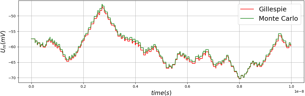

A model was obtained that allows simulating the transport of five types of ions through passive channels whose activation or inactivation status is independent on the intracellular voltage values. As proposed in the methodology, the model allows observing the behavior of the membrane potential (Fig. 3) and the ionic concentration (Fig. 4).

4.2 Ionic concentration of each species

Figure 4 shows the behavior of ionic concentration for five species as a function of time. To carry out the simulations, the cell was considered to be initially in electrochemical equilibrium. The concentrations of Ca ${}^{2+}$ and Na ${}^{+}$ ions had less variation compared to those of the $K^{+}$ , Cl ${}^{-}$ and Mg ${}^{2+}$ ions. The variations in concentrations for Ca ${}^{2+}$ ions was 1.2 $\times$ 10 ${}^{-5}$ mEq/L; for Na ${}^{+}$ ions was 0.35 mEq/L; for Cl ${}^{-}$ ions was 2.4 mEq/L; for Mg ${}^{2+}$ ions was 2.4 mEq/L; and for $K^{+}$ ions was 45 mEq/L. Comparing the variations of $K^{+}$ , Cl ${}^{-}$ and Mg ${}^{2+}$ ions, it was evident that for $K^{+}$ ions the variation was much wider which is due to the fact that for $K^{+}$ the number of ions was 31 836 and their movement by concentration gradient was carried out from the intracellular to the extracellular medium, which means that many more ions moved for changes in concentration to occur. For the Cl ${}^{-}$ ions the amplitude in the fluctuations was due to the fact that, by concentration gradient, the movement of this type of ions was carried out from the extracellular to the intracellular medium and, for the intracellular concentration to change, approximately ten times the number of Ca ${}^{2+}$ ions must have entered and left constantly. For Mg ${}^{2+}$ ions, the amplitude in the variations of the concentration is due to the fact that it was the second type of ion with more number of ions in the intracellular medium and, therefore, they must have moved approximately seven times the number Ca ${}^{2+}$ ions for changes in intracellular concentration to occur. To define the point where concentrations would change direction, it was required to identify the limit of concentration variation. To maintain homeostatic equilibrium, this limit was initially defined randomly in order to resemble the stochastic behavior that occured in this kind of phenomenon. This same behavior has been reported previously by Ramírez et al. [32] who studied conical pores covered by of lysine amorphous groups. Also, using the molecular dynamics for the Gramicidin A channel, the random behavior is shown in the ionic current which changes according to the ionic concentrations [25].

Figure 4.

Behavior of the intracellular concentration of each ionic species over time.

4.3 Osmotic pressure

Figure 5.

Osmotic pressure in function time.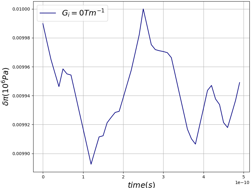

Figure 5 shows the osmotic pressure as a function of time. Fluctuations can be observed, that correspond to changes in the concentrations of the different ionic species. Biologically, these changes in the osmotic pressure generated changes in the membrane permeability as reported by Stange et al. [18]. Additionally, these variations accelerated the chemical processes related to the hydrolysis.

5. Perspectives

The addition of other geometric shapes is considered for the magnetic field generating source. Also, not just a section of the cross section of the cell, but the whole cell can be taken. In addition, a process that allows showing the trajectory that the particles follow in their movement must be considered which will allow glimpsing possible effects that the magnetic gradient has on the transmembrane ionic transport, which requires significant computational time and the implementation of an advanced algorithm.

6. Conclusions

•

The Monte Carlo Method combined with the Metropolis algorithm were considered to recreate the stochastic behavior of ionic movement showing that, using the Monte Carlo method, it is possible to model ionic transport due to its stochastic nature. Furthermore, the proposed model was validated with the evaluation of Gillespie’s algorithm.

•

To develop the model of transmembrane ion transport, cellular dimensions ( $r_{i}$ y $r_{c}$ ) were taken into account. In addition, five ion species ( $K^{+}$ , Na ${}^{+}$ , Cl ${}^{-}$ , Mg ${}^{2+}$ and Ca ${}^{2+}$ ) were considered. Ions were highly diluted and the energy contributions considered four terms: electric field, the ion interaction, friction force and influence of the external magnetic field.

Footnotes

Acknowledgments

The authors would like to thank La Facultad de Ciencias Exactas y Naturales at the Universidad Nacional de Colombia- Sede Manizales, for the economic support by means of the postgraduate students’ scholarship. Also, to the “Desarrollo de un sistema automático de tratamiento magnético de semillas asociado a un entorno integrado de simulaciones y optimización del diseño de experimentos” project developed by Universidad de Caldas and Universidad Nacional de Colombia- Sede Manizales.

Annex 1: Calculation of number of channels and number of ions

•

The average density of the channels was defined as proposed by Ferrero et al. [24]. The cell surface section area that was taken into account for the simulation is $S_{\textit{total}}=$ 1.57 $\times$ 10 ${}^{-13}$ m ${}^{2}$ , was determined based on the cell radii (5.0 $\mu m$ ). Then, the effective area of the channels was assumed as $S_{\textit{total}}$ /2000, so $S_{\textit{channels}}=$ 7.85 $\times$ 10 ${}^{-17}$ $m^{2}$ and the average external area of the channels was $A_{\textit{channel}}=$ 2.83 $\times$ 10 ${}^{-19}$ m ${}^{2}$ , being the number of channels $N_{\textit{channel}}=S_{\textit{channels}}/A_{\textit{channel}}=$ 278.

•

The number of ions of each species in the intracellular and extracellular medium was determined as follows:

$\displaystyle N^{\circ}\textit{ions}_{\textit{species}}^{\textit{medium}}=V_{% \textit{medium}}\ast\left[\textit{Ion}\right]_{\textit{medium}}$

where $V_{\textit{medium}}$ is the volume of each of the intracellular and extracellular compartments and $\left[\textit{Ion}\right]_{\textit{medium}}$ is the concentration of each ionic species in $\textit{iones}\cdot\mu\cdot m^{-3}$ . To know the total number of ions in each medium, the ionic species of each medium were added.

References

Fertig

Mádai

Valiskó

and Boda

, Simulating ion transport with the NP LEMC Method. applications to ion channels and nanopores, Hungarian Journal of Industry and Chemistry 45 (2017), 73–84.

Galland

and Pazur

, Magnetoreception in plants, Journal of Plant Research 118 (2005), 371–389.

Quincke

, Ueber periodische Ausbreitung an Flüssigkeitsoberflächen und dadurch hervorgerufene Bewegungserscheinungen, Annalen Der Physik Und Chemie 271 (1888), 580–642.

Davenport

C.B.

, The Cell Outlines of general anatomy and physiology, Science 5 (1897), 111–113.

Gorter

and Grendel

, On bimolecular layers of lipoids on the chromocytes of the blood, J Exp Med 41 (1925), 439–443.

Brooks

S.C.

, The permeability of living cells, Science 100 (1944), 30–31.

Geisler

Wang

and Zhu

, Auxin transport during root gravitropism: transporters and techniques, Plant Biol 16(Suppl 1) (2014), 50–57.

McCormick

D.A.

, Membrane potential and action potential, Fundamental Neuroscience (2013), 93–116. doi: 101016.

Klepeis

J.L.

Lindorff-Larsen

Dror

R.O.

and Shaw

D.E.

, Long-timescale molecular dynamics simulations of protein structure and function, Current Opinion in Structural Biology, 19 (2009), 120–127.

10.

and Roux

, Brownian dynamics simulations of ions channels: A general treatment of electrostatic reaction fields for molecular pores of arbitrary geometry, The Journal of Chemical Physics 115 (2001), 4850–4861.

11.

Seefeld

and Roux

, A grand canonical monte carlo-brownian dynamics algorithm for simulating ion channels, Biophysical Journal 79 (2000), 788–801.

12.

Guo

Yang

Wang

Tang

Zeng

and Gong

, Numerical study of voltage-gated ca2 transport irradiated by terahertz electromagnetic wave, IEEE Access 8 (2020), 10305–10315.

13.

Zhao

Xia

Van Doorsselaere

Keppens

and Gan

, Forward Modeling of SDO/AIA and X-Ray Emission from a Simulated Flux Rope Ejection, The Astrophysical Journal 872 (2019), 190.

14.

Boda

Busath

D.D.

Eisenberg

Henderson

and Nonner

, Monte Carlo simulations of ion selectivity in a biological Na channel: Charge-space competition, Phys Chem Chem Phys 4 (2002), 5154–5160.

15.

Monte-Carlo Simulation of the Ionic Transport of Electrolyte Solutions at High Concentrations Based on the Pseudo-Lattice Model, ECS Meeting Abstracts, (2016).

16.

Morgan

B.J.

, Lattice-geometry effects in garnet solid electrolytes: A lattice-gas Monte Carlo simulation study, R Soc Open Sci 4 (2017), 170824.

17.

Reina

F.G.

Pascual

L.A.

and Fundora

I.A.

, Influence of a stationary magnetic field on water relations in lettuce seeds. Part II: Experimental results, Bioelectromagnetics 22 (2001), 596–602.

18.

Socorro

and García

, Simulation of magnetic field effect on a seed embryo cell, International Agrophysics 26 (2012), 167–173.

19.

Rodi

P.M.

Cabeza

M.S.

and Gennaro

A.M.

, Detergent solubilization of bovine erythrocytes. Comparison between the insoluble material and the intact membrane, Biophys Chem 122 (2006), 114–122.

20.

Azanza

M.J.

Blott

B.H.

del Moral

and Peg

M.T.

, Measurement of the red blood cell membrane magnetic susceptibility, Bioelectrochemistry and Bioenergetics 30 (1993), 43–53.

21.

Feng

Z.-G.

, A correlation of the drag force coefficient on a sphere with interface slip at low and intermediate reynolds numbers, Journal of Dispersion Science and Technology 31 (2010), 968–974.

22.

Rodi

P.M.

Trucco

V.M.

and Gennaro

A.M.

, Factors determining detergent resistance of erythrocyte membranes, Biophys Chem 135 (2008), 14–18.

23.

Maffeo

Bhattacharya

Yoo

Wells

and Aksimentiev

, Modeling and simulation of ion channels, Chem Rev 112 (2012), 6250–6284.

24.

Corral

J.M.F.

y. de Loma-Osorio

J.M.F.

Rodríguez

J.S.

and Vives

A.A.

, BIOELECTRÓNICA. SEÑALES BIOELÉCTRICAS, Ed. Univ. Politéc. Valencia, 1994.

25.

Aponte

C.A.

Munoz

J.D.

and Fayad

, Simulación por dinámica browniana del transporte ionico a través del canal gramicidina a, Revista Colombiana de Física, 38 (2006).

26.

Mujumdar

M.P.

, Monte Carlo simulations of ionic channel selectivity, Comput Appl Biosci 7 (1991), 359–364.

27.

Pang

T.D.

, The Metropolis algorithm, An Introduction to Quantum Monte Carlo Methods, (2016).

28.

Yates

C.A.

and Klingbeil

, Recycling random numbers in the stochastic simulation algorithm, The Journal of Chemical Physics 138 (2013), 094103, doi: 10.1063/1.4792207.

29.

General Biophysics, (1983).

30.

Zablotskii

Polyakova

Lunov

and Dejneka

, How a high-gradient magnetic field could affect cell life, Sci Rep 6 (2016), 37407.

31.

Torres

Hincapie

and Gilart

, Characterization of magnetic flux density in passive sources used in magnetic stimulation, J Magn Magn Mater 449 (2018), 366–371.

32.

Ramirez

Gomez

Ali

Ensinger

and Mafe

, Net currents obtained from zero-average potentials in single amphoteric nanopores, Electrochem Commun 31 (2013), 137–140.