Application analysis of highway traffic accident risk model based on geographically weighted negative binomial regression

Abstract

The traditional generalized linear model (GLM) can not effectively analyze discrete road traffic accidents when analyzing road traffic accidents with spatial dependence and heterogeneity. Therefore, a risk analysis method of highway traffic accidents based on geographically weighted negative binomial regression model (GWNBR) is proposed. Using geographical weighted regression (GWR) model and negative binomial regression (NB) model, this paper makes a comparative analysis of highway traffic accidents in Xi’an, including local spatial geographical weighted Poisson regression (GWPR) model and two geographical weighted negative binomial regression (GWNBRg and GWNBR) models. The corresponding model bandwidth is determined, and the performance of the model is compared based on the data of traffic environment, road characteristics, crowd characteristics and road alignment. The experimental results show that compared with the single NB model, the proposed model can effectively reduce the interference of the spatial nonstationarity of the data, and can effectively extract the risk factors affecting the accident. The coefficients of GWNBRg model and GWNBR model are positive, which are better than GLM in the mean and likelihood of the residuals. The spatial autocorrelation of the residuals is significantly reduced, and the significance level is 5%, which reduces the spatial heterogeneity of the data. The over dispersion parameter value of GWNBRg model shows a downward trend from southwest to northeast in space, which can effectively reflect the spatial relationship between traffic flow and accident rate, indicating that GWNBR model has a good effect in traffic accident risk analysis of super discrete highway. Therefore, the application of geographical weighted negative binomial regression to highway traffic accident risk prediction has a good application effect, and can effectively reduce the probability of accidents as safety prevention and early warning.

Keywords

Geographic weighted model negative binomial regression road traffic accidents traffic accident risk analysis generalized linear model over discretization

1. Introduction

The traffic environment and road characteristics of the road lead to the potential danger of the road and the frequent occurrence of traffic accidents [1]. The highway drives the regional economic development and attracts more traffic. However, the continuous increase of vehicles under the existing road conditions leads to the increase in the number of highway accidents. Different traffic environments also affect the rescue difficulty of traffic accidents. The occurrence of road traffic accidents is random, and there is spatial autocorrelation between the complex environment of the accident and the main causes of the accident [2]. In addition to spatial autocorrelation, accidents are also affected by spatial heterogeneity. Spatial heterogeneity can define spatial related factors, that is, the structural relationship of regional continuous change, which is systematically changed between regions [3]. In order to improve highway traffic safety and identify highway traffic accident risk black spots, it is of great significance to establish a highway accident risk analysis model.

How to identify the road accident risk, effectively establish the road traffic accident risk analysis model, and more accurately analyze, study and judge the road accident risk has attracted the extensive attention of scholars in relevant fields. At present, experts and scholars in related fields have carried out many researches on traffic accident analysis and prediction methods. For example, Duan et al. [4] introduced Pearson coefficient to analyze the correlation between IHSDM predicted accident results and section AADT and section length. The predicted results are quite different from the actual results. Zhang et al. [5] proposed a solution algorithm based on k-shortest path. The model only considers the impact of saturation on traffic accidents, but does not consider factors such as road geometric characteristics and traffic composition. Considering the characteristics of traffic accidents and time series, Ma et al. [6] applied Markov chain algorithm to accident dynamic prediction, the results show that this method can effectively correct the relative error and has a good early warning effect for the randomness and fuzziness of accidents, but its application effect is large, which is limited by the timeliness of data information.

Aiming at the special constraints of highway traffic accidents, the negative binomial distribution model is creatively integrated into the geographically weighted regression model, and a traffic accident risk analysis method based on GWNBR model is proposed. Based on Xi’an Highway traffic accident database, a geographically weighted negative binomial regression model is established for analysis, which explains the effect of accident influencing factors on traffic accidents in special environment, and provides a basis for the interdependence between highway accidents and accident risk black spots.

2. Road traffic accident risk analysis method based on GWNBR model

2.1 Negative binomial distribution model

The negative binomial (NB) distribution is a statistically discrete probability distribution [7]. Because the NB distribution is improved on the basis of Poisson distribution, the study of NB distribution should begin with the derivation of Poisson regression formula. The distribution function of Poisson regression is:

$\displaystyle X({l_{n}})=\frac{\gamma_{n}^{l_{n}}\exp({-\gamma_{n}})}{l_{n}!}$ (1)

In Eq. (1), $X({l_{n}})$ is the probability of $l$ accidents occurring on road section $n$ , then the expectation and variance of Poisson regression distribution function and the relationship between them are expressed as:

$\displaystyle\gamma_{n}=C_{n}$ (2)

In Eq. (2), $\gamma_{n}$ is the expected number of accidents occurring on road section $n$ , and $C_{n}$ is the variance of the number of accidents occurring on road $n$ . The form of $\gamma_{n}$ expressed by the accident influencing factor function is:

$\displaystyle\ln\gamma_{n}=\ln({D_{n}+G_{n}})+\mu_{n}$ (3)

In Eq. (3), $D_{n},G_{n}$ is expressed as a factor that affects the occurrence of traffic accidents, and $\mu_{n}$ is expressed as an undetermined coefficient. The Poisson distribution is the basic distribution of the NB distribution. Since the Poisson distribution requires the mean and variance to be equal, and the actual data cannot meet this requirement, the error term $\beta_{i}$ is added. The functional relationship of the expected number of accidents $\gamma_{n}$ :

$\displaystyle\ln\gamma_{n}=\ln({D_{n}+G_{n}})+\mu_{n}+\beta_{i}$ (4)

The distribution function after adding the error term $\beta_{i}$ is:

$\displaystyle X({l_{n}|{\beta_{i}}})=\frac{[{\gamma_{n}\exp({\beta_{i}})}]}{l_% {n}!}\exp[{-\gamma_{n}\exp({\beta_{i}})}]$ (5)

The functional relationship between distribution expectation and variance is as follows:

$\displaystyle C_{n}=l_{n}+\kappa_{n}l_{n}^{2}$ (6)

The error term $\beta_{i}$ NB distribution and Poisson distribution are the basis for distinguishing. When the function obeys the NB distribution, $\kappa_{n}>0$ , when $\kappa_{n}=0$ , the function obeys the NB distribution and degenerates into a Poisson distribution. When selecting the factors affecting the accident, this paper adopts the NB distribution regression technique, and the distribution formula is:

$\displaystyle\sigma=\exp\left({\sum\limits_{n=1}^{8}{\eta_{n}\theta_{n}+\mu_{n% }}}\right)$ (7)

In Eq. (7), $\sigma$ is the theoretical value of the number of accidents in the NB distribution, and $\eta_{n},\theta_{n}$ is the $n$ initial accident influencing factor.

2.2 Geographically weighted negative binomial regression model

The heterogeneity of data makes it impossible for the relationship of variables in space to be constant, and too many factors are involved, making it difficult to determine the variables of non-stationary data by global regression. Da Silva and Rodrigues [8] found through simulation experiments that the geographically weighted negative binomial regression (GWNBR) method can better realize the spatial modeling of over discrete non-stationary data than the single Poisson model and geographically weighted Poisson regression (GWPR); Yasin et al. [9] also believe that negative binomial regression can effectively overcome the problem of excessive deviation and dispersion of data in Poisson regression. Through r-shiny web application, GWNBR model is used to simulate spatial data, and it is found that it has good adaptability in application experiments, and the significance of variable data is obvious. From previous studies, it can be found that the advantage of GWNBR model is that it can better deal with the spatial representation of non-stationary data and reduce the experimental error caused by over dispersed data features. Therefore, the GWNBR model is used to model the traffic accident data, and the over dispersed parameter $\rho$ and variable influence of the accident data are fully considered. The general form of GWNBR model is:

$\displaystyle q_{j}\sim NB\left[{\varepsilon_{j}\exp\left({\sum\limits_{k}{% \theta_{k}({w_{j},e_{j}})z_{jk}}}\right)\rho({w_{j},e_{j}})}\right],j=1,2,3,% \ldots,n$ (8)

In Eq. (8), $({w_{j},e_{j}})$ is the location coordinates of different traffic accident data points $j$ , $\varepsilon_{j}$ is the offset variable, $\rho({w_{j},e_{j}})$ is the over-dispersion parameter, $\theta_{k}$ is the parameter related to the explanatory variable $z_{jk}$ , and $q_{j}$ is the $j$ dependent variable.

The basic idea of the GWR model is that the observation data near the point $i$ has a greater influence on the estimation of $\beta_{j}({u_{i}})$ than the data values farther away. This effect is described by a spatial weight function. By individually adjusting the regression model for each point, GWR uses a distance function to weight the kernel space function, and a sample sub-data set to capture spatial variation. The two kernel functions most commonly used to calculate spatial distance are Bi-quadratic and Gaussian. They have the following formulas:

$\displaystyle h_{ij}=\left\{{\begin{array}[]{l}\left[{1-\left({\frac{d_{ij}}{d% _{i}}}\right)}\right]^{2},d_{ij}<d_{i}\\ 0,d_{ij}\geqslant d_{i}\\ \end{array}}\right.$ (9) $\displaystyle h_{ij}=\exp\left({-0.5\frac{d_{ij}}{b}}\right)^{2}$ (10)

In Eqs (9) and (10), $h_{ij}$ is the weight value of an observation in the coefficient estimation in $i$ and $j$ , $d_{ij}$ is the Euclidean distance between accident points $i$ and $j$ , and $b$ is the bandwidth for adjusting the kernel size. Analyze and control the rate of weight reduction of given point $i$ and regression point $j$ . In the biquadratic function, $d_{i}$ represents the distance from the regression point $i$ observed at the optimal bandwidth (observed at a nearby point) to the $n$ nearest observation point. The GWNBR model takes the spatial position into account in the parameter calculation of the variables, and uses the local weighting method to estimate the parameters point by point. Based on the NB regression model, the principle of using the GWNBR model to model traffic accidents is as follows, the mathematical expectation $\varsigma_{i}$ of the number of accidents satisfies the following relationship:

$\displaystyle\ln\varsigma_{i}=\alpha_{0}({w_{i},e_{i}})+\varphi({w_{i},e_{i}})$ (11)

In Eq. (11), $({w_{i},e_{i}})$ is the coordinate of the centroid of the road section $i$ , $\varphi({w_{i},e_{i}})$ is the coefficient vector, and the coefficient of each variable in the GWNBR model is a function of geographic location. $\alpha_{0}$ and $\varphi$ are the estimation parameter in the weighted least square method. The coefficient of each variable in GWNBR model is a function of geographical location. The improved iterative weighted least squares (IRLS) method and Newton Raphson (NR) algorithm can be used to estimate the parameters to achieve maximum likelihood (ML) estimation [10]. Before adjusting the model, it is necessary to use the AICc criterion to select the optimal kernel function bandwidth. The AICc criterion for GWR analysis is shown in the following formula:

$\displaystyle\textit{AIC}_{c}=-2J({\alpha,\varphi})+2K+\frac{2K({K+1})}{N-K-1}$ (12)

In Eq. (12), $K$ is the number of valid parameters, and $J({\alpha,\varphi})$ is the logarithm of the maximum likelihood of GWNBR. The number of effective parameters of GWNBR can be written as $K=K_{1}+K_{2}$ , where $K_{1}$ and $K_{2}$ are the relevant effective parameters of $\alpha_{0}$ and $\varphi$ , respectively. Since $K_{2}$ is difficult to estimate directly in actual measurement, that is, the apparent contribution of $\rho$ in the number of effective parameters of the model cannot be accurately obtained. Therefore, the estimation of bandwidth usually adopts the criterion of cross-validation, as shown in the following formula:

$\displaystyle C_{v}=\sum\limits_{j=1}^{n}{[{q_{j}-\mathord{\buildrel\lower 3.0% pt\hbox{$\scriptscriptstyle\frown$}\over{q}}_{\neq j}(b)}]^{2}}$ (13)

In Eq. (13), $\mathord{\buildrel\lower 3.0pt\hbox{$\scriptscriptstyle\frown$}\over{q}}_{\neq j% }(p)$ is the estimation of point $j$ , $b$ is the bandwidth, and the uncertainty of $K_{2}$ does not hinder the adjustment of GWNBR. When $\alpha_{0}({w_{i},e_{i}})$ only changes spatially, since $\rho$ does not have spatial variation, its contribution to the number of effective parameters of the model is single, that is, $K_{2}=1$ . The AICc criterion can be used to find the bandwidth.

In order to ensure the rationality and accuracy of the established model, it is necessary to check the multicollinearity and spatial autocorrelation of the independent variables of the model before establishing the regression model.

(1) Multicollinearity: When it is necessary to study the relationship between multiple independent variables and dependent variables, on the premise that the independent variables are independent of each other, the promotion or inhibition between these variables is generally explored by establishing a multiple regression model. In real life, the relationship between things may be obvious, which can be judged according to experience, but the relationship between some things may not be obvious, but it is actually related. This correlation can be called multicollinearity [11]. If you select correlated independent variables for parametric regression to establish a regression model, this violates the premise assumptions of the regression model and makes the established model unusable. Therefore, it is necessary to check the size of the multicollinearity between variables before modeling, and the tolerance and variance inflation factor (VIF) judgment method can be used to quantify the multicollinearity. The smaller the tolerance, the higher the multicollinearity. When the tolerance is less than 0.1, it is considered that there is serious multicollinearity [12]. The reciprocal of tolerance when the variance expansion factor is:

$\displaystyle\textit{VIF}=\frac{1}{1-R^{2}}$ (14)

When the variance expansion factor is greater than 10, it indicates that there is serious multicollinearity.

(2) Spatial autocorrelation: It means that the distribution of things in space is not irregular, and the changes in space are not sudden changes, but slowly and evenly. Things are not independent of each other. There is a certain relationship between them. This relationship changes with the distance. The closer the distance, the stronger the relationship. When the distance is far, the degree of association is weaker. Spatial autocorrelation analysis is to judge whether there is agglomeration effect of variables in the study area through a certain method [13]. The commonly used judgment method is the global Moran’s I test. The calculation method of the global index $I$ is:

$\displaystyle I=\frac{\sum\limits_{i=1}^{n}{\sum\limits_{j=1}^{n}{d_{ij}({\nu_% {i}-\nu})({\nu_{j}-\nu})}}}{L^{2}\sum\limits_{i=1}^{n}{\sum\limits_{j=1}^{n}{d% _{ij}}}}$ (15)

In Eq. (15), $n$ is the number of sample spatial positions, $\nu_{i},\nu_{j}$ is the observed value of the sample at spatial positions $i$ and $j$ , and $d_{ij}$ represents the coefficient of the distance between spatial positions $i$ and $j$ . When $i$ and $j$ are very close, $d_{ij}=1$ . But when the distance between $i$ and $j$ is far enough, $\phi_{ij}=0$ . The global Moran test value $I$ is in the range of $-$ 1 $\sim$ 1. If the test value is closer to 1, the spatial autocorrelation of the variable attribute value is stronger. If the test value is closer to $-$ 1, it means that the spatial autocorrelation of the variable attribute value is weaker. When the test value is 0, it means that the variable sample points are randomly distributed in space.

3. Regression model construction and result analysis

3.1 Study area selection and data source

By using the traffic area model to determine the frequency of traffic accidents, the modeling techniques are compared. Taking Xi’an traffic accident data as an example, this paper discusses and compares local spatial analysis models of regional traffic flow, including non-spatial generalized linear models (GLM negative binomial model) and geographically weighted regression models (GWPR, GWNBRg, and GWNBR). The heterogeneity and spatial dependence of the impact of variables on traffic accidents [14].

In this paper, the highway traffic accident data of Xi’an is used as the reference database. The database contains 1711 highway traffic accident data in Xi’an, including the traffic environment at the accident point, traffic accident characteristic data, social and economic losses caused by the accident, etc. The data provides data information such as regional highway length, regional population, driver characteristics, vehicle characteristics and road characteristics, and provides information on all highway traffic accidents from 2015 to 2019. Use standard GIS tools, use all traffic accident information summarized by traffic districts for database integration, and realize the functions of spatial search and layer overlay according to the topological relationship of geographic entities. This study cites SAS/IML macros developed by Da Silva and Rodrigues [8], use the geographic weighted spatial model (GWPR, GWNBRg, and GWNBR) given in the SAS/IML macro to perform calculations, and use SAS to analyze the model. The explanatory variables constructed by the model are divided into four categories: traffic environment, road characteristics, crowd characteristics, and the proportion of road alignment. The statistical variables of road traffic accidents are as Table 1.

Table 1
Statistical variables of highway traffic accidents

Category	Name	Mean value		Minimum value		Maximum value		Standard deviation
Traffic accident	Number of accidents (time $\cdot$ a ${}^{-1}$ )	26	.3	4		102		20	.7
Traffic environment	Regional area (km ${}^{2}$ )	559	.3	23	.37	2945	.20	921	.83
	Regional road mileage (km) (L)	1132	.46	398	.04	2139	.88	867	.11
	Regional population (10,000 people) (POP)	68	.23	28	.15	120	.20	27	.63
Age of the person involved	Proportion of minors (0–17) (Y0_17)	0	.013	0	.010	0	.141	0	.064
	Proportion of adults (18–59) (Y18_59)	0	.772	0	.728	0	.870	0	.058
	Proportion of the elderly ( $\geqslant$ 60) (Y60)	0	.214	0	.116	0	.257	0	.058
Road features	Proportion of accidents on straight sections of vehicles (R-S)	0	.23	0	.01	0	.90	0	.21
	Proportion of accidents on the up and down slope of vehicles (R-G)	0	.18	0	.06	0	.39	0	.08
	Proportion of accidents in vehicle tunnels (R-T)	0	.14	0	.00	0	.54	0	.36
	Proportion of accidents caused by vehicles crossing the bridge (R-B)	0	.33	0	.00	0	.61	0	.23

Taking age characteristics as a risk factor, the age of the person involved in a regional traffic accident can be used as a risk factor. The variables representing the age of persons involved in traffic accidents are the percentage of residents between 0 and 17 years old (representing minors involved in traffic accidents), the percentage between 18 and 59 years old (representing adults and minors involved in traffic accidents) and the percentage of population over 60 years old (representing elderly participants in traffic accidents).

3.2 Risk index evaluation

According to relevant statistics, the mileage of Expressway in China accounts for 1.85% of the total mileage of highway traffic, and the number of accidents and deaths account for 7.76% and 13.54% of the total number of highway traffic accidents respectively; The accident rate and death rate of 100 km expressway are about 4.47 and 8.31 times that of ordinary highway respectively. There are many reasons that affect the occurrence of road accidents. The vehicle type, weather conditions, incident time, special road section, road mileage and other factors will increase the incidence of accidents. Some studies show that the vehicle volume, traffic flow and road conditions will interfere with the driving conditions of vehicles, and different road characteristics and road structures may affect the risk of traffic accidents. The proportion of driving accidents under different road characteristics is used to reflect the traffic accident risk of different types of road traffic accidents. In this paper, with the help of geographical weighted negative binomial regression method, the dispersion degree and correlation matrix of various variables affecting traffic accidents and traffic accident frequency are analyzed, and the variables are preliminarily selected. Through the analysis of the dispersion and correlation matrix between each variable and the frequency of traffic accidents, the variables are preliminarily selected. The correlation matrix shows that there is a significant correlation between the regional road mileage, the age of relevant personnel and the number of regional accidents; The correlation between other explanatory variables and accidents is between 0.31 (regional scope) – 0.51 (proportion of minors), in which the total length of regional roads, population, traffic flow, road mileage and so on are the main influencing factors. At the same time, the proportion of uphill and downhill vehicle accidents, the proportion of bridge vehicle accidents, the proportion of adults and explanatory variables are significantly higher than other variables. The model is used to test one of the multiple variables such as the proportion of vehicle uphill and downhill accidents, the proportion of vehicle axle accidents and the proportion of adults, and the variables with high correlation are excluded. In each group, Vif was used to evaluate multicollinearity, and the values of all variables were less than or equal to 5, indicating the presence of moderate multicollinearity.

3.3 Geographically weighted regression model coefficient estimation

A negative binomial GLM model is established for each selected non-collinear variable set, and the model with the best adjustment for ML and AIC of all variable sets is selected. Since there is a fairly high correlation (0.89) between the regional road mileage (km) and the regional population (10,000 people), these two variables were tested in two global NB models. The preliminary test adjusts the model, the RMSE of the overall regional population is 75, the log likelihood is estimated to be $-$ 1213, and the AICc is 1448. According to the similar results of RMSE, LL and AICc and the suitability of the model residuals, as shown in Fig. 1.

Figure 1.

Cumulative residual distribution results of population and road mileage under NB model.

Figure 1 shows the cumulative residual distribution results of population and road mileage under NB model. The magnitude of cumulative residual value has a negative correlation with the accuracy of model test variables. It can be seen from Fig. 1 that the cumulative residual value of the population basically fluctuates in the range of 0–1390 with the increase of the population. There are many fluctuation nodes before the population is 600000. When the population reaches more than 750000, the cumulative residual value is basically stable at about $-$ 700. Although the cumulative residual value of the road population also fluctuates, the fluctuation is less than the residual value of the population as a whole, and its value basically fluctuates between $-$ 500 and 200. The average cumulative residual value is less than the residual value of the population, indicating that the model takes into account the great impact of the road on geospatial elements and has high effectiveness. Therefore, the regional road mileage (km) is selected as the risk variable.

The SAS/IML macro can be used to determine the optimal bandwidth of the biquadratic adaptive and Gaussian fixed kernel function, and select the bandwidth of the GWPR and GWNBRg models with the lowest AICc. In GWNBR, the definition of the optimal bandwidth (including fixed and adaptive bandwidth) uses the CV optimization criterion (AICc optimization criterion) to select the bandwidth with the highest ML. In the GWPR and GWNBRg models, the fixed core bandwidth provides a slightly lower AICc. Xi’an is located in the southern part of the plain, with alluvial plains in the north and denuded mountains in the south. The general terrain is high in the southeast, low in the northwest and southwest, in the shape of a dustpan. This makes the kernel function attenuate more severely at a fixed distance from the kernel bandwidth, so a small sub-sample will be considered to calibrate the area. This sub-sample may also lead to higher coefficient standard errors, so all local models use adaptive bandwidth. The descriptive statistics of the measured values of NB and GWR, the mean, minimum and maximum values of the model, and the first quarter and last quarter of the coefficient are as Table 2.

Table 2

NB, GWPR, GWNBRg and GWNBR model coefficients

Model	Value type	Intercept	ln (L)	Y_60	R_S
NB	/	1.43	0.77	8.53	0.42
	PV	0.00	0.00	0.00	0.02
GWPR	Avg	0.83	0.98	4.94	2.24
	Min	$-$ 2.81	0.17	$-$ 61.15	$-$ 1.54
	Max	3.32	2.07	34.29	16.59
	Lwr	0.01	0.82	$-$ 1.82	0.46
	Upr	1.89	1.25	11.98	3.66
GWNBRg	Avg	1.43	0.83	6.82	0.50
	Min	0.71	0.61	2.54	0.19
	Max	2.06	0.98	9.87	1.12
	Lwr	1.22	0.71	4.76	0.41
	Upr	1.65	0.94	8.71	0.52
GWNBR	Avg	1.13	0.96	6.59	1.21
	Min	$-$ 0.83	0.46	$-$ 3.68	$-$ 0.53
	Max	2.79	1.18	22.72	5.27
	Lwr	0.80	0.76	2.02	0.53
	Upr	1.61	1.08	9.56	1.33

Note: PV, Avg, Min, Max, Lwr, Upr are the $p$ -value, mean value, minimum value, maximum value, value exceeding 75% and value lower than 25% of the local coefficient value.

Through the analysis of Table 2, it can be found that the NB coefficient has a positive effect on all the coefficients of the frequency of injury accidents. In Table 2, the average coefficient of the GWPR model is very different from the non-spatial global regression. In addition, the GWNBRg and GWNBR models have average values on coefficients close to NB. The difference between the NB coefficient and the GWPR coefficient may be due to the fact that GWPR does not take into account the excessive dispersion of data.

The regression intercept, Y_60 and R-S variables of the GWPR model are all negative. The regression intercept, Y_60 and R-S variables of the GWNBR model are all negative, and the value of the variables is smaller than that of the GWPR model. The coefficient effects of all variables in the GWNBRg model are positive.

The coefficients found in GWPR and GWNBR are abnormal. The prediction result may be caused by multicollinearity between local coefficients, rather than the need to adjust the model according to the more specific conditions of each region. The level of multicollinearity between the coefficients can be estimated by the minimum root mean square error expansion factor (referred to by the minimum root mean square error expansion factor). The VIF estimation range of GWPR model is 1.01–1.80, and the VIF estimation range of GWNBR model is 1.03–1.62, indicating that the multicollinearity between local coefficients has little influence. According to the research on the multicollinearity of spatial coefficients, this problem is not the cause of coefficient anomalies.

Aiming at the multiple tests in the geographically weighted regression box, Da Silva and Fotheringham [15] proposed the family error rate based on the correlation process and compared it with the correction scheme proposed by other scholars. They found that the correction in the traditional test can effectively avoid the false positive of the regression model. Based on this, it is considered that the abnormal GWPR and GWNBR coefficients caused by the multicollinearity of local coefficients are not affected by the multicollinearity of local coefficients after the traditional $t$ -test and correction. Then, the over dispersion parameters of the model are studied, the correlation spatial distribution of coefficients of GWPR, GWNBRg and GWNBR models, as well as the over-dispersion parameters of the latter, are as Figs 2 and 3.

Figure 2.

Spatial distribution of GWPR and GWNBRg coefficients.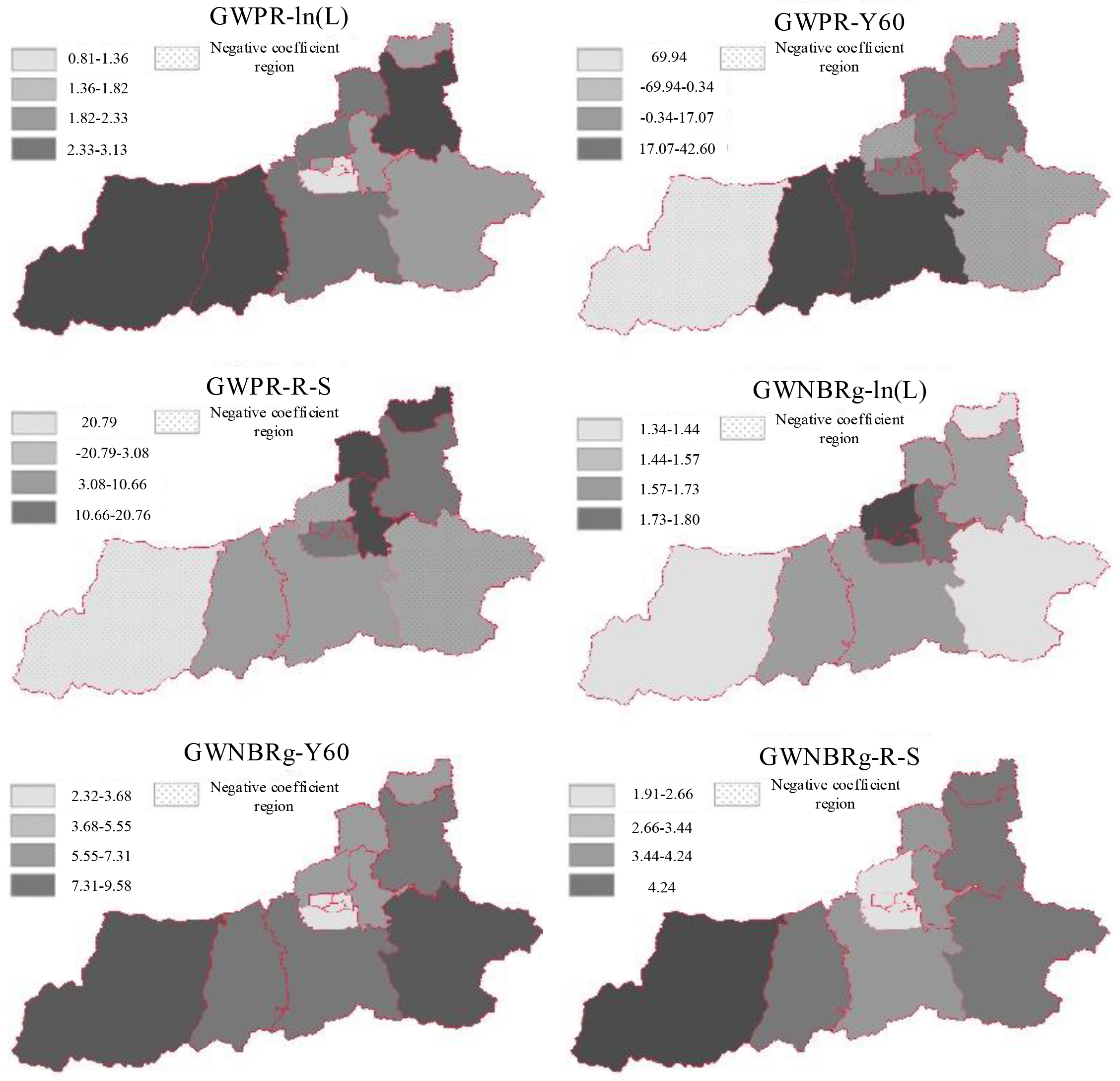

As can be seen from Fig. 2, the regression intercept and y of GWPR model and GWNBR model_60 and R-S variables are negative, and there are many low value areas and negative correlation areas in GWPR model, and the regression intercept and Y_ The maximum values of 60 and R-S variables do not exceed 4, 43 and 21. The coefficients of all variables in GWNBR model are positive, and the low value area accounts for a large proportion in the whole picture. There are some differences in the coefficients between GWPR model and GWNBR model, which may be caused by the multicollinearity between local coefficients. At the same time, it is found that there is little difference in the estimation range of the variance expansion coefficient of the two models. At the same time, the statistical significance of the model coefficient is calculated to obtain y in the GWPR model_ The variable coefficient of 60 ( $-$ 69.94 $\sim$ 42.60) is at the level of 10%, and the negative correlation area of 75% is not significant; R_ The variation range of s variation coefficient is similar, and the negative correlation coefficient of each region is not significant. In the GWNBR model, the coefficient value of the variable changes little, ranging from $-$ 3.64 to 28.43. The negative correlation area is not significant at the 10% level, R_ The above results show that the multicollinearity between local coefficients is not the cause of coefficient anomalies. At the same time, taking the global value of GWNBR of 0.23 as the overdispersion parameter, the spatial distribution of the coefficients and overdispersion parameters of the model are statistically plotted as shown in Fig. 3.

Figure 3.

Spatial distribution of GWNBR coefficients and over-dispersion parameters.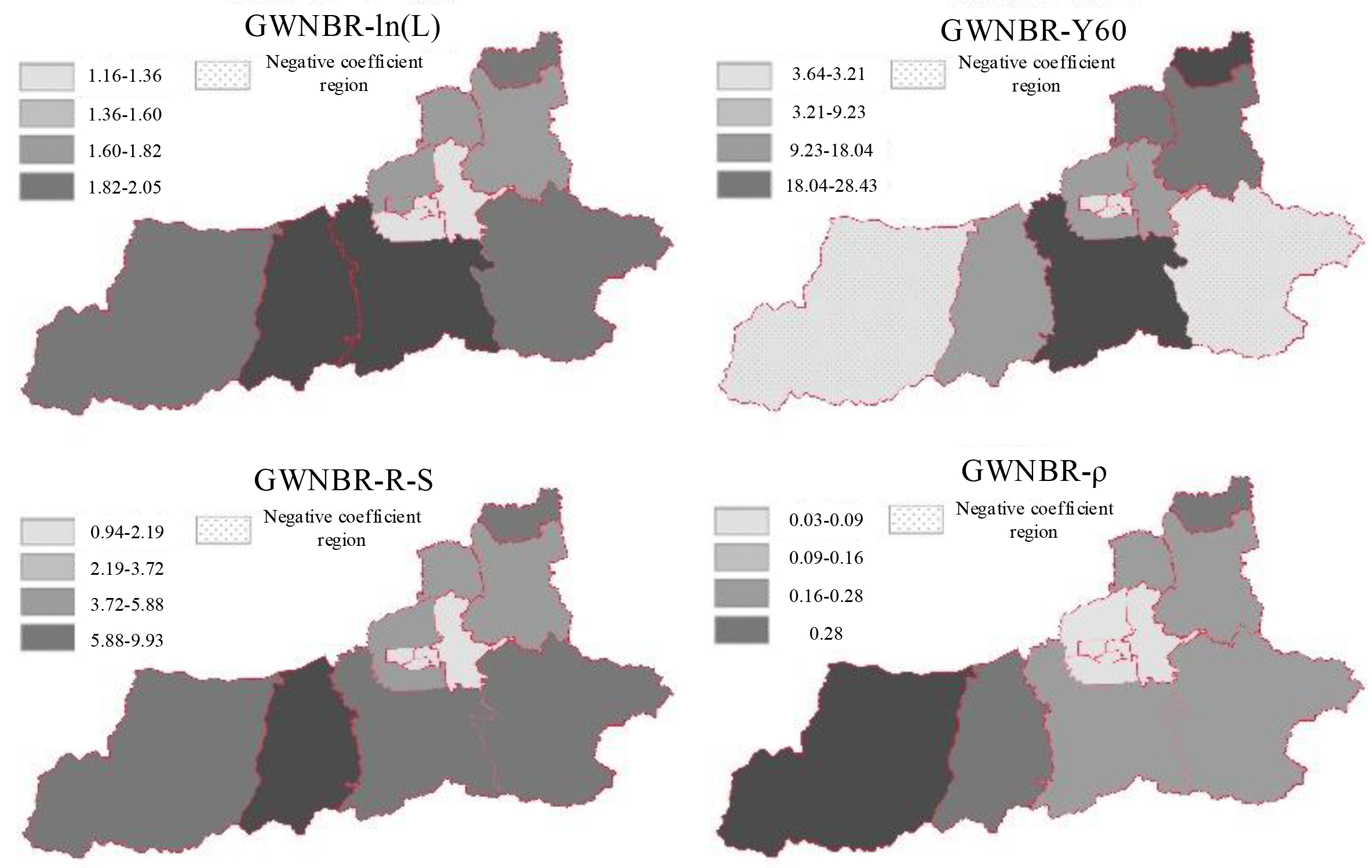

As can be seen from Fig. 3, the regression intercept and y of GWNBR model_ 60 and R-S variables are in the positive range, and the negative correlation area is less than that of GWPR model in Fig. 3. Compared with Fig. 3, the variables of the proportion of middle-aged and elderly people and the proportion of straight-line depot accidents in GWPR model in 13 regions show negative values in 4 regions and 3 regions respectively; In the GWNBR model, the variable changes to 2, and the area of 0 shows a negative value, indicating that the excessive dispersion of traffic accidents has a greater impact on the model coefficients. At the same time, it is found that the overdispersion parameter in GWNBR changes with space, and the spatial distribution is quite different. Its value shows a decreasing trend from southwest to northeast, that is, the value of overdispersion parameter is lower in the middle and Southeast, and increases in the West and north of the city. The value of the excessive dispersion coefficient is closely related to the interpretation ability between the models, and the change of high regional traffic volume will also increase the excessive dispersion parameter coefficient in the GWNBR model, which makes the model stronger in the interpretation of variable data.

3.4 Adjustment measures and spatial dependence

Use root mean square error (RMSE), AICc criterion and ML to quantify and analyze the performance of the comparison model. RMSE can be expressed as:

$\displaystyle\textit{RMSE}=\sqrt{\frac{1}{o}\sum{({y_{o}-y_{b}})^{2}}}$ (16)

In Eq. (16), $y_{o}$ is the observed value of the dependent variable, $y_{b}$ is the predicted value of the model, and $o$ is the sample size. In addition to the above indicators, the Moran index is used to determine the spatial dependence of the model. The null hypothesis used by Moran test is independent or spatial randomness has zero value. The Moran test varies between $-$ 1 and 1, where a value of 0 indicates a lack of correlation. The closer to 1, the higher the correlation between neighbors and the stronger the data concentration. The closer to $-$ 1, the more scattered the data and the lower the correlation between neighbors.

The formula in Da Silva and Fotheringham’s study is introduced [15], as shown in Eq. (17).

$\displaystyle\alpha=\varepsilon({p_{e}/p})$ (17)

where $p_{e}$ represents the effective number of discrete parameters. The goodness of fit indexes of global model and local model are as Table 3. So, for a GWNBR in Table 3 and for 5% significance level, the new alpha is 0.05/(33/8) $=$ 0.012.

Table 3

Adjustment of traffic accident model variables

Model	Bandwidth	Effective number of parameters	RMSE	2LL	AICc
NB	–	8.0	69.7	$-$ 1317	1378
GWPR	12	65.6	26.5	$-$ 1164	1710
GWNBRg	94	13.4	53.7	$-$ 1284	1352
GWNBR	34	33.0	40.6	$-$ 1178	–

According to Table 3, the NB global model has the worst adjustment effect on RMSE and ML, followed by GWNBRg, GWNBR and GWPR models. Because the local GWNBRg and GWNBR models are not easily affected by extreme values, the RMSE adjustment is worse than GWPR. The local GWNBRg and GWNBR model bandwidth size and the spatial variation of model coefficients are more uniform than the GWPR model. The best performance of AICc is the GWNBRg value of 1352, followed by NB. The performance of GWPR is poor due to excessive discrete data.

The comparison of the spatial autocorrelation values and P-values of the four models is as Table 4.

Table 4

Spatial correlation of model residuals

Model	Moran index	$P$ value
NB	0.20	0.00
GWPR	$-$ 0.11	0.01
GWNBRg	0.13	0.00
GWNBR	$-$ 0.01	0.49

According to Table 4, since the over-dispersion parameter used in the GWNBRg model uses a constant value $\rho=0.23$ , the spatial autocorrelation effect of the GWPR and GWNBRg local models in reducing residuals is not significant, but the effect is more significant than that of the NB model. The spatial autocorrelation of the residuals of the GWNBR model is significantly reduced, and the significance level is 5%, which reduces the spatial heterogeneity of the data. The unbiased estimation is compared with the NB, GWPR and GWNBRg models. The road length coefficient is related to the amount of traffic data to a certain extent. The longer the road length, the more vehicles it can accommodate, which virtually reduces the risk of road traffic accidents. Among them, roads in different directions will form a regional traffic road network. Therefore, according to the spatial presentation form of traffic data, the parameters are set in four directions of southeast, northwest and northwest, and the road length coefficients on different parameters are explored to better realize the analysis of traffic data. The statistical results of traffic data processing of different models are shown in Table 5.

Table 5

Statistical table of traffic data processing coefficients under different models

Model	GWPR model	GWNBRg model	GWNBR model
	Coefficient	Coefficient	Coefficient
North	0.264	0.261	0.689
South	0.743	0.279	0.274
West	0.526	0.276	0.238
East	0.211	0.258	0.527
Central section	$-$ 0.211	0.253	$-$ 0.162

The correlation coefficient of road length coefficient has a negative correlation with the risk of road traffic accidents in this area. It can be seen from Table 5 that the accident risk in the northern part of Xi’an is higher than that in the southern part of Xi’an in terms of the spatial distribution of road length coefficient (L) of GWNBR model. The reason is that the road network in the northern part is relatively dense and there is a large gap between the northern part and the development of the southern region. In the GWPR model, the correlation coefficient in the south of the city is relatively high, and the correlation coefficient in the central and eastern regions is negatively correlated. The spatial variation of GWNBRg model is more uniform, and the correlation coefficient in the central and eastern regions is small. When moving to the southeast and southwest, the correlation coefficient gradually increases. In the GWNBR model, the correlation coefficients of the central and southwest regions are the lowest.

4. Conclusion

In this paper, GWNBR model is used to analyze the accident risk in different areas of Xi’an. Using geographical weighted regression model and negative binomial regression model, this paper makes a comparative analysis of Xi’an expressway, and then establishes a traffic accident risk assessment model. The results show that GWNBR model effectively considers the influence of risk factors on geospatial elements in residual analysis, and the spatial autocorrelation of residual is significantly reduced, with a significance level of 5%. The negative correlation coefficient area of GWNBR model is lower than that of GWPR model, and the interference between traffic accident frequency and explanatory variables is less affected by spatial heterogeneity, indicating that GWNBR model has better effect in the risk analysis of over discrete road traffic accidents. When analyzing the actual data, the spatial coefficient of the model shows a decreasing trend from south to east, indicating that the continuous reduction of traffic accident risk is also consistent with the actual situation, and has good application value and early warning function, so as to reduce the occurrence of highway accidents.

References

Gao

Ren

. A deep learning approach for imbalanced crash data in predicting highway-rail grade crossings accidents. Reliab Eng Syst Saf. 2021; 216: 108019.

Yakimov

. Methods for assessing road traffic accident risks with changes in transport demand structure in cities. Transp Res Procedia. 2020; 50: 727-734.

Naumov

Otmakhova

Krasnykh

. Methodological approach to modeling and forecasting the impact of the spatial heterogeneity of the COVID-19 spread on the economic development of Russian regions. Comput Res Model. 2021; 13(3): 629-648.

Duan

Tang

Liu

. Study on the applicability of IHSDM in accident prediction of freeway of high proportion of bridges and tunnels in mountain area. Highway Eng. 2018; 43(3): 70-76.

Zhang

Kong

. Drivers’ route guidance model based on different risk propensity. China Saf Sci J. 2020; 30(5): 108-114.

Zhang

Huang

Sang

Sun

Chen

. Traffic accident prediction based on Markov chain cloud model. IOP Conf Ser: Earth Environ Sci. 2020; 526(1): 012188.

Middela

Ramadurai

. Incorporating spatial interactions in zero-inflated negative binomial models for freight trip generation. Transp. 2020; 48(4): 2335-2356.

Silva

Rodrigues

TCV

. Geographically weighted negative binomial regression-incorporating overdispersion. Statistics and Computing. 2014; 24: 769-783.

Yasin

Suryani

Kartikasari

. Graphical interface of geographically weighted negative binomial regression (GWNBR) model using R-Shiny. J Phys: Conf Ser. 2021; 1943(1): 012155.

10.

Luo

Yang

Yin

. Outliers-robust CFAR detector of gaussian clutter based on the truncated-maximum-likelihood-estimator in SAR imagery. IEEE Trans Intell Transp Syst. 2020; 21(5): 2039-2049.

11.

Roozbeh

Najarian

. Efficiency of the QR class estimator in semiparametric regression models to combat multicollinearity. J Stat Comput Simul. 2018; 88(7-9): 1804-1825.

12.

Xue

. Hierarchical geographically weighted regression model. J Quantum Comput. 2019; 1(1): 9-20.

13.

Qin

Huang

Zhang

, et al. Carbon dioxide emission driving factors analysis and policy implications of Chinese cities: Combining geographically weighted regression with two-step cluster. Sci Total Environ. 2019; 684: 413-424.

14.

Harris

. A simulation study on specifying a regression model for spatial data: Choosing between autocorrelation and heterogeneity effects. Geogr Anal. 2019; 51(2): 151-181.

15.

Da Silva

Fotheringham

. The multiple testing issue in geographically weighted regression. Geographical Analysis. 2016; 48(3): 233-247.

Application analysis of highway traffic accident risk model based on geographically weighted negative binomial regression

Abstract

Keywords

1. Introduction

2. Road traffic accident risk analysis method based on GWNBR model

2.1 Negative binomial distribution model

3.1 Study area selection and data source

Table 1 Statistical variables of highway traffic accidents

3.3 Geographically weighted regression model coefficient estimation

References

Table 1
Statistical variables of highway traffic accidents