Real-time anomaly attack detection based on an improved variable length model

Abstract

This paper uses a real-time anomaly attack detection based on improved variable length sequences and data mining. The method is mainly used for host-based intrusion detection systems on Linux or Unix platforms which use shell commands. The algorithm first generates a stream of command sequences with different lengths and subsumes them into a generic sequence library, de-duplicats and sortes shell command sequences. The shell command sequences are then stratified according to their weighted frequency of occurrence to define the state. Next, the behavioural patterns of normal users are mined to output the state stream and a Markov chain is constructed. Then, the state sequences are calculated based on a primary probability distribution and a transfer probability matrix. The System will check decision values of the short sequence stream. Finally, the decision values of the behavioural sequences are analysed to determine whether the current session user is behaving abnormally. The improved algorithm introduces the concept of multi-order frequencies and proposes a new separation mechanism. The extension module is integrated into the variable length model. By comparing the performance of the old and new separation mechanisms on the SEA dataset and the self-made dataset (SD), it is found that the improved model greatly improves the performance of the model and shortens the running time.

Keywords

Variable length model Markov new separation mechanism weighted frequency

1. Introduction

Most current intrusion detection systems use anomaly detection techniques, which have the advantage of detecting unknown types of attacks and do not require much a prior knowledge. So anomaly detection has been widely studied as an important branch of network intrusion detection.

In practical anomaly attack detection, the training data for detection is often insufficient due to the variability of user behaviour, which requires that the detection model should have fault tolerance, generalisation ability and adaptability. In recent years, research has been conducted at home and abroad on the application of data mining, statistical theory, machine learning, deep learning and other techniques in anomaly attack detection. However the common problems of these anomaly attack detection methods are lack of adaptability to changes in user behaviour, stability and fault tolerance of detection performance, and need improve detection accuracy.

To overcome the above weaknesses, this paper uses a real-time anomaly attack detection method based on improved variable length sequences and data mining. The algorithm first generates a stream of command sequences and subsumes them into a generic sequence library, de-duplicats and sortes shell command sequences. The shell command sequences are then stratified according to their weighted frequency of occurrence to define the state. Next, the behavioural patterns of normal users are mined to output the state stream and a Markov chain is constructed. Then, the probabilities of short state are calculated based on the primary probability distribution A and the transfer probability matrix P. The System will check decision values of the short sequence stream. Finally, the decision values of the behavioural sequences are analysed to determine whether the current session user is behaving abnormally.

The improved algorithm introduces the concept of multi-order frequencies and proposes a new separation set mechanism. The extension module is integrated into the variable length model. By comparing the performance of the old and new separation mechanisms on the SEA dataset and the self-made dataset (SD), it is found that the improved model greatly improves the performance of the model and shortens the running time. The host real-time monitoring script is conjuncted in the detecting host, we achieve the real-time anomaly attack detection.

2. Current status of research

Machine learning approaches are mostly used for anomaly attack detection. Lane [3] investigated anomaly attack detection based on HMM. They used HMM to build a fame of the normal behaviour of legitimate users at user interface layer and trained the HMM using the Baum-Welch algorithm. The main advantage of this approach is the high detection accuracy and its disadvantage is poor detection efficiency. Kholidy [9] proposed DDSGA. To improve the performance, Qiu [10] combined the HMM with the the SA module. Xinguang Tian [12] mines user behaviour patterns by using variable length shell command sequences to and employs a similarity metric. Xi Xiao [13] greatly reduced the number of states, thereby reduced memory consumption. The model uses the weighted frequency of a variable-length sequence. He achieved the best results compared to previous models based on Markov chains.

Figure 1.

Flowchart of anomaly attack detection algorithm in the variable length model.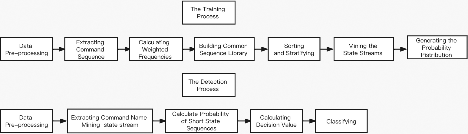

3. Anomaly detection system design

The system uses the SEA dataset to evaluate the improved variable-length Markov chain algorithm and the model trained on the RD dataset identifies host anomalous behaviour. The RD dataset is derived from the system shell command log and the shell commands entered by the user in real time. The training process of the variable-length model in the anomaly detection algorithm is: pre-processing the training data of the RD dataset, extracting only the command names, extracting command sequence streams of different lengths according to the parameters, calculating the weighted frequencies of the sequence streams and building a common sequence library, sorting in descending order according to the weighted occurrence frequency and stratifying, and finally mining the state streams of the training data through data mining, and finally generating the probability distribution. The detection process is: pre-processing the data, extracting only the command names, data mining and getting the state stream according to the initial state distribution A generated in the training phase and the state transfer probability matrix P, setting a sliding window to calculate the probability of short state sequences, and finally calculating the decision value and classifying it according to a pre-set threshold.

This paper proposes a new separation mechanism. The flowchart is shown in Fig. 2.

Figure 2.

Flowchart of the new separate pooling mechanism.

4. Implementation of anomaly detection system

4.1 Training module implementation in the variable length model

1) Data pre-processing

For the raw training data (OS) without any processing, only the command names are retained, filtering command parameters and events. Then we get finally training data (S). We let $r$ denote the length of the data and COM denote the name of the shell command ( $s_{j}\in\text{COM}$ ). Then the training data is $S=(s_{1},s_{2},\ldots,s_{r})$ .

2) Extraction of variable length sequences

[14] gives the definition formula of variable L and $\overline{S_{q}^{k}}$ ,which is Formula 3a in [14], So we don’t describe them again. The sequence stream $\overline{\overline{S^{1}}},\overline{\overline{S^{2}}},\ldots,\overline{% \overline{S^{W}}}$ is generated, where the sequence stream $\overline{\overline{S^{k}}}(1\leqslant k\leqslant W)$ is defined as:

$\displaystyle\overline{\overline{S^{k}}}=(\overline{S_{1}^{k}},\overline{S_{2}% ^{k}},\ldots,\overline{S_{r-l(k)+1}^{k}})$ (1)

Thus, in the extraction of variable-length sequences stage, a variable-length sequence library $T$ with length $W$ can be generated based on the given training data $S$ , the set of lengths L.

$\displaystyle T=\{\overline{\overline{S^{1}}},\overline{\overline{S^{2}}},% \ldots,\overline{\overline{S^{W}}}\}$ (2)

Assume that the training data S is (‘cpp’, ‘sh’, ‘xrdb’, ‘mkpts’, ‘env’, ‘ksh’, ‘userenv’, ‘wait4wm’, ‘ksh’, ‘userenv’, ‘wait4wm’). Assuming L $=$ {2, 3}. An example diagram of a variable-length sequence set $T$ is shown in Fig. 3.

Figure 3.

A variable length sequence set T.

3) Calculation of weighted frequencies

[14] calculates the weighted frequency of occurrence of different sequences, the number of occurrences of the sequence $\overline{S_{q}^{k}}$ , the frequency of occurrence of $\overline{S_{q}^{k}}$ in $\overline{\overline{S^{k}}}$ . So the first-order weighted frequency of occurrence is defined:

$\displaystyle(wf_{q}^{k})_{1}=e_{1}(k)\cdot f(\overline{S_{q}^{k}})$ (3)

We introduce multiple orders and the real implementation of the algorithm is the “second-order” algorithm.

$V$ denotes the order and the v order weighted frequency is defined as follows:

$\displaystyle({wf}_{q}^{k})_{0}\equiv\overline{S_{q}^{k}}$ (4) $\displaystyle({wf}_{q}^{k})_{v}=e_{v}(k)\cdot f((wf_{q}^{k})_{v-1})$

$f(({wf}_{q}^{k})_{v})$ is defined as follows:

$\displaystyle f(({wf}_{q}^{k})_{v})=\frac{(n_{q}^{k})_{v}}{r-l(k)+1}$ (5)

Where $(n_{q}^{k})_{v}$ represents the number of times of $(w_{q}^{k})_{v}$ appeared in the sequence stream $\overline{\overline{(S^{k})_{v}}}$ . Assuming $v=$ 1, $(n_{q}^{k})_{v}$ represents the number of times appeared in the sequence stream $\overline{\overline{S^{k}}}$ , which corresponds to the first-order weighted frequency: $(wf_{q}^{k})_{1}=e_{1}(k)\cdot f(\overline{S_{q}^{k}})$ . The v-order weighted frequency actually extracts features from the v-1 weighted frequency again, and theoretically the larger the $v$ is, the more features are extracted and the better the model performs are. Therefore, this paper implements the model based on $v=$ 2.

So if $v=$ 2, First-order weighted frequencies and second-order weighted frequencies are obtained. Assume L $=$ {2, 3}, E1 $=$ {2, 3} and E2 $=$ {2, 3}.

In the case of $k=$ 1 (l(1) $=$ 2), the examples are shown.

Table 1

Example $k=$ 1

Serial number $q$	Orders $s_{q}$	Serials $(w_{q}^{k})_{0}$	Number of first-order occurrences $(n_{q}^{k})_{0}$	First order weighted frequencies $(wf_{q}^{k})_{0}$	Number of second order occurrences $(n_{q}^{k})_{1}$	Second order weighted frequency $(wf_{q}^{k})_{0}$
1	cpp	(cpp, sh)	1	1/5	6	6/5
2	sh	(sh, xrdb)	1	1/5	6	6/5
3	xrdb	(xrdb, mkpts)	1	1/5	6	6/5
4	mkpts	(mkpts, env)	1	1/5	6	6/5
5	env	(env, ksh)	1	1/5	6	6/5
6	ksh	(ksh, userenv)	2	2/5	4	4/5
7	userenv	(userenv, wait4wm)	2	2/5	4	4/5
8	wait4wm	(wait4wm, ksh)	1	1/5	6	6/5
9	ksh	(ksh, userenv)	2	2/5	4	4/5
10	userenv	(userenv, wait4wm)	2	2/5	4	4/5
11	wait4wm	N	N	N	N	N

In the case of $k=$ 2 (i.e. l(2) $=$ 3), the examples are shown in Table 2.

Table 2

Example table for $k=$ 2

Serial number $q$	Orders $s_{q}$	Serials $(w_{q}^{k})_{0}$	Number of first-order occurrences $(n_{q}^{k})_{0}$	First order weighted frequencies $(wf_{q}^{k})_{0}$	Number of second order occurrences $(n_{q}^{k})_{1}$	Second order weighted frequency $(wf_{q}^{k})_{0}$
1	cpp	(cpp, sh, xrdb)	1	1/3	7	7/3
2	sh	(sh, xrdb, mkpts)	1	1/3	7	7/3
3	xrdb	(xrdb, mkpts, env)	1	1/3	7	7/3
4	mkpts	(mkpts, env, ksh)	1	1/3	7	7/3
5	env	(env, ksh, userenv)	1	1/3	7	7/3
6	ksh	(ksh, userenv, wait4wm)	2	2/3	2	2/3
7	userenv	(userenv, wait4wm, ksh)	1	1/3	7	7/3
8	wait4wm	(wait4wm, ksh, userenv)	1	1/3	7	7/3
9	ksh	(ksh, userenv, wait4wm)	2	2/3	2	2/3
10	userenv	N	N	N	N	N
11	wait4wm	N	N	N	N	N

4) Building a generic sequence library

Repeated sequences $(w_{q}^{k})_{0}$ are appeared in Tables 1 and 2, such as (ksh, userenv). The commands entered by users tend to possess a certain pattern, so in the case of actual training data with thousands of shell command, there is a high probability that duplicate sequences will occur. Repeated sequences also have the same weighting frequency, which increases the memory and computational cost in practice. Therefore it is necessary to extract all the different short sequences from $\overline{\overline{S_{k}}}(\overline{t_{1}^{k}},\overline{t_{2}^{k}},\ldots,% \overline{t_{m(i)}^{k}})$ , so the purpose of de-weighting is achieved.

All different sequences are grouped together in a common sequence library (LGS).

$\displaystyle LGS=(\overline{t_{1}^{1}},\overline{t_{2}^{1}},\ldots,\overline{% t_{m(1)}^{1}},\overline{t_{1}^{2}},\overline{t_{2}^{2}},\ldots,\overline{t_{m(% 2)}^{2}},\ldots\overline{t_{1}^{W}},\overline{t_{2}^{W}},\ldots\overline{t_{m(% W)}^{W}})$ (6)

According to the v-order weighted frequencies mentioned above, the v of generic sequence library will be generated.

Assuming L $=$ {2, 3}, E1 $=$ {2, 3}, E2 $=$ {2, 3}. An example diagram of the generic sequence library LGS1 is shown in Fig. 4 and an example diagram of the generic sequence library LGS2 is shown in Fig. 5.

Figure 4.

LGS1 example.

Figure 5.

LGS2 example.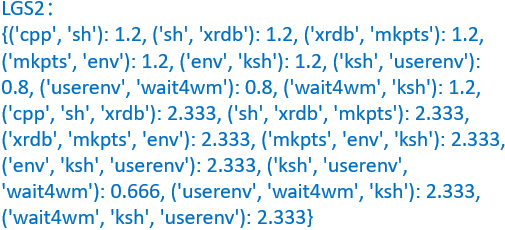

5) Sort and merge in layers

Markov chains are actually models that portray transfer between states over time. Common Markov chain applications such as predicting the weather correspond to many states, e.g. sunny, rainy, snowy, etc. However, for shell sequences there is no state, so it is necessary to define states for shell sequences. If a shell sequence is used directly as a state, such as the sequence (cd, ls) corresponding to a state, then for thousands of training data, thousands of states will be defined. This will definitely leads to overfitting of the model and high computational overhead. So it is not suitable for real-time detection. Therefore, in order to define states, the features of the shell sequences need to be found in some way, and the sequences are grouped together and defined as one state based on the same features.

The method of extracting features in this paper uses the weighted frequency, which defines the state according to the magnitude of the frequency. The larger frequency of the sequence defines the state as 1, and the smaller sequence frequency defines the smaller state value. Therefore, it is necessary to sort each generic sequence library in descending order, and the generic sequence library is defined as G after sorting in descending order.

The descending sorted generic sequence library G is divided into N sets, denoted as $\Lambda^{v}=\{\Lambda_{0}^{v},\ldots,\Lambda_{N-1}^{v}\}$ . Clearly, for the same training data v descending sorted generic sequence libraries G are generated, with different G denoted as Gv. It is worth noting that for different Gv, each sequence has a different weighting frequency and the sequence order is different, but the length of Gv and the corresponding sequence elements are the same.

Giving N $=$ 3, Figs 6 and 7 show examples of G1 and G2, respectively, after separation.

Figure 6.

Example diagram of separation G1.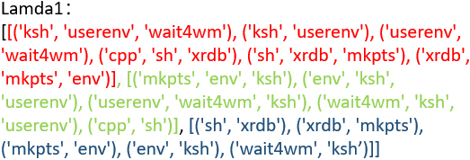

Figure 7.

Example diagram of separation G2.

6) Mining user behaviour to define states

After separating the set and defining the state, the next step is to mine the training data for patterns that reflect the user’s behaviour, which is divided into two main parts: defining the state and mining the user’s behaviour. The core idea of mining the user behaviour pattern function is to mine the training data behaviour through the generated Lamda1 and Lamda2. Assuming L $=$ {2, 3}, Fig. 8 represents the mining user behaviour process for the example training data.

Figure 8.

Example diagram for mining user behaviour.

The define state function passes an index to the function of mining user behaviour. The index points to the first shell command. Assuming L $=$ {2, 3}, the blue part is the initialised sequence of length 2 and the green part is the sequence of length 3. At this point, comparing the weighted frequency corresponding to (cpp, sh) with the weighted frequency corresponding to (cpp, sh, xddb). The comparison reveals that the weighted frequency corresponding to (cpp, sh, xrdb) is greater, so the function of mining user behaviour returns the sequence (cpp, sh, xrdb). This paper uses a weighted frequency processing the sequence of $v=$ 2 to obtain Lamda1 as well as Lamda2, so the function of mining user behaviour obtains two behaviour sequences, respectively, according to Lamda1 and Lamda2. So the function finally returns [first-order behaviour sequence, second-order behaviour sequence].

After (cpp, sh, xrdb) is mined, the index will increase the length of the mined sequence, which points to mkpts. Since Lamda is formed from training data, it must be able to mine the behavioural sequence for training data. But for unknown detection data, it is likely that the sequence has never been in Lamda. When the comparison finds that the weighted frequency frequency corresponding to (cpp, sh) and the weighted frequency corresponding to (cpp, sh, xddb) are both 0, null is returned and the index is added by 1.

After a number of mining behaviours, the index points to userenv, at which point the sequence marked in red is found to be of length 2. Noting that 2 $<$ l(W) $=$ 3, it is not possible to compare with the case of length 3, so the sequence is discarded. The mining of user behaviour ends.

Next we will describe the definition of the state function. This function calls the behaviour sequence obtained from the function of mining user behaviour: [first-order behaviour sequence, second-order behaviour sequence]. Then we define a state for the behaviour sequence based on the Lamda after separating the sets. For the same sequence, the second-order method returns two sequences of behaviours. Then the indexes of the first-order behaviour sequence in Lamda1 and the second-order behaviour sequence in Lamda2 are found and assigned to state1 and state2 respectively. In data mining, a sequence can only be defined as one state, hence we do the normalisation process.

For the case $v=$ 2, we define $\textit{state}=\textit{state}1\cdot N+\textit{state}2$ ; for the case $v=n$ , we define $\textit{state}=\textit{state}_{1}\cdot N^{V-1}+\textit{state}_{2}\cdot N^{V-2}% +\ldots+\textit{state}_{n}$ .

The algorithm defines the state of the Markov chain through a variable-length sequence of shell commands. This enhances the model’s ability to mine normal behavioural features and its adaptability to variable user behaviour. In addition, the frequency-first based approach finds behavioural patterns in the set in Lamda’s order. This speeds up the matching time of the sequences.

By mining the user behaviour to define the states, the training data is processed to eventually form the state stream STATES, which lays the foundation for A and P.

7) Establishing probability distributions

The Markov chain consists of A and P. The state flow is obtained by defining the states and A and P are found based on statistical ideas.

For the second order method in the case $v=$ 2 state $=$ state1*N $+$ state2. IF N $=$ 3, then state € [0, 9]. Extending to the general solution, assuming $v=$ 3, for a given set number N, the final state transfer probability matrix P of (N ${}^{2}$ $+$ 1)*(N ${}^{2}$ $+$ 1) is generated.

4.2 New module for separating sets (improved algorithm)

The core of the idea in the old mechanism for separating sets is to equate as much as possible the generic library of sequences sorted in descending order G. Assuming N $=$ 3, for training data of length 6, it is divided into three lists of length 2. So G is a set of shell sequences sorted in descending order according to weighted frequencies. The final set of separated states is obtained based on a descending order. Such a separation mechanism based on the idea of equating is not sensitive to the break in weighted frequencies and does not fully exploit the weighted frequency features corresponding to the sequences.

In order to furtherly mine the weighted frequency feature, This paper proposes a new separation set mechanism. For a sorted generic sequence library G of length K, the weighted frequencies of adjacent sequences are computed sequentially to obtain the set of differences $D=(d_{1},d_{2},\ldots,d_{k-1})(dr\geqslant 0,1\leqslant r\leqslant K-1)$ . If the number of separated sets is N, extract the largest N-1 differences in the D-value set D to obtain the set of maximum weighted frequency differences. Based on the set of maximum weighted frequency differences I, find the corresponding set of sequence indices.

Finally, the final Lamda is obtained by dividing the set of N sets according to the set of sequences Index. If a sequence of length 5 is {(cpp, sh), (spp, sh, xrdb), (ksh, userenv), (cpp), (vim, sqlmap)}, and the sequence corresponds to a weighted frequency of (2, 1.5, 1.4, 1.3, 0.9).

Figure 9.

Example of comparison of separation mechanisms.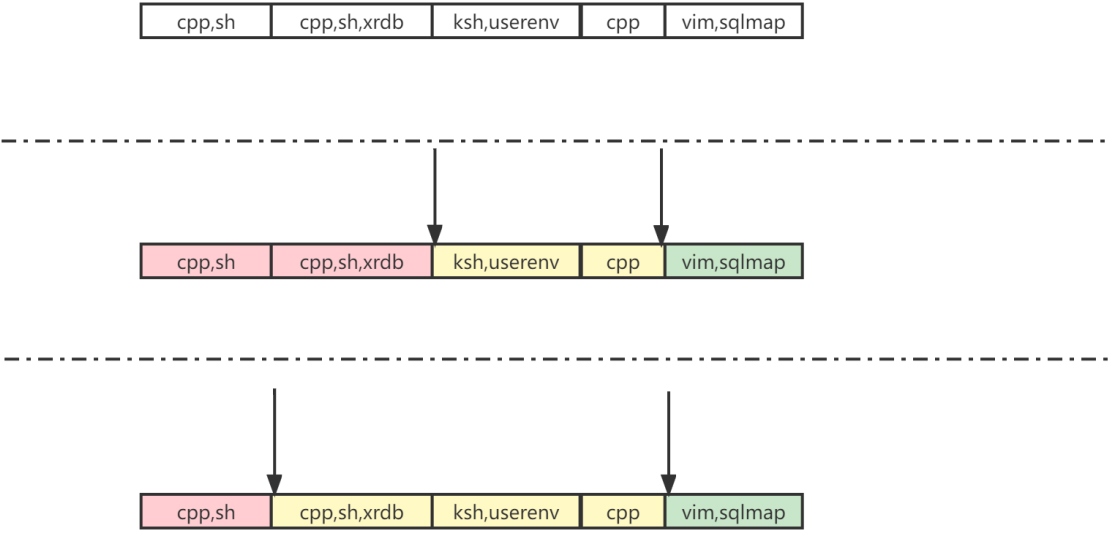

The sequence weighted frequencies are (2, 1.5, 1.4, 1.3, 0.9). The old separation mechanism does not consider the specific real-value distribution of the weighted frequencies, and divides the set into two sets of length 2 and one set of length 1 based on the idea of equal division. The new separation mechanism, on the other hand, calculates the D-value set D $=$ (0.5, 0.1, 0.1, 0.4) for the real-valued distribution, so the set of maximum weighted frequency differencesis I $=$ (0.5, 0.4), and the corresponding set of sequence indicesis Index $=$ {0, 3}. So the new separation mechanism will divide the set into the first one of length 1, the middle one of length 3, and the last one of length 1. The separated sets are marked in pink, yellow and green respectively.

4.3 Variable length model detection module

1) Calculating the probability of a short state sequence

After Data pre-processing and Mining data behaviour to define states like the training data. In a real-time host-based intrusion detection scenario, the task is to find the probability of a sequence of states occurring simultaneously to obtain the final decision value, rather than to know the current state and predict the next state. Therefore the probability of the states occurring simultaneously needs to be required,which is the joint distribution.

Defining u as the length of the short state sequence, the short state sequence is defined as $\overline{\sigma_{m}}=\{{\sigma_{m},\sigma_{m+1},\ldots,\sigma_{m+u-1}}\}$ . We can calculate the probability of the sequence according to Eq. (9).

$\displaystyle\Pr(\overline{\sigma_{m}})=a_{\sigma_{m}}\cdot p_{\sigma_{m+1}% \cdot\sigma_{m+2}}\ldots p_{\sigma_{m+u-2}\cdot\sigma_{m+u-1}}$ (7)

$u$ represents the simultaneous consideration of the states of $u$ moments to find the joint distribution.

4.4 Calculation of decision values

The decision value $D(n)$ can be calculated from the short state sequence probabilities obtained above with the sliding window, which is defined as follows:

$\displaystyle D(n)=\frac{1}{w}\sum_{m=n-w+1}^{n}(P(\delta_{m},\delta_{m+1})-% \eta),w\leqslant n\leqslant M-2+1$ (8)

Supposing that the state sequence obtained after the short state sequence processing is [03, 30]. If $w=2,\eta=0.1,P(0,3)=1/3$ and $P(3,0)=1/3$ the calculated decision value is:

$\displaystyle D(1)=\left[{\left({\frac{1}{3}-0.1}\right)+\left({\frac{1}{3}-0.% 1}\right)}\right]\cdot\frac{1}{2}\approx 0.2333$

4.5 Classification

The decision value is calculated and the given decision threshold $\lambda$ is used to determine whether the behaviour is abnormal or not. Assuming that $\eta$ is set to 0.3, the decision value calculated above is $D(1)\approx 0.2333<0.3$ and therefore the behaviour is judged to be abnormal.

5. Comparison of experimental results

The SEA dataset was used to demonstrate the improvement of the model with the new separation mechanism, while the SD dataset was used for practical testing.

5.1 Assessment methods

This experiment evaluates model performance with multiple metrics, using ROC curves for the SEA dataset and the area AUC of the ROC. In the experiment, the AUC average performance is evaluated for multiple users.

For $n$ users, the average AUC is defined as follows.

$\displaystyle\textit{AUCmeanm}=\sum\limits_{u}\frac{\mathop{\textit{AUC}}_{u}^% {m}}{n}$ (9)

In the SD dataset, the model was evaluated using the PR curve as well as the area AP of the PR curve.

5.2 Comparison and discussion of various algorithms

In order to demonstrate the advantages of the new separation mechanism, six algorithms were compared in this experiment: equal-length Markov chains (Markov), first-order Markov chains (MarkovF1), second-order Markov chains (MarkovF2), equal-length Markov chains with the new separation mechanism (Markov-N), first-order Markov chains with the new separation mechanism (MarkovF1-N1), second-order Markov chains with a new separation mechanism (MarkovF2-N2).

In order to fully evaluate the new separation mechanism, data statistics, two experimental evaluations and one additional experiment were carried out on the SEA dataset. At the same time, an algorithm comparison was also performed for the SD dataset, which is described in turn below.

5.3 SEA dataset

1) SEA dataset statistics

Although the SEA dataset collected the behaviour of 50 users and were randomly inserted by blocks of anomalous data, not all users had anomalous data. Figure 10 shows the anomalous data blocks for all users.

Figure 10.

Statistical chart of abnormal user data blocks.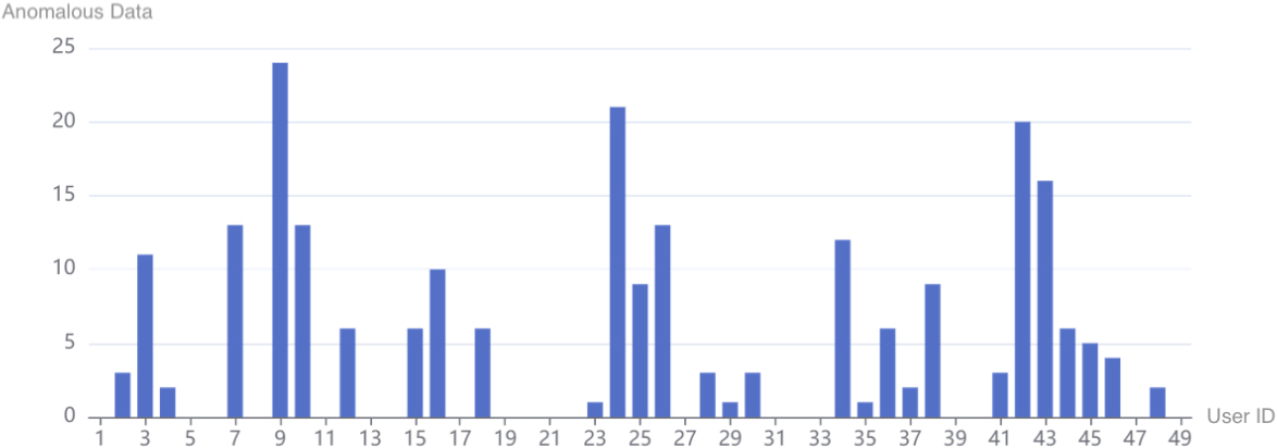

Table 3

Parameter space for the isometric method (Markov)

	Length set L	Separate set number N	Sliding window w	Probability threshold $\eta$
Scope	[1], [2], [3], [4], [5], [6], [7]	[2, 7]	[21, 81]	[0.05, 0.20]
Step length	None	1	5	0.01

Table 4

First-order method (MarkovF1) parameter space

	Length set L	Set of first order weights E1	Separate set number N	Sliding window w	Probability threshold $\eta$
Scope	[1, 2, 3], [2, 3, 4], [3, 4, 5],	[1, 2, 3], [1, 3, 5], [2, 3, 4],	[2, 7]	[21, 81]	[0.05, 0.20]
	[1, 3, 5], [2, 4, 6], [2, 5, 7]	[2, 4, 6], [3, 4, 5], [3, 5, 7]
Step length	None	None	1	5	0.01

Table 5

Second order method (MarkovF2) parameter space

	Length set L	Set of first order weights E1	Set of second order weights E2	Separate set number N	Sliding window w	Probability threshold $\eta$
Scope	Same as first-order	Same as first order	[1, 2, 3], [1, 3, 5], [2, 3, 4],	[2, 7]	[21, 81]	[0.05, 0.20]
	method L	method E1	[2, 4, 6], [3, 4, 5], [3, 5, 7]
Step length	None	None	None	1	5	0.01

Figure 11.

Comparison of the three algorithms for AUC.

Figure 12.

Comparison of old and new separation mechanisms.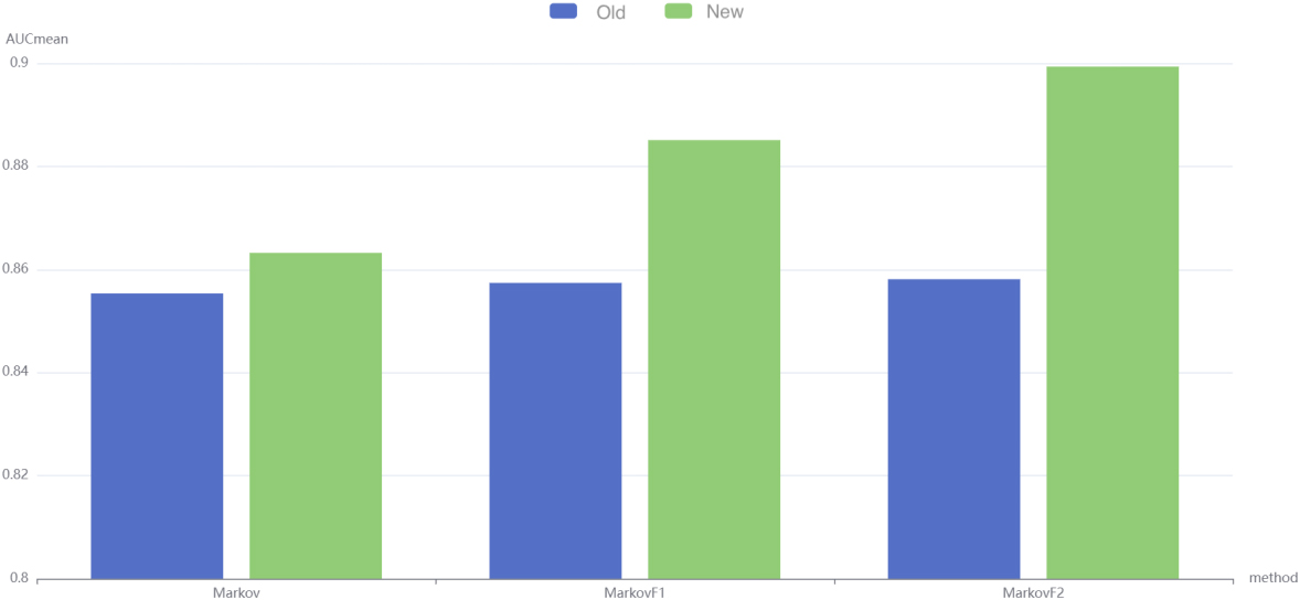

Figure 13.

MarkovF2-N2 performance as a function of w, N.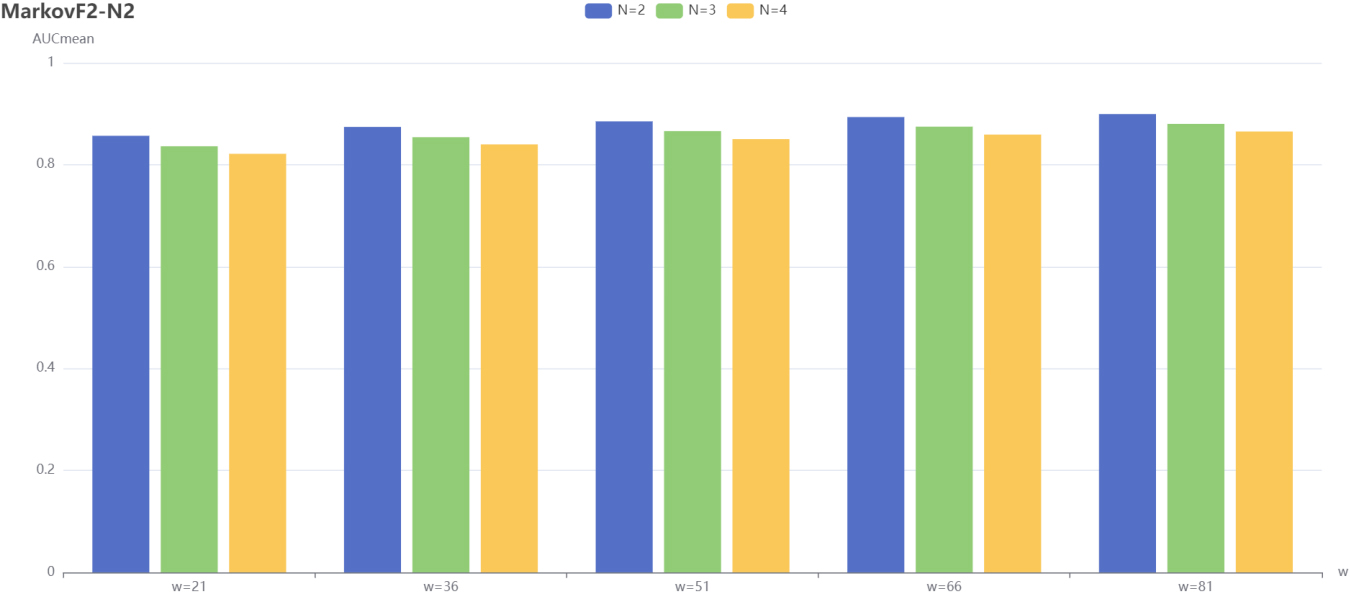

Figure 14.

MarkovF1-N1 performance versus w and N.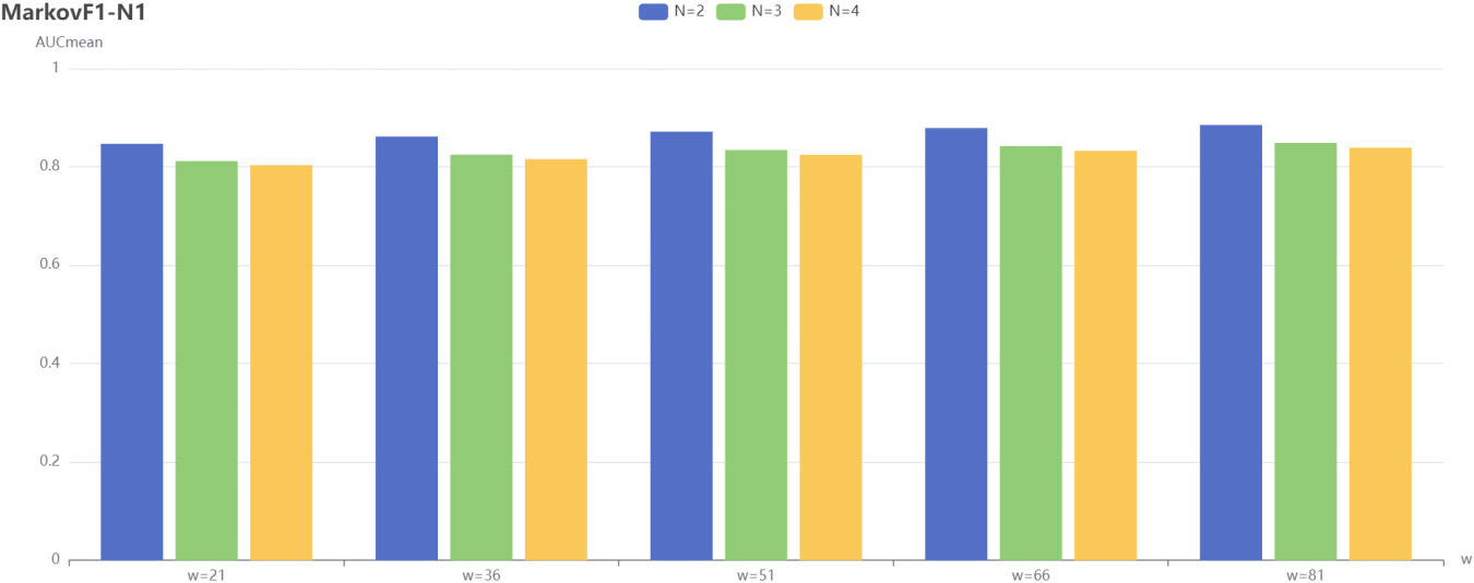

Figure 15.

Markov-N performance as a function of w, N.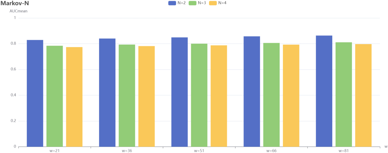

It can be seen that only 29 users dataset were inserted by random blocks of abnormal data and some users had only 1 or 2 blocks of abnormal data. Considering that the sliding window has a requirement for the number of users’ abnormal data, the top 20 users’ blocks of abnormal data are userd in the fellowing experiments.

2) Experiment 1: Top 20 user evaluation

Experiment 1 beganed with a model comparison of Markov, MarkovF1 and MarkovF2. Due to time constraints, this experiment was conducted by greedy search to find the optimal parameters in a given parameter range for the ROC curve area AUC comparison. For each algorithm, the sum of the AUCs of 20 users was obtained for each round of training, and then divided by 20 to obtain AUC ${}_{\text{mean}}$ , and the largest AUC ${}_{\text{mean}}$ was finally selected as the experimental result for this algorithm.

The ratio of training set: test set is 5000*20: 10000*20.

After a local search for the best parameters with the greedy algorithm, it was found that the second order method was slightly higher than the first order method and the first order was slightly higher than the equal length method. Figure 11 shows the comparison results.

Then, the new separation mechanism was introduced in the experiment, corresponding to the three algorithms Markov-N, MarkovF1-N1 and MarkovF2-N2, which were compared with the three algorithms Markov, MarkovF1 and MarkovF2 of the original separation mechanism, respectively. Figure 12 shows experimental results.

The experimental results show that the variable-length model based on second-order weighted frequencies outperforms the first-order variable-length model and the equal-length model. All of the models with the new separation mechanism achieve very significant improvement in AUC. The second-order method achieves the most significant improvement.

3) Additional experiments: Sliding window and number of separating sets

From Experiment 1, we can learn that for TOP20 users, the models that adopt the new separation mechanism are all improved from the original ones. Next, for the Markov-N, MarkovF1-N1 and MarkovF2-N2 algorithms, the effects of the sliding window w and the number of separation sets N on the models are explored.

Table 6

Comparison table between the old and new separation mechanisms

Algorithms	Old separation mechanism AUC/%	New separation mechanism AUC/%	Old separation mechanism Average running time/s	New separation mechanism Average running time/s
Markov	73.3415826549171	77.86977882836715	0.0124729	0.0119583
MarkovF1	81.07339022952598	90.65938064906572	0.0496336	0.0478224
MarkovF2	89.85833043145054	91.73547595673762	0.0726235	0.0692983

Figure 16.

Comparison of the effects of the old and new separation mechanisms for ROC curve area.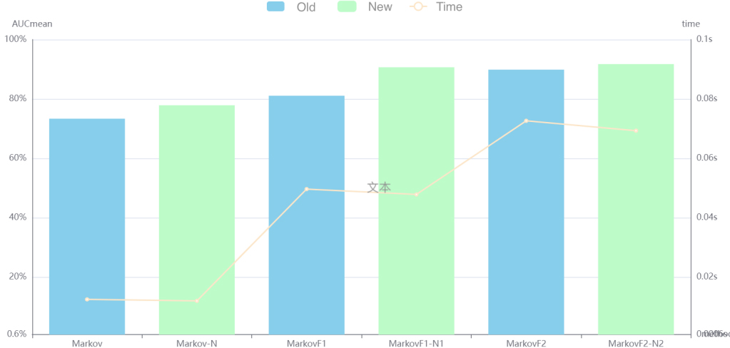

Figure 17.

Comparison of the effects of the old and new separation mechanisms for PR curve area.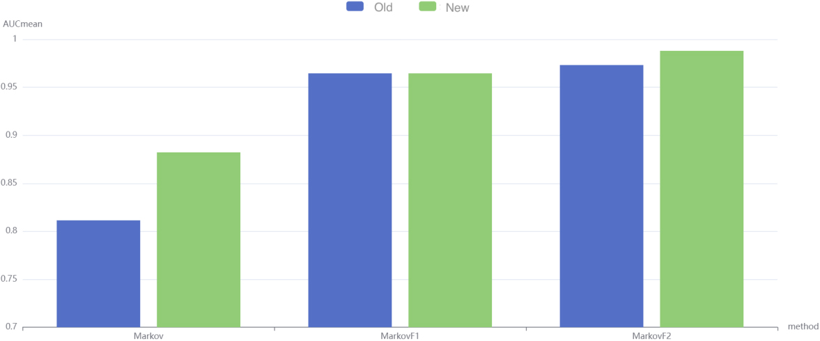

Figure 18.

PR graphs for the four algorithms.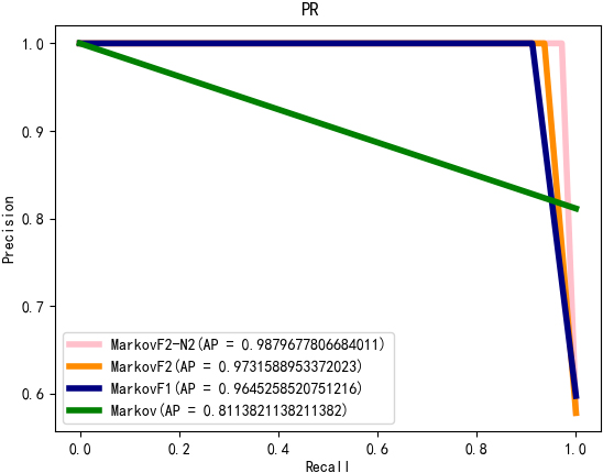

For all other hyperparameters the best parameters of the corresponding model are used. The sliding window w is set in the range [21, 36, 51, 66, 81] and the number of separation sets N is set in the range [2, 3, 4].

Figures 13–15 correspond to the relationships of the MarkovF2-N2, Markov-N and MarkovF1-N1 algorithms respectively.

The performance of all three algorithms, MarkovF2-N2, Markov-N and MarkovF1-N1, is shown. which increases with the sliding window w and decreases with the number of separation sets N.

4) Experiment 2: Four User (NU4) Assessment

Six models MarkovF2-N2, MarkovF1-N1, Markov-N, MarkovF2, MarkovF1, and Markov were compared for ROC area (AUC) by finding the optimal parameters within a given parameter range by grid search. The training detection times of the old and the new separation mechanisms were compared. Each algorithm runs one hundred times. The final training detection time is the running time of each algorithm divided by 100. So Training set: test set $=$ 5000*4: 10000*4.

Due to time constraints, the number of sets N was set uniformly to 2, the sliding window w to 21 and eta to 0.1.

The experimental results are shown in Fig. 16, where the dashes indicate the running time of the corresponding algorithms and the bars indicate the AUC of the corresponding algorithms. Table 6 indicates the specific parameters.

5.4 SD data set

For the SD dataset, six models MarkovF2-N2, MarkovF1-N1, Markov-N, MarkovF2, MarkovF1, and Markov were compared. Because the proportion of positive and negative samples was very even, the PR curves and the PR curve area AP were compared by finding the optimal parameters in a given range of parameters with grid search.

The SD data set has 4000 normal data and 1000 abnormal data. The first 3000 normal data were training data, 500 normal data, the first 500 abnormal data were used as validation set, and the last 500 normal data and the last 500 abnormal data were used as test set. The data were divided in a ratio of 6:2:2. The parameters of the six algorithms took the same range of values as mentioned above. Figure 17 represents the comparison of the PR curve area AP for the six algorithms.

To make the graph more intuitive, Fig. 18 represents the PR curves for the four algorithms MarkovF2-N2, MarkovF2, MarkovF1 and Markov.

The performance of the model with the new separation mechanism is improved for the RD dataset, and the PR curve of MarkovF2-N2 has the largest area. In addition, the PR curve of MarkovF2-N2 wraps around the remaining three curves, and this experiment shows that the MarkovF2-N2 model has the optimal effect.

6. Summary

In this paper, the attack detection problem is implemented based on a variable length model. This paper has accomplished the following:

A variable-length anomaly attack detection model is implemented.

Based on the variable-length model, the concept of multi-order frequency is introduced and a new separation mechanism is proposed to improve the model. Through experimental comparison, it is found that the new separation mechanism proposed by this paper outperforms the original model in terms of TPR, FPR, ROC curve, PR curve and running time.

The SD was self-made data and deployed to a real environment for testing in combination with a real-time monitoring command script.

At the same time, there are shortcomings in this paper, as shown below:

The variable length-based model only extracts one feature, the command name, and the feature extraction is relatively single.

No higher order models are implemented for $v>$ 2.

The project is only deployed for a single host, in a real enterprise environment there are often dozens or even hundreds of hosts.

Footnotes

Acknowledgments

This work was support by National Natural Fund “The research of the trusted and security environment for high energy physics scientific computing system.”

References

The national Internet Emergency Center released the analysis report on China’s Internet network security monitoring data in the first half of 2021[R]; 2021.

Xian

Yan

. Analysis of two anomaly detection methods in intrusion detection system. Network Security Technology and Application. 2009(1): 304–315.

Lane

Brodley

. An application of machine learning to anomalydetection. Proc. 20th Nat. Inf. Syst. Secur. Conf. Baltimore. Vol. 377. 1997. pp. 366–380.

Schonlau

Mouchel

Karr

. Computerintrusion: Detecting masquerades. Statistical Science. 2001(16): 58–74.

Maxion

. Masquerade detection using enriched command lines. Proc. Int. Conf. Dependable Syst. Netw. 2003. pp. 5–14.

Yung

. Using feedback to improve masquerade detection. ProcInt. Conf. Appl. Cryptogr. Netw. Secu. 2003. pp. 48–62.

Oka

Oyama

Abe

Kato

. Anomaly detection usinglayered networks based on Eigen co-occurrence matrix. Recent Advances in Intrusion Detection. 2004; 223–237.

Kim

Cha

. Empirical evaluation of SVM-based masquerade detection using UNIX commands. Computer Security. 2005; 24(2): 160–168.

Kholidy

Baiardi

Hariri

. A data-drivensemi-global alignment approach for detecting masquerade attacks. IEEE Transactions on Dependable and Secure Computing. 2015(12): 164–178.

10.

Yue

Feng

Wen

Jiaru

Shu

. Wireless Traffic Prediction With Scalable Gaussian Process: Framework, Algorithms, and Verification. IEEE Journal on Selected Areas in Communications. 2019. pp. 1291–1306. doi: 10.1109/JSAC.2019.2904330.

11.

Feng

Zhi

Qing

Yue

Sergios

Shu

. Federated Learning Framework for Data-Driven Cooperative Localization and Location Data Processing. IEEE Open Journal of Signal Processing. 2020. pp. 187–215. doi: 10.1109/OJSP.2020.3036276.

12.

Qiu

Khong

Tay

. Hidden Markov Model for Masquerade Detection Based on Sequence Alignment. 2018 IEEE 16th Intl Conf on Dependable, Autonomic and Secure Computing, 16th Intl Conf on Pervasive Intelligence and Computing, 4th Intl Conf on Big Data Intelligence and Computing and Cyber Science and Technology Congress IEEE. 2018.

13.

Elmasry

Akbulut

Zaim

. Deep learning approachesfor predictive masquerade detection. Security and Communication Networks. 2018; 1–24.

14.

Ghazaros

Manawa

. Model for detection of masquerade attacks based on variable-length sequences. IEEE Access. 2020; 8: 210140–210157.

15.

Tian

Cheng

Xiao

. Network user camouflage intrusion detection for UNIX and Linux platforms. Journal of Frontiers of Computer Science and Technology. 2010; 4(6): 500–510.

16.

Xiao

Tian

Zhai

. A variable-length model for masquerade detection. The Journal of Systems and Software. 2012; 85(11): 2470–2478.

17.

Kim

. Network intrusion detection based on novel feature selection model and various recurrent neural networks. Appl. Sci. 2019; 1392.

18.

Abdulhammed

Musafer

Alessa

Faezipour

Abuzneid

. Features dimensionality reduction approaches for machine learning based network intrusion detection. Electronics. 201. 322.

19.

Zhang

Deng

Sun

Chen

Zhang

Chen

. Attentionbased capsule networks with dynamic routing for relation extraction. Proc. Conf. Empirical Methods Natural Lang. Process. 2018. pp. 986–992.

20.

Fentaw

Kim

. Design and investigation of capsule networks for sentence classifification. 2019; 2200.

21.

Sabour

Frosst

Hinton

. Dynamic routing between capsules. Proc. 31st Int. Conf, Neural Inf. Process. 2017. pp. 3859–3869.

22.

. Design and implementation of Linux host intrusion detection system. Huazhong University of science and technology. 2019; 310–321.