Symbolic universal composability

Abstract

We introduce a variant of the Universal Composability framework (UC; Canetti, FOCS 2001) that uses symbolic cryptography. Two salient properties of the UC framework are secure composition and the possibility of easily defining security by giving an ideal functionality as specification. These advantages are now also available in a symbolic modeling of cryptography, allowing for a modular analysis of complex protocols.

We furthermore introduce a new technique for modular design of protocols that uses UC but avoids the need for powerful cryptographic primitives that often comes with UC protocols; this “virtual primitives” approach is unique to the symbolic setting and has no counterpart in the original computational UC framework.

Keywords

Symbolic security models universal composability observational equivalence security definitions

1. Introduction

In the analysis of cryptographic protocols, symbolic analysis techniques (going back to Dolev and Yao [21]) have shown to be very fruitful. Symbolic techniques allow for much better automation than techniques working in the computational model (wherein messages are bitstrings and adversaries are runtime-limited computations). In a symbolic model of cryptography, messages are typically modeled as terms in a certain algebra, and the capacities of the adversary are described by, e.g., certain deduction rules over these terms.

In this work, we show how to apply the idea of Universal Composability (UC) [9] to the setting of symbolic cryptography. (The independently developed Reactive Simulatability [3] has the same idea. For simplicity, we only refer to UC in the following.) The Universal Composability framework is a framework for specifying security properties of cryptographic protocols that has the following two salient properties:

Specifying security properties via functionalities. In the UC framework, the security goals of a protocol are specified by describing a so-called ideal functionality which is a hypothetical entity which, by construction, achieves all the desired security goals. For example, if we wish to ask whether a protocol is a secure communication protocol, we simply specify the secure channel functionality. This very simple functionality just takes a message from Alice, informs the adversary that Alice sent a message, and gives that message to Bob. From the description of the functionality, it is then obvious what properties we achieve: The adversary learns nothing except that a message is delivered (secrecy). The message Bob receives is the same as the one that Alice sent (integrity).

Given the description of an ideal functionality, we then call a protocol secure if it “UC-emulates” that functionality. UC-emulation essentially means that the protocol is as secure as the functionality, i.e., that any security property satisfied by the functionality (secrecy and integrity in our example) is also satisfied by the protocol.

Using ideal functionalities to describe what security a protocol achieves is often simpler than explicitly describing all required properties one by one. For example, the security of the Direct Anonymous Attestation protocol [8] is only specified by an ideal functionality.

Another view on this definition is one of security preserving refinement. The functionality is an abstract specification, and the protocol is a refinement that preserves security.1

¹
Many other refinement notions do not preserve, e.g., anonymity. For example, imagine a protocol where user Alice sends A or B over the network (chosen non-deterministically). And Bob sends A or B. Then the adversary cannot distinguish Alice and Bob. A refinement might be that Alice sends A and Bob sends B. Obviously, the anonymity of Alice and Bob is now violated.

Note that the fact that UC-emulation preserves security can be formalized: For a certain class of security properties we have that if the functionality has this property, so has any protocol that UC-emulates that functionality. (See Section 6.)

Composition and modular design and analysis. Security in the UC framework implies secure composition. That is, assume a secure protocol ρ that uses an ideal functionality $F$ as a building block (e.g., ρ uses a secure channel $F$ ). Then, if another protocol π UC emulates $F$ (i.e., π is a message transmission protocol), we can replace $F$ by π in ρ and again get a secure protocol.

This composition operation enables the modular design and analysis of a protocol. For example, in Section 8, we show that a variant of the Needham–Schroeder–Lowe protocol $NSL$ [25] UC-emulates the key exchange functionality $F_{KE}$ which gives a secure key to two parties. Another protocol $SC$ UC-emulates the secure channel functionality $F_{SC}$ . And finally, assume we had some complex protocol $X$ implementing some complex functionality $F_{X}$ (think, e.g., of some large e-commerce application), and that $X$ uses secure channels. Then we can plug $X$ , $NSL$ , and $SC$ together, and get a protocol $X^{*}$ that still UC-emulates $F_{X}$ . (And due to the composition theorem, we do not need to verify the composed protocol anew.) In contrast, without the composition theorem, we would have had to analyze $X^{*}$ in one go; that analysis being much more complex because the implementation of the secure channel would be intermixed with the complex protocol $X$ .

The composition theorem also has the implication that a protocol will keep its security when run in other, as yet unknown, contexts. This is a very important property, because on the Internet, a protocol will hardly run alone. (Cryptographers often call security definitions that do not have this property “stand-alone models”.)

The UC framework has been defined in the context of computational cryptography. However, its two salient properties, security specification via functionalities and secure composition, are as useful in a context where cryptography is modeled symbolically. In particular, even though computer verification in the symbolic setting scales much better than the usually manual verification in the computational setting, most analysis techniques still cannot deal with arbitrarily complex protocols.2

Verification by type checking (e.g., [5]) being a notable exception; this approach usually scales very well. But annotating a protocol with types suitable for verification can be daunting.

So being able to design and verify a protocol modularly will allow us to analyze more complex protocols.

Our contribution. In this work, we show that the ideas of the UC framework carry over to the symbolic setting. We show that the composition theorem and the fact that security properties carry over still hold in the symbolic UC framework. (Concurrent composition turns out to be non-trivial because we need to encode a special variant of process replication in the applied pi calculus that provides session ids to replicated processes.) We present an example analysis of a key exchange using the Needham–Schroeder–Lowe protocol, and how to use it in a secure channel protocol via composition.

We show that impossibilities from the computational UC framework unfortunately still apply in the symbolic setting; in particular, implementing a commitment functionality without any trusted setup is impossible. On the positive side, we show that this impossibility can be circumvented to a large part by a trick that we call “virtual primitives”; here we perform the proof of security under the assumption that the cryptographic primitives have some exotic features, but in the end conclude security for the original cryptographic primitives without these exotic features. This “virtual primitives” – approach is unique to the symbolic setting, to the best of our knowledge no corresponding technique exists in the computational world.

We also show how to use Proverif as a helping tool for performing the observational equivalence proofs when showing security in our framework. For this we develop a set of lemmas that help in rewriting processes and allows us to use Proverif as a tool even for observational equivalence proofs that do not involve so-called biprocesses and are thus out of the scope of Proverif. (Mostly in the full proofs of Section 8.) We believe that this set of lemmas is useful also in other settings than that of our work.

Prior work. The problem of transporting the ideas of the UC framework into the symbolic setting has already been tackled by Delaune, Kremer and Pereira [20]. They do, however, differ from the original UC framework (and from our work) in one crucial point: In the original framework, the existence of a so-called simulator is required that makes two different protocol executions – the “real and ideal execution” – indistinguishable (this will become clearer later). Instead of indistinguishability, [20] use an observational preorder. That is, everything that can happen in the real world can non-deterministically be matched by the ideal world, but not necessarily vice-versa. This was due to certain problems in constructing simulators when using observational equivalence instead. However, we show that using an observational preorder limits the strength of the security definition considerably. For example, if a functionality guarantees anonymity (e.g., an anonymous broadcast), a protocol that emulates that functionality will not necessarily satisfy anonymity. On the other hand, we show that using observational equivalence instead of an observational preorder gives a stronger definition that does, e.g., preserve anonymity properties. Furthermore, we show that, when designing the functionality according to a simple guideline, the problems with observational equivalence that [20] observed vanish. (However, there are challenges when dealing with concurrent composition that apply only in our setting, and not when using the weaker definition based on observational preorders.) We explain the issues related to [20] in more detail in Section 7.

On the computational side, relevant prior work is of course the UC framework [9] itself. Other models based on the same ideas are Reactive Simulatability (RSIM) [3], SPPC [19], IITM [23], Task-PIOA [10,11], and GNUC [22]. Some of our results are adaptations of existing computational soundness results: the impossibility of commitments [13] in Section 9.3 and the joint state technique [15] in Section 8. Finally, the symbolic setting is not the first example of the fact that the UC framework can easily adapted to other settings to get different or stronger security guarantees, e.g., GUC (UC with shared functionalities) [12], quantum-UC [28,29], UC with local adversaries [16], UC/c (incoercibility) [30], UC with everlasting security [26]. Furthermore, links between UC and symbolic models occurred where UC-like models were used to establish computational soundness results [2,14]. Furthermore, [4,27] present UC protocol constructions where impossibilities are circumvented by giving the simulator additional power (namely superpolynomial-time computation); this shows some parallels to our “virtual primitives” – approach, see the discussion on p. 26.

Outlook. Further research might tackle the following points:

Using our framework for analyzing the security of existing protocols. A particular interesting candidate is the Direct Anonymous Attestation protocol [8] because its security is already formulated in a UC model.

Although we partially used Proverif for some of the proof steps, the analysis of our example protocols still used a lot of manual work. Can the verification of symbolic UC security be automated?

There are extensions of the UC framework. For example [30] provides an extension that captures incoercibility. That model could be translated to the symbolic setting and used for the analysis of voting protocols.

In combination with computational soundness results (these are results that show that symbolic security in certain cases implies computational security), the virtual primitives approach could be a viable new technique for showing computational security: Design the protocol symbolically modularly using virtual primitives, and then carry the security over to the computational setting.

Organization. In Section 2 we review the applied pi calculus as used here (with some additional concepts introduced in Section 2.1). Section 4 introduces our security definition. Section 5 shows the composition theorem, Section 6 that we have property preservation. In Section 8 we give an example of our framework based on the Needham–Schroeder–Lowe protocol, we illustrate composition and joint state techniques (the latter is a technique for dealing with functionalities shared by several protocol instances). Finally, in Section 9 we present the virtual primitives technique. The Supplemental material (Appendices B–J) contains some delayed details; mostly proofs.

2. Review of the applied pi calculus

In this section we very briefly review the syntax and semantics of the applied pi calculus from [7] which is used throughout this paper. A more detailed review can be found in the Supplemental material (Appendix B).

Fig. 1.

Syntax of processes in the applied pi calculus.

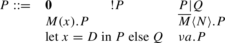
In our calculus terms take up the role of data (messages), while processes (following the grammar in Fig. 1) model functional behavior. $0$ is a process that does nothing, $! P$ (pronounced “bang P”) is an unbounded number of copies of P, $P | Q$ is P and Q in parallel, $M (x)$ waits for a message on channel M and assigns it to x, $\overline{M} ⟨ N ⟩$ outputs N on channel M, $let x = D in P else Q$ evaluates the destructors in D, assigns the result to x and continues with P (or Q if a destructor fails). A signature Σ consists of function symbols which we split in constructors and destructors. A term is either a name, a variable or the application of a constructor to terms. We define the semantic of terms in two ways: One is the equational theory which induces equivalence classes on the set of terms and is defined by set of equations E. The other is a set of rewrite rules R defining the mechanics of destructors. Each rule defines the result of a specific application of a destructor. We call the entity of a signature, a set of equations and a set of rewrite rules a symbolic model. Except for Section 9, it will be clear from the context which symbolic model we use. In Section 9 we focus on the relation between different symbolic models. Only then we will introduce a notation that explicitly states the symbolic model underlying a property, e.g., observational equivalence of two processes.

With $fn (P)$ , $bn (P)$ , $fv (P)$ , $bv (P)$ we denote the free names, bound names, free variables and bound variables of a process, respectively. Analogously $fn (T)$ , $fv (T)$ for terms T. We introduce the usual relations on processes: structural equivalence (≡), internal reduction ( $P \to P^{'}$ ) means that $P^{'}$ is the immediate successor process of P in an execution and observational equivalence (≈) which intuitively means that no context can distinguish the two processes. $D ⇓ M$ means that the destructor term D evaluates to the term M.

2.1. Additional concepts used in this work

In this section, we describe several nonstandard concepts related to the applied pi calculus that we use in this work.

Miscellaneous. A context always contains a single occurrence of the hole. Sometimes we need a context which may or may not contain a hole: A 0–1-context is defined like a context, except that there may be zero or one occurrences of the hole.

We refer to occurrences of terms that identify channels in a process as channel identifiers. E.g., in $\overline{M} ⟨ T ⟩$ M is a channel identifier and T is not – even if M and T were the same term (because M and T are different occurrences).

We allow destructors with conditional rewrite rules following [18], see Appendix B in the Supplemental material. None of our results actually require these conditional destructors, though. The reader may safely assume the usual, unconditional definition of destructors.

Natural symbolic models. A number of lemmas in this paper only hold when the symbolic model we use satisfies certain natural conditions. Instead of stating these explicitly each time, we collect all these conditions in the following definition.

Definition 2.1 (Natural symbolic model).

We say a symbolic model is natural if it satisfies the following conditions:

there is a constructor $empty / 0 \in Σ$ ,

a constructor for pairings, denoted $(□, □)$ , is part of the signature Σ,

there is a destructor $equals / 2 \in Σ$ with rewrite rule $equals (x, x) \to x$ and no further rewrite rules that contain $equals$ ,

there are destructors $fst / 1, snd / 1 \in Σ$ with rewrite rules $fst ((x, y)) \to x$ and $snd ((x, y)) \to y$ ,

for all terms T, $T_{1}$ with $fst (T) ⇓ T_{1}$ there exists a term $T_{2}$ with $snd (T) ⇓ T_{2}$ and furthermore $(T_{1}, T_{2}) =_{E} T$ for all such $T_{2}$ and vice versa,

for arbitrary terms $T_{1}$ , $T_{2}$ , $T_{1}^{'}$ , $T_{2}^{'}$ we require that $(T_{1}, T_{2}) =_{E} (T_{1}^{'}, T_{2}^{'})$ entails $T_{1} =_{E} T_{1}^{'}$ and $T_{2} =_{E} T_{2}^{'}$ ,

for any destructor term D and any name $n \notin fn (D)$ we require that $D ⇓ T$ for a term T entails the existence of a term $T^{'}$ with $D ⇓ T^{'}$ , $n \notin fn (T^{'})$ and $T =_{E} T^{'}$ ,

there are terms T, $T^{'}$ with $T \neq_{E} T^{'}$ .

In the following, we will always assume that the symbolic model is natural in the sense of Definition 2.1.

Equivalence of processes modulo rewriting. Structural equivalence ≡ does not allow us to replace a term M by another term $M^{'} =_{E} M$ . In some places, we will therefore need to apply $=_{E}$ to processes, and we will also use an extension $\equiv_{E}$ of ≡ that allows us to replace terms.

Definition 2.2.
We extend $=_{E}$ to destructor terms and processes as follows:

Given two destructor terms D, $D^{'}$ , we have $D =_{E} D^{'}$ iff D can be rewritten into $D^{'}$ by replacing subterms by $=_{E}$ -equivalent subterms. (But replacing destructors is not allowed.) E.g., if d is a destructor and f, g are constructors, and $f (x) =_{E} g (x)$ is in the equational theory, we have $d (f (a)) =_{E} d (g (a))$ but not $f (d (a)) =_{E} g (d (a))$ . Formally, $=_{E}$ is the smallest equivalence relation on destructor terms such that $D {M / x} =_{E} D {M^{'} / x}$ for destructor terms D and terms $M =_{E} M^{'}$ .

Given two processes P, $P^{'}$ , we have $P =_{E} P^{'}$ iff P can be rewritten into $P^{'}$ by α-conversion and by replacing terms and destructor terms by $=_{E}$ -equivalent ones. Formally, $=_{E}$ is the smallest equivalence relation closed under α-renaming such that $P {M / x} =_{E} P {M^{'} / x}$ for processes P and terms $M =_{E} M^{'}$ .

Given two processes P, $P^{'}$ , we have $P \equiv_{E} P^{'}$ iff P can be rewritten into $P^{'}$ by $=_{E}$ and ≡. Formally, $\equiv_{E} : = {(=_{E} \cup \equiv)}^{}$ .

Full observational equivalence.* A substitution σ is a closing substitution for P if $P σ$ is closed. We call two (not necessarily closed) processes P and Q fully observationally equivalent (denoted $P ≋ Q$ ) iff $P σ \approx Q σ$ for all closing substitutions σ (where we implicitly assume that the bound names in P, Q are renamed so that they are distinct from the free names of σ). Since ≈ is closed under ≡ it follows in a straightforward way that ≋ is closed under ≡.

The motivation behind the definition of ≋ is the following lemma which allows us to replace fully observationally equivalent subprocesses by each other.
Lemma 2.3.
Let P and Q be processes and $P ≋ Q$ . Then $C [P] ≋ C [Q]$ for every context $C$ .

Product processes. In order to argue about concurrent composition, as a technical tool, we will need an extension of the applied pi calculus that supports infinite parallel compositions of processes which are tagged with distinct terms.

Intuitively, the indexed replication $\prod_{x \in S} P$ stands for $P {s_{1} / x} | P {s_{2} / x} | \dots$ when $S = {s_{1}, s_{2}, \dots}$ . (Like $! P$ stands for $P | P | \dots$ .) We call processes from this extended calculus product processes. Note that our main definitions and results are still stated with respect to the original calculus from [7]; we only use product processes in some specific situations.
Definition 2.4 (Product processes).

Product processes are defined by the grammar in Fig. 1 with the additional construct $\prod_{x \in S} P$ where x is a variable, S a (possibly infinite) set of terms, and P a product process. (We call $\prod_{x \in S} P$ an indexed replication.)

(Note that we consider $\prod_{x \in S}$ to be a binder. I.e., in $\prod_{x \in S} P$ , we consider x a bound variable.)

Structural equivalence (≡) on product processes is defined as on processes.

The reduction relation → on product processes is defined using the same rules as on processes, with the following additional rule (IREPL): If $M \in S$ , then $\prod_{x \in S} P \to (\prod_{x \in S^{'}} P) ∣ P M / x$ with $S^{'} : = S ∖ {M^{'} : M =_{E} M^{'}}$ . (Essentially S is treated as a set of session ids which contains each sid at most once modulo $=_{E}$ .)

Observational equivalence (≈) on product processes is defined like observational equivalence on processes.

Notice that processes are also product processes, and that on processes, the new definitions of ≡, →, and ≈ coincide with the original definitions. (See the Supplemental material (Appendix B) for precise definitions.)

3. Useful properties of the pi calculus

In this section, we introduce a number of useful lemmas for the applied pi calculus. These lemmas are useful to derive observational equivalences of processes via step by step rewriting (and for using Proverif as a tool in deriving equivalences that Proverif cannot handle). We believe that they may be useful in other similar situations, too. All proofs can be found in the Supplemental material (Appendix D). Although those lemmas turn out to be quite useful in particular when showing that a concrete protocol emulates another protocol (see, e.g., the proofs of the results in Section 8 and in Section 9), their usefulness may not be obvious at first reading. Thus, the reader may skip this section at first reading. We recommend to simply keep in mind that these lemmas are available and to refer to this section when performing a concrete proof of observational equivalence between two processes.

Lemma 3.1.
For natural symbolic models, the following hold:
If $n \notin fn (M)$ , then $n \neq_{E} M$ .

$n \neq_{E} m$ for names $n \neq m$ .

$(n, M^{'}) \neq_{E} M$ for all terms M, $M^{'}$ and names $n \notin fn (M)$ .

Lemma 3.2.
Let P, $P^{'}$ be processes. Let D, $D^{'}$ be destructor terms. Let M, $M^{'}$ be terms.
If $a \notin fn (P)$ , then $P ≋ ν a . P$ .

If $a \notin fn (M)$ , then $ν a . M (x) . P ≋ M (x) . ν a . P$ .

Assume P is closed and that P does not contain unprotected 3
³
We call an occurrence of an input/output within a process unprotected if it is only below parallel compositions ( $Σ_{}$ ) and restrictions (ν), i.e., it can be executed “right away”.

inputs or outputs. Assume $P \to P^{'}$ , and that for all $P^{″}$ with $P \to P^{″}$ we have $P^{'} \approx P^{″}$ . Then $P \approx P^{'}$ .

If M, $M^{'}$ are terms with $M =_{E} M^{'}$ , then $P {M / x} ≋ P {M^{'} / x}$ .

If for all substitutions σ that close D, M we have $D σ ⇓ M σ$ , and for all $M^{'}$ with $D σ ⇓ M^{'} σ$ we have $M σ =_{E} M^{'} σ$ , then $(let x = D in P else P^{'}) ≋ P {M / x}$ .

If D is closed and there is no M with $D ⇓ M$ , then $(let x = D in P else P^{'}) ≋ P^{'}$ .

If for all substitution σ that close D, $D^{'}$ there exist M, $M^{'}$ with $D σ ⇓ M σ$ , $D^{'} σ ⇓ M^{'} σ$ and $M σ =_{E} M^{'} σ$ then $(if D = D^{'} then P else P^{'}) ≋ P$ .

We have $! P \approx P ∣! P$ .

$\prod_{x \in SID} P \approx \prod_{x \in SID ∖ {t_{1}, \dots, t_{n}}} P | P {\frac{t_{1}}{x}} | \dots | P {\frac{t_{n}}{x}}$ for $t_{1}, \dots, t_{n} \in SID$ .

Lemma 3.3.
Let C be a 0–1-context whose hole is not under a bang and such that n does not occur in C, Q or t. Assume that C does not bind any of $fv (Q) ∖ {x}$ or $fn (Q)$ over its hole. Then $ν n . C [\overline{n} ⟨ t ⟩] | n (x) . Q ≋ C [Q {t / x}]$ .
Lemma 3.4.
Let C, D be contexts, Q a process, n, m names, t, $t^{'}$ terms, and x a variable. Assume that C, D have no bang over their holes. Assume that $n, m \notin fn (C, D, Q, t, t^{'})$ . Assume that C, D do not bind n, m, $fn (Q)$ . Assume that $fv (Q) \subseteq {x}$ .

Then $ν n . (C [! \overline{n} ⟨ t ⟩] ∣ D [n (x) . Q]) \approx ν m . (C [m () . Q {t / x}] ∣ D [\overline{m} ⟨ t^{'} ⟩])$ .
Lemma 3.5.
Let A, B, C be closed processes. If $A \equiv_{E} B \to C$ , then there is a closed process $B^{'}$ such that $A \to B^{'} \equiv_{E} C$ .

3.1. Relating events and observational equivalence

For stating Lemma 3.7 below, we will need processes containing events. The variant of the applied pi calculus presented in Section 2 (which is used by Proverif for observational equivalence proofs) does not support events. When using Proverif for showing trace properties defined in terms of events, a different variant of the applied pi calculus is used [6]. We will call processes in that calculus event processes. Syntactically, event processes differ from processes as in Section 2 only by an additional construct $event f (t_{1}, \dots, t_{n}) . P$ which means that the event f is raised, with arguments $t_{1}, \dots, t_{n}$ (these are normal terms), and then the event process P is executed.

The semantics of event processes are formulated in [6] in a different way from the semantics used here. Fortunately, we will be able to encapsulate everything that we need to know about that semantics in Lemma 3.6 below, so we do not need to repeat those semantics here.

Instead, we extend the definition of the internal reduction relation → to event processes. → is defined as usual, except that we add the following rule: $\begin{matrix} EVENT : event f (t_{1}, \dots, t_{n}) . P \to P \end{matrix}$ The semantics defined by → will be related to those from [6] by Lemma 3.6 below. Event contexts are contexts that additionally contain events, and evaluation event contexts are evaluation contexts that additionally contain events, but not over their hole.

Finally, [6] defines the concept of a trace property. We will only need trace properties of a specific form, namely $\begin{matrix} end (x) ⟹ start (x) \lor x = t_{1} \lor \dots \lor x = t_{n} \end{matrix}$ Intuitively, an event process P satisfies a trace property $end (x) \Rightarrow start (x) \lor x = t_{1} \lor \dots \lor x = t_{n}$ if in any execution $P | R \to P_{1} \to \dots \to P_{n}$ , we have that if one of the transitions raises the event $end (t)$ , then $t \in {t_{1}, \dots, t_{n}}$ or in the same trace, the event $start (t)$ is also raised (for any adversarial R not containing events).

Formally, satisfying a trace property is defined with respect to the semantics from [6].4

⁴
Strictly speaking, the semantics described in [6] does not allow expressions of the form $x = t_{i}$ in trace properties. Such expressions are, however, supported by Proverif. Also, [6, footnote 3 in the full version] explains how to encode such equality tests in the trace properties supported by [6]. In their notation, our trace property becomes the somewhat less readable trace property: $end (x) \Rightarrow (end (x) ⇝ start (x)) \lor (end (t_{1}) ⇝ true) \lor \dots \lor (end (t_{n}) ⇝ true)$ .

Also, the semantics described [6] do not support equations (i.e., $t =_{E} t^{'}$ iff $t = t^{'}$ in their semantics). However, Proverif supports these, so we assume the intended semantics of Proverif is that of [6] with the natural extension of equality tests to equality modulo $=_{E}$ .

Instead of giving those semantics here, we present the following lemma which summarizes seven facts about that definition. We will not use any other facts. The facts can be verified by inspecting the semantics and definitions from [6].

Lemma 3.6.

Let $t_{1}, \dots, t_{n}$ be terms. Let ℘ stand for the trace property $end (x) \Rightarrow start (x) \lor x = t_{1} \lor \dots \lor x = t_{n}$ . Let P be an event process.

If $P \equiv P^{'}$ and P satisfies ℘, then $P^{'}$ satisfies ℘ .

Assume $P \to P^{'}$ and P satisfies ℘ and the reduction $P \to P^{'}$ does not use the EVENT rule. Then $P^{'}$ satisfies ℘ .

Let t be a closed term. Assume $P = C [event start (t) . Q]$ where C is an event context not binding $fn (t)$ over its hole. Assume that P satisfies ℘. Then $P^{'} : = C [Q]$ satisfies $℘ \lor x = t$ .

Assume $P = C [event end (t) . Q]$ where C is an event context. Assume that P satisfies ℘. Then $P^{'} : = C [Q]$ satisfies ℘ .

Assume P satisfies ℘ and E is an evaluation context (not containing events) and E does not bind $fn (t_{1}, \dots, t_{n})$ over its hole. Then $E [P]$ satisfies ℘ .

Assume E is an evaluation event context that does not bind any names over its hole. Assume $P = E [event end (t) . Q]$ . Assume that P satisfies ℘. Then $t =_{E} t_{i}$ for some i.

If $ν a . P$ satisfies ℘, then P satisfies ℘ .

We explain the intuitive reason for each fact:

Structurally equivalent processes behave identically and thus raise the same events.

If $P \to P^{'}$ without raising an event, then for any event trace that $P^{'}$ may produce, P may produce the same by first reducing to $P^{'}$ .

$P^{'}$ has the same event traces as P, except that some $start (t)$ -events are removed. If $P^{'}$ does not satisfy $℘ \lor x = t$ , then there must be an event $end (t^{'})$ with $t \neq t^{'}$ that is not preceded by a $start (t^{'})$ -event. But then also in a trace of P, there would be an $end (t^{'})$ -event not preceded by $start (t^{'})$ (since the traces only differ in their $start (t)$ -events and $start (t) \neq start (t^{'})$ ).

$P^{'}$ has the same event traces as P, except that various $end (\cdot)$ -events are removed. (Since t is not necessarily closed, $end (t)$ may be instantiated to different $end (\cdot)$ -events.) If a trace of $P^{'}$ does not satisfy ℘, this means there was an $end (t^{'})$ -event not preceded by a $start (t^{'})$ event. Then also in P the corresponding $end (t^{'})$ -event is not preceded by a $start (t^{'})$ -event, as P has the same $start (\cdot)$ -events, and more $end (\cdot)$ -events.

The semantics of satisfying trace properties are defined with respect to P running in parallel with an adversary R not containing events. Thus the case of an evaluation context running with P is already covered. (It is important that E does not bind $fn (t_{1}, \dots, t_{n})$ because otherwise the terms $t_{1}, \dots, t_{n}$ occurring in the process would be considered different from those in ℘.)

There is a trace of P that consists only of an $end (t)$ -event. That trace does not satisfy $end (t) \Rightarrow start (t)$ . Thus it satisfies ℘ only if ℘ contains $x = t$ as one of its clauses.

$ν a . P$ has the same traces as P, except that occurrences of a in the P-traces are replaced by a fresh restricted name $a^{'}$ . Thus, if P does not satisfy ℘, then there is a trace containing an $end (t)$ -event without preceding $start (t)$ -event such that $t \notin {t_{1}, \dots, t_{n}}$ . In the corresponding $ν a . P$ -trace, we have an $end (t {a^{'} / a})$ -event without preceding $start (t {a^{'} / a})$ -event. Since $t \notin {t_{1}, \dots, t_{n}}$ and a is fresh, also $t {a^{'} / a} \notin {t_{1}, \dots, t_{n}}$ . Hence the $ν a . P$ -trace does not satisfy ℘, either.

Lemma 3.7.

Let s be a name. Let P be a process containing the subterm s only in constructs of the form $(! \overline{(s, t)} ⟨ t^{'} ⟩) | P^{'}$ and $(s, t) () . P^{'}$ (for arbitrary and possibly different t, $t^{'}$ , $P^{'}$ ) .

Let ${plain}^{s} (P)$ denote the process resulting from P by replacing all occurrences $! \overline{(s, t)} ⟨ t^{'} ⟩ | P^{'}$ and $(s, t) () . P^{'}$ by $P^{'}$ .

Let ${ev}^{s} (P)$ denote the process resulting from P by replacing all occurrences $! \overline{(s, t)} ⟨ t^{'} ⟩ | P^{'}$ by $event start (t) . P^{'}$ and $(s, t) () . P^{'}$ by $event end (t) . P^{'}$ .

Assume that ${ev}^{s} (P)$ satisfies the trace property $end (x) \Rightarrow start (x)$ .

Then ${plain}^{s} (P) \approx ν s . P$ .

Lemma 3.8 (Unpredictability of nonces).

Let C be a context not binding the variable x and let P, Q be processes. Then $ν r . C [if x = r then P else Q] ≋ ν r . C [Q]$ .

4. Symbolic UC

Intuition. We start by presenting the intuition that underlies the original UC framework [9] and thus also our work. The basic idea is to define security of a protocol π by comparing it to a so-called ideal functionality $F$ . The ideal functionality is a machine that by definition does what the protocol should achieve. For example, if the task of the protocol is to transmit a message m securely from Alice to Bob, then the functionality is a trusted machine that expects a message m from Alice over a secure channel, sends to the adversary that such a message was received (but does not send the message itself), and then after the adversary allows delivery, forwards the message to Bob. (In the applied pi calculus, this functionality would be ${net}_{scstart} () . {io}_{A} (x) . (\overline{{net}_{notify}} ⟨ ⟩ ∣ {net}_{deliver} () . \overline{{io}_{B}} ⟨ x ⟩)$ where the ${net}_{\dots}$ -channels belong to the adversary; see Definition 6.2 below.) In a sense, the functionality is an abstract specification of the protocol behavior, and the protocol is supposed to be a concrete instantiation of that specification using crypto, in a way that preserves the security properties of the specification.

So how to model that a protocol π is as secure as a functionality $F$ ? The basic idea is to ensure that any attack on π is also possible on $F$ . Since by assumption $F$ does not allow any attacks, this implies that π does not allow any attacks either, so π is secure. To model that any attack on π is possible on $F$ , we require that for any adversary attacking π, there is a corresponding adversary (the “simulator”) attacking $F$ that performs an equivalent attack. And what do we mean by equivalent? Any “environment” that can observe the overall protocol outcome (inputs and outputs), and that can talk to the adversary (i.e., it learns what secret information the adversary might have obtained), cannot distinguish between the two attacks. In other words, for any adversary A, there is a simulator S such that for all environments Z, we have that $π + A + Z$ (the protocol running with A and Z) and $F + S + Z$ are indistinguishable from Z’s point of view. Notice that we do not wish to allow Z to observe the internal protocol communication – doing so would require that π and $F$ work the same way internally, but we only want that the two have the same “observable effects”, we do not care about their inner workings. Due to this, in a formal definition, we need to distinguish between the protocol-internal communication channels (net-channels), and the protocol’s interface (io-channels). Only the latter is accessible to the environment.

Formal definition. To formalize the above intuition in the applied pi calculus, we first formalize the distinction between channels that make up the protocol’s input/output interface, and those that make up the protocol’s internal channels. We partition the set of all names into two sets $IO$ and $NET$ (both infinite). We will then require adversaries and simulators to only communicate on $NET$ channels. (We do not forbid the environment to access $NET$ channels. But we will give the adversary/simulator the ability to rename and hide $NET$ channels, and thus effectively protect the protocol’s $NET$ channels from the environment.)

In order to keep the distinction between NET-channels and IO-channels, we also want to avoid that NET-channels are transmitted to the environment (we use this in a few places in our proofs).

Definition 4.1.
We call a process P $NET$ -stable if every name $n \in NET \cap fn (P)$ in P occurs only in channel identifiers (i.e., in particular, P does not send n to the environment).

Note that there is no restrictions on the bound names. Thus a $NET$ -stable adversary is free to share arbitrary fresh names with the environment and to use them as channels.

We now define the concept of an adversary. Essentially, an adversary is just a process A that is intended to interact with the protocol (or functionality). Since the adversary connects to the protocol over some $NET$ -names, the specification of the adversary additionally includes a list of NET-names $\underline{n}$ of the protocol that will be accessed by A (and are thus private between A and the protocol). Finally, an adversary/simulator sometimes needs to rename NET-channels of the protocol/functionality to avoid name clashes. Since NET-channels are protocol internal and not part of the externally visible interface, it should not matter whether the same name is used in protocol and functionality or not. This is achieved by letting the adversary rename NET-names, we model this by specifying a renaming φ as part of the adversary.
Definition 4.2.
An adversary is a triple $(A, φ, \underline{n})$ where A is a closed $NET$ -stable process with $IO \cap fn (A) = \emptyset$ , $φ : NET \to NET$ a bijection and $\underline{n}$ a list of names $\underline{n} \subseteq NET$ .

We can now state our security definition. Both protocol and functionality are modeled by processes P and Q, respectively. An adversary $(A, φ_{A}, {\underline{n}}_{A})$ connecting to P is modeled as $ν {\underline{n}}_{A} . (P φ_{A} | A)$ , as we would expect from the meaning of φ and $\underline{n}$ explained above. To model that P emulates Q, we would require that $ν {\underline{n}}_{A} . (P φ_{A} | A)$ and $ν {\underline{n}}_{S} . (Q φ_{S} | S)$ are indistinguishable for any environment for a suitable simulator $(S, φ_{S}, {\underline{n}}_{S})$ . We do not need to specify the environment explicitly because we have the notion of observational equivalence: $ν {\underline{n}}_{A} . (P φ_{A} | A) \approx ν {\underline{n}}_{S} . (Q φ_{S} | S)$ means that no context can distinguish the left- and right-hand side. The following definition captures this, except that we make one simplification: Instead of quantifying over all adversaries $(A, φ_{A}, {\underline{n}}_{A})$ , we fix $A : = 0$ , $φ_{A}$ the identity, and ${\underline{n}}_{A}$ the empty list, so that $ν {\underline{n}}_{A} . (P φ_{A} | A) = P$ . (Such an adversary, that essentially just leaves all NET-channels accessible to the environment, is usually called a dummy adversary.) This definition is often technically much simpler to handle, and Lemma 4.4 below guarantees that it is equivalent to the more natural definition that quantifies over all adversaries.
Definition 4.3.
Let P and Q be processes. We say P emulates Q (written $P ⩽ Q$ ) iff there exists an adversary $(S, φ, \underline{n})$ such that $P ≋ ν \underline{n} . (Q φ | S)$ . $(S, φ, \underline{n})$ will often be called simulator.

We use ≋ instead of ≈ to get a more general definition, allowing non-closed P, Q. For the applications presented in this paper, the special case using ≈ (which is equivalent to our definition restricted to closed processes) is sufficient. (Note however that we would still use ≋ to state various technical lemmas more conveniently.)

Note that there is no formal distinction between protocols and functionalities. Indeed, it can sometimes be convenient to compare two protocols P, Q. Furthermore, note that ⩽ is weaker than ≋: $P ≋ Q$ entails $P ⩽ Q$ (and $Q ⩽ P$ ) with the simulator $(0, id, \emptyset)$ .

As observed in [24] there are several approaches to define simulation based security. The following Lemma shows that our definition (resembling strong simulatability ) is equivalent to the two alternatives: black-box simulatability and universally-composable simulatability (the latter being the definition that corresponds directly to the intuition given at the beginning of this section).
Lemma 4.4.
For processes P, Q we have that the following are equivalent:
strong simulatability: $P ⩽ Q$ ,

black-box simulatability: $\exists (S, φ_{S}, {\underline{n}}_{S})$ $\forall (A, φ_{A}, {\underline{n}}_{A}) ν {\underline{n}}_{A} . (P φ_{A} | A) ≋ ν {\underline{n}}_{A} . ((ν {\underline{n}}_{S} . (Q φ_{S} | S)) φ_{A} | A)$ ,

universally-composable simulatability: $\forall (A, φ_{A}, {\underline{n}}_{A})$ $\exists (S, φ_{S}, {\underline{n}}_{S}) ν {\underline{n}}_{A} . (P φ_{A} | A) ≋ ν {\underline{n}}_{S} . (Q φ_{S} | S)$ ,

where all triples are adversaries according to Definition 4.2 .
Lemma 4.5 (Reflexivity, transitivity).

Let P, Q, R be processes. Then $P ⩽ P$ . And if $P ⩽ Q$ and $Q ⩽ R$ , then $P ⩽ R$ .

Corruption. So far, we have not yet modeled the ability of the adversary to corrupt parties. There are two main variants of corruption: static and adaptive corruption. In the case of static corruption, it is determined in the beginning of the protocol who is corrupted. For adaptive corruption, corruption may occur during the protocol and depend on protocol messages. Modeling static corruption is quite easy in our model: When a party X is corrupted, we simply remove the subprocess $P_{X}$ corresponding to that party from the protocol P, make all NET-names occurring in $P_{X}$ public, and – in the case of a functionality – additionally rename all IO-names of $P_{X}$ into NET-names. For example, if $P = ν {net}_{1} {net}_{2} . (P_{A} | P_{B} | F)$ where ${net}_{1}$ occurs in $P_{A}$ and $P_{B}$ and ${net}_{2}$ only in $P_{B}$ , and $F$ has IO-names ${io}_{FA}$ , ${io}_{FB}$ then corrupting A leads to $P^{'} = ν {net}_{2} . (P_{B} | F {{net}_{FA} / {io}_{FA}})$ . And a functionality $G$ with IO-names ${io}_{A}$ , ${io}_{B}$ becomes $G {{net}_{A} / {io}_{A}}$ .

So, if we want to verify that a P emulates $G$ for any corruption, we need to check:

Uncorrupted: $P ⩽ G$ .

Alice corrupted: $ν {net}_{2} . (P_{B} | F {{net}_{FA} / {io}_{FA}}) ⩽ G {{net}_{A} / {io}_{A}}$ .

Bob corrupted: $P_{A} | F {{net}_{FB} / {io}_{FB}} ⩽ G {{net}_{B} / {io}_{B}}$ .

An example is given in Section 9.1 in the case of UC secure commitments.

Modeling adaptive corruptions is more complex. For this one would need to introduce special parties that react to a special signal from the environment and then switch into a corrupted mode. We do not follow that approach here.

Comparison with computational UC. We quickly highlight a few differences between our symbolic UC model and the computational UC model from [9]. The most obvious difference is, of course, that in our model messages are terms, while in the computational UC model messages are bitstrings. And the adversary’s capabilities in our model are specified by the equational theory and the destructors, while in the computational UC model, the adversary can perform any probabilistic polynomial-time computation. Also, nonces are modeled via fresh names in our model (and thus in principle unguessable), while nonces would be realized by hard to guess (but not impossible to guess) random bitstrings in the computational UC model. Our model does not allow to model probabilism (i.e., if we would design a protocol where an attack is possible with very small probability, our model would consider that protocol totally insecure).

Besides that, there are a number of smaller differences: Scheduling decisions (e.g., when two messages are sent at the same time) are non-deterministic in our model while in computational UC, the scheduling is determined by the adversary. The computational UC model does not know the concept of a blocking output (i.e., when sending a message, the recipient cannot influence the sender by not accepting the message), while in our model we have both blocking ( $\overline{n} ⟨ x ⟩ . P$ ) and non-blocking ( $\overline{n} ⟨ x ⟩ | P$ ) outputs.5

⁵
However, we find that security proofs get harder when actually making use of the blocking outputs in our protocols and functionalities. See our guideline on p. 21.

The computational UC model has a built-in framework for distinguishing parallel-composed processes using session-ids while in our model we need to work hard to mimic those session-ids (see the next section). We believe, however, that none of these differences are crucial for building a symbolic UC variant. They simply result from using the applied π-calculus as our underlying calculus. We could as well have chosen to model our symbolic UC model to mimic the computational UC model in every respect except for the fact that the messages are symbolic.6

⁶

That is, we could go through the definition of the computational UC framework and essentially replace the machine model from Turing machines to machines that operate on terms and not change much else.

(Note that the converse does not hold: we do not see how to add non-determinism to a computational UC model because non-determinism and probabilism do not easily interact.)

5. Composition

One of the salient properties of the UC framework is composition. Assume a protocol π UC-emulates a functionality $F$ . And ρ is a protocol using $F$ . Then $ρ^{π / F}$ (which is ρ with $F$ replaced by π) UC-emulates ρ. And hence, by transitivity, if ρ emulates some functionality $G$ , $ρ^{π / F}$ UC-emulates $G$ .

In our context, ideally we would like a composition theorem such as $P ⩽ Q \Rightarrow C [P] ⩽ C [Q]$ for arbitrary contexts C. Unfortunately, the situation is not as simple. A simple observation is that if C may contain NET-names, then composition will not work: For example, assume $P ⩽ Q$ , and P is a protocol using some NET-channel $net$ to implement an ideal functionality Q (which does not use $net$ ). And $C = □ | R$ receives on a NET-channel $net$ and outputs the received messages on an IO-channel $io$ . Then $C [P]$ will output protocol-internal messages on $io$ (observable to the environment), while $C [Q]$ will not (since the functionality Q will not use the channel $net$ ). Hence $C [P] ⩽̸ C [Q]$ . We give a formal analysis of the various cases in which the composition theorem does not hold in Appendix A.

Thus a first condition on C is that it may not use the same NET-names. In fact, we show below (Theorem 5.10) that if C is an evaluation context binding only IO-names and not using any of the NET-names of P, Q, then $P ⩽ Q \Rightarrow C [P] ⩽ C [Q]$ holds.

This already allows for a large range of composition operations. (In particular, we can connect different protocols through their interfaces securely by composing them in parallel, and restricting the IO-channels through which they are connected.) But one important operation is missing, namely concurrent composition. Concurrent composition means that if $P ⩽ Q$ , then $P^{'} ⩽ Q^{'}$ where $P^{'}$ consists of many instances of P and $Q^{'}$ analogously. Such a result is important in many cases, e.g., if P is a single session key-exchange, but an embedding protocol needs a large number of keys. The most obvious way to model this in our setting would be a theorem stating $P ⩽ Q \Rightarrow! P ⩽! Q$ .

Unfortunately, such a theorem cannot hold, either. The intuitive reason is as follows: When trying to construct a simulator for $! Q$ , then this simulator will not be able to distinguish messages from different instances of Q. The simulator will then be unable to even decide whether he talks to a single instance or several. For example: $\begin{array}{rcl} P : = ν n m . (\overline{{io}_{1}} ⟨ n ⟩ ∣ {io}_{2} (x) . if x = n then \overline{{net}_{2}} ⟨ m ⟩ \\ ∣ {io}_{3} (x) . if x = n then \overline{{net}_{3}} ⟨ m ⟩) \\ Q : = ν n . (\overline{{io}_{1}} ⟨ n ⟩ ∣ {io}_{2} (x) . if x = n then \overline{{net}_{2}} ⟨ empty ⟩ \\ ∣ {io}_{3} (x) . if x = n then \overline{{net}_{3}} ⟨ empty ⟩) \end{array}$ Here we have $P ⩽ Q$ because a simulator receiving $empty$ on ${net}_{2}$ or ${net}_{3}$ just has to replace it by some fresh name m. However, we do not have $! P ⩽! Q$ . Depending on the messages the environment sends on ${io}_{2}$ , $! P$ will output either the same name m on ${net}_{2}$ , ${net}_{3}$ , or different names m, $m^{'}$ . However, a simulator interacting with $! Q$ in both cases gets $empty$ , $empty$ on ${net}_{2}$ , ${net}_{3}$ . The simulator then does not know whether he should change this into m, m or m, $m^{'}$ for fresh m, $m^{'}$ . Thus the simulator fails. (The formal argument is in Appendix A.)

So we cannot have a theorem stating $P ⩽ Q \Rightarrow! P ⩽! Q$ . Does this mean concurrent composition is not possible? No, just that ! is not the right operator to model it. In the computational UC framework, composition also does not involve a number of indistinguishable instances. Instead, each instance of P and Q is given a unique session id, and all communication is tagged with that session id so that it can be routed to the right instance. In our setting, one possibility to achieve this is to define an operator $!!$ [17] such that $!! P$ behaves like an unlimited number of instances of P, where each instance is tagged with a unique session id $sid$ . I.e., each channel C in P is replaced by $(sid, C)$ .7

⁷
One might instead consider tagging the messages sent over the channel with $sid$ . This, however, does not work as well: One would need a specific multiplexer process that given a message $(sid, T)$ discovers the corresponding instance of P and delivers to it. This might be possible, but is probably considerably more complicated than the approach we take further.

The question is how to define $!! P$ . The applied pi calculus does not have any construct that conveniently allows to perform infinite branching with different ids. Thus, we have to work around this restriction by introducing a more elaborate construction. As a first step, we define the tagged version $P ((M))$ of the process P in the following definition.

Definition 5.1.

Let P be a process, and let M be a term. We write $P ((M))$ for P with every occurrence of $C (x)$ replaced by $(M, C) (x)$ and every occurrence of $\overline{C} ⟨ T ⟩$ replaced by $\overline{(M, C)} ⟨ T ⟩$ . (If M contains bound variables or bound names from P, we assume that these bound variables/names are first renamed in P.)

Now we have to somehow define $!! P$ as $P ((s_{1})) | P ((s_{2})) | \dots$ where $s_{1}, s_{2}, \dots$ range over some infinite set $SID$ of session ids. Using product processes (see Section 2.1) this is easy: $!! P : = \prod_{x \in SID} P ((x))$ does the job. However, product processes are a nonstandard extension of the applied pi calculus, but we wish to stay compatible with existing variants (in particular, to be able to use Proverif for verification). Thus, instead of using $\prod_{x \in SID} P ((x))$ , we define a suitable context $C$ such that $C [P ((x))]$ behaves like $\prod_{x \in SID} P ((x))$ . Then we can define $!! P : = C [P ((x))]$ . Of course, depending on the particular set $SID$ we choose, a different context $C$ will be needed. Instead of fixing a particular one, we thus give a general definition what contexts are suitable for a given set $SID$ , and from then on, just assume an arbitrary such context.

Definition 5.2 (Indexing context).

Given a set S of terms, a variable x (will be used for tagging), and names $\underline{n}$ , we call a closed context $C_{x, \underline{n}}$ with $bn (C_{x, \underline{n}}) = \underline{n}$ and $fn (C_{x, \underline{n}}) = \emptyset$ (not containing indexed replications) an S-indexing context iff for all processes P with $x \notin bv (P)$ 8

⁸
P may have $x \in fv (P)$ but we forbid $x \in bv (P)$ to avoid technicalities in the definition of $P ((x))$ due to the shadowed x.

and

\underline{n} \cap fn (P) = \emptyset

we have

\begin{matrix} C_{x, \underline{n}} [P ((x))] ≋ \prod_{x \in S} P ((x)) \end{matrix}

In the following, we fix a set $SID$ of terms containing no names or variables. The set $SID$ will represent the set of all session IDs. We assume that $id =_{E} {id}^{'}$ entails $id = {id}^{'}$ for $id, {id}^{'} \in SID$ (different IDs are never equivalent by the equational theory).

Note that not for every set $SID$ a $SID$ -indexing context exists. For example, if $SID$ is not semi-decidable (but the equational theory is), then there is no $SID$ -indexing context. One might be concerned that our definition of $SID$ -indexing contexts cannot be fulfilled. The following definition shows that this is not the case, at least if we use suitably encoded bitstrings as SIDs.

Definition 5.3.

Assume that a nullary constructor $nil$ and unary constructors $zero$ and $one$ are part of our symbolic model. Let ${SID}_{bits}$ be the set of all terms built from $nil$ , $zero$ and $one$ . Assume furthermore that for $id, {id}^{'} \in {SID}_{bits}$ in our symbolic model $id =_{E} {id}^{'}$ entails $id = {id}^{'}$ . Let $\begin{matrix} C_{x, a}^{{SID}_{bits}} : = ν a . (\overline{a} ⟨ nil ⟩ |! a (x) . (\overline{a} ⟨ zero (x) ⟩ | \overline{a} ⟨ one (x) ⟩ | □)) \end{matrix}$

Intuitively, $C_{x, a}^{{SID}_{bits}}$ is a factory with parameters xand afor tagged instances of P that realizes the abstract construction of $\prod_{x \in {SID}_{bits}} P ((x))$ . The following lemma formalizes this fact.

Lemma 5.4.

$C_{x, a}^{{SID}_{bits}}$ is an ${SID}_{bits}$ -indexing context.

We stress that $C_{x, a}^{{SID}_{bits}}$ is just one example of an indexing context. From now on $SID$ is an arbitrary but fixed set of indexes and $C_{x, \underline{n}}^{SID}$ an arbitrary but fixed $SID$ -indexing context according to Definition 5.2. All our results then hold independently of the particular choice of $SID$ .

We can now finally define $!! P$ in the following definition.

Definition 5.5 (Indexed replication).

Let P be a process. We define $!!_{x} P : = C_{x, \underline{n}}^{SID} [P ((x))]$ for some arbitrary $\underline{n}$ with $\underline{n} \cap fn (P) = \emptyset$ . We write $!! P$ for $!!_{x} P$ with $x \notin (fv (P) \cup bv (P))$ .

Notice that our definition is a bit more general, we can even write $!!_{x} P$ , in this case P will have access to the sid via the variable x. We need this added flexibility in Section 8.3 for the protocol ${KE}^{*}$ .

Note that since $C_{x, \underline{n}}^{SID} [P ((x))] ≋ \prod_{x \in S} P ((x))$ by definition, we can actually think of $!!_{x} P$ as being defined as $\prod_{x \in S} P ((x))$ . Our definition, however, has the advantage that $!!_{x} P$ is actually a process in the original calculus, the concept of product processes was only used as a tool for defining $!!$ .

On real-life implementations of $!!$ . When implementing a process $!! P$ in real life (i.e., in software for actual deployed protocols), a process such as $!! c (x) . P^{'}$ is probably best implemented by a process that listens on c for messages of the form $(sid, m)$ . Whenever such a message is received, a new instance of $P^{'}$ with session id $sid$ is spawned, and all further messages with that $sid$ are routed to that instance of $P^{'}$ . On the other hand, a process such as $!! \overline{c} ⟨ M ⟩ . P^{'}$ cannot be implemented, because such a process would non-deterministically send $(sid, M)$ for all possible $sid$ . A process $!! (A | B)$ , where A and B correspond to processes run on different computers, does not immediately make sense, because if, e.g., A receives a message that spawns a new instance, B would have to spawn a new instance, too, without communication between A and B. Fortunately, we show in Lemma 5.9 below that $!! (A | B) ≋!! A ∣!! B$ ; then A and B can spawn instances independently. (Note: when we write several occurrences of $!!$ , the implicit set $SID$ is the same for all of them.)

Properties of $!!$ . The following four lemmas state several important properties of $!!$ . We will need these to prove the composition theorem below. Lemmas 5.6, 5.7 and 5.9 also hold for ! instead of $!!$ . But Lemma 5.8 is specific to $!!$ , and is crucial for enabling the composition theorem.

Lemma 5.6.
Let P be a process and $φ : N \to N$ be a permutation on names. Then $(!!_{x} P) φ \equiv!!_{x} (P φ)$ for all variables $x \notin bv (P)$ .
Lemma 5.7.
Let P, Q be processes. Then $P ≋ Q \Rightarrow!!_{x} P ≋!!_{x} Q$ for all variables $x \notin bv (P) \cup bv (Q)$ .
Lemma 5.8.
Let P be a process and n be a name that occurs only in channel identifiers in P. Then $ν n .!!_{x} P ≋!!_{x} ν n . P$ for all variables $x \notin bv (P)$ .
Lemma 5.9.
Let P and Q be processes. Then $!!_{x} (P | Q) ≋!!_{x} P |!!_{x} Q$ for all variables $x \notin bv (P) \cup bv (Q)$ .

Out of these four lemmas, Lemma 5.7 was surprisingly hard to prove. We very roughly sketch the proof idea here: The main thing to show is that $P \approx Q \Rightarrow P ((M)) \approx Q ((M))$ for arbitrary fixed M. To show this, we define an operation $untag$ that maps $P ((M))$ to P, i.e., removes the tag M from all channels. Then we wish to prove that the following relation is a bisimulation: $\sim_{S_{sid}} : = {(P, Q) : untag (P) \approx untag (Q)}$ . Once we have that, we see that $P ((M)) \sim_{S_{sid}} Q ((M))$ and hence $P ((M)) \approx Q ((M))$ . Unfortunately, $\sim_{S_{sid}}$ is not really a bisimulation. A bisimulation must be closed under evaluation contexts, even under contexts in which not all channels are tagged with M. To solve this problem, we tweak $untag$ in such a way that non-tagged channels C are mapped to specially marked channels (using a special name $n_{sid}$ ) which can then be mapped back to C when tagging again. And we need to tweak the notion of a bisimulation slightly, so that $\sim_{S_{sid}}$ only needs to be closed under evaluation contexts on which our operation $untag$ works properly. These tweaks lead to an unexpectedly complex proof of Lemma 5.7.

Alternative definitions of $!!$ . Of course, our definition of $!! P$ is not the only possible definition of a replication with session ids. For example, one might try to define $!! P$ in such a way that an instance of P is spawned for arbitrary terms as sessions id, not only terms in some fixed set $SID$ . In particular, a fresh name could then be used as session id which is not possible with our modeling.9
⁹
One needs to be careful with the following situation, though: If $ν k . Q$ is a process with a secret name k, then $ν k . Q |!! P \equiv ν k . (Q |!! P) \to ν k . (Q |!!^{'} P | P ((k)))$ where $!!^{'} P$ stands for $!! P$ without the session id k. That is, a new process $P ((k))$ has been spawned that “magically” knows the secret name k of Q. One needs to ensure that the name k can never leaks to the outside of $P ((k))$ , e.g., by ensuring that $P ((k))$ only communicates with processes that already know k.

Any definition of $!!$ that satisfies Lemmas 5.6–5.9 would lead to the same composition theorem. (If that definition $!!$ is applicable only to a certain set P of processes, we additionally need that P is closed under parallel composition, restrictions, renaming, and $!!$ , and that the definition of ⩽ (Definition 4.3) is with respect to simulators in P.)

The composition theorem. We can now state and prove the composition theorem. It says that if $P ⩽ Q$ , we can restrict the IO-names, compose in parallel with processes that have disjoint NET-names, rename names (as long as NET- and IO-names are not interchanged), and perform concurrent composition. Theorem 5.10 (Composition theorem).

Let P, Q be processes with $P ⩽ Q$ . Then

For any list of names $\underline{io} \subseteq IO$ we have $ν \underline{i o} . P ⩽ ν \underline{i o} . Q$ .

For any process R with $(fn (R) \cap (fn (P) \cup fn (Q))) \subseteq IO$ we have $P | R ⩽ Q | R$ .

For any permutation $ψ : NET \to NET$ we have $P ψ ⩽ Q$ and $P ⩽ Q ψ$ .

For any permutation $ψ : IO \to IO$ we have $P ψ ⩽ Q ψ$ .

If Q is a $NET$ -stable process, $!!_{x} P ⩽!!_{x} Q$ for all variables $x \notin bv (P) \cup bv (Q)$ .

Proof.
In the following, let $(S, φ, \underline{n})$ be as in Definition 4.3. (They exist because $P ⩽ Q$ .)
$P ≋ ν \underline{n} . (Q φ | S) \overset{()}{\Rightarrow} ν \underline{io} . P ≋ ν \underline{io} . ν \underline{n} . (Q φ | S) \overset{( )}{≋} ν \underline{n} . ((ν \underline{io} . Q) φ | S)$

since ≋ is closed under the application of evaluation contexts;

since neither S nor φ contain names from $IO$ .

W.l.o.g. we can assume $fn (R) \cap \underline{n} = \emptyset$ and that φ is the identity on $(fn (R) \cup bn (R)) \cap NET$ . These assumptions guarantee (∗) in the upcoming equations. $P ≋ ν \underline{n} . (Q φ | S) \Rightarrow P | R ≋ ν \underline{n} . (Q φ | S) | R \overset{()}{≋} ν \underline{n} . ((Q | R) φ | S)$ .

$P ≋ ν \underline{n} . (Q φ | S) \Rightarrow P ψ ≋ (ν \underline{n} . (Q φ | S)) ψ \equiv ν \underline{n} ψ . (Q (ψ \circ φ) | S ψ)$ . Therefore, with $(S ψ, ψ \circ φ, \underline{n} ψ)$ as simulator, we have $P ψ ⩽ Q$ . With $(S, φ \circ ψ^{- 1}, \underline{n})$ we have $P ⩽ Q ψ$ .

$P ≋ ν \underline{n} . (Q φ | S) \Rightarrow P ψ ≋ (ν \underline{n} . (Q φ | S)) ψ \equiv ν \underline{n} . (Q (φ \circ ψ) | S)$ since S, φ and $\underline{n}$ do not contain $IO$ names and thus are not affected by $ψ : IO \to IO$ .

Note that $Q φ$ is $NET$ -stable since Q is $NET$ -stable. Then $P ≋ ν \underline{n} . (Q φ | S)$ entails $\begin{array}{rcl} !!_{x} P & ≋ & !!_{x} ν \underline{n} . (Q φ | S) (by Lemma 5.7) \\ ≋ & ν \underline{n} .!!_{x} (Q φ | S) (by Lemma 5.8 since Q φ | S NET -stable) \\ ≋ & ν \underline{n} . (!!_{x} (Q φ) |!!_{x} S) (by Lemma 5.9) \\ \equiv & ν \underline{n} . ((!!_{x} Q) φ |!!_{x} S) (by Lemma 5.6) \end{array}$ Thus $(!!_{x} S, φ, \underline{n})$ is a proper simulator for $!!_{x} P ⩽!!_{x} Q$ . □

6. Property preservation

Besides secure composition, the second salient property of the UC framework is the fact that security properties of the ideal functionality $F$ automatically carry over to any protocol emulating $F$ . For example, a secure channel functionality that takes a message m from Alice and gives it directly to Bob will obviously have the property that m stays secret. Then, if π UC-emulates $F$ , any message given to π will also stay secret. A similar property preservation law holds in our case, the following theorem formalizes it.

Theorem 6.1 (Property preservation).

Let P, Q be NET-stable processes with $P ⩽ Q$ . Let $E_{1}$ and $E_{2}$ be contexts whose holes are protected only by parallel compositions (|), restrictions (ν), and indexed replications ( $!!_{x}$ ). Assume that $E_{1}$ , $E_{2}$ do not contain NET-names (neither bound nor free). Assume that the number of $!!_{x}$ (possibly with different x) over the hole is the same in $E_{1}$ and $E_{2}$ .

If $E_{1} [Q] ≋ E_{2} [Q]$ , then $E_{1} [P] ≋ E_{2} [P]$ .

Thus, any security property that can be expressed by an indistinguishability game of the form “ $E_{1} [P] ≋ E_{2} [P]$ ” with $E_{1}$ , $E_{2}$ as in the theorem will carry over from the ideal functionality Q to the protocol P, given $P ⩽ Q$ . Note that even many trace based properties can be expressed in such a way. E.g., if we want to say that $E_{1} [P]$ does not raise an event $bad$ (modeled by emitting on a special channel), we just define $E_{2}$ to be like $E_{1}$ , but without the event. Then $E_{1} [P] ≋ E_{2} [P]$ implies that $E_{1} [P]$ does not raise the event.

Example (Strong secrecy).

We illustrate the use of this theorem with an example. Consider the secure channel functionality in the following definition.

Definition 6.2 (Secure channel).

$F_{SC} : = {net}_{scstart} () . {io}_{A} (x) . (\overline{{net}_{notify}} ⟨ ⟩ ∣ {net}_{deliver} () . \overline{{io}_{B}} ⟨ x ⟩)$

We want to show the following lemma.

Lemma 6.3.
If $P ⩽ F_{SC}$ , then P has strong secrecy in the following sense: We have $P_{1} \approx P_{2}$ where $P_{i} : = ν {io}_{A} {io}_{B} . \overline{{io}_{A}} ⟨ n_{i} ⟩ | {io}_{B} () | P$ .
Proof.
Let $E_{i} : = ν {io}_{A} {io}_{B} . \overline{{io}_{A}} ⟨ n_{i} ⟩ | {io}_{B} () | □$ . We use Proverif to show that $E_{1} [F_{SC}] \approx E_{2} [F_{SC}]$ . The Proverif code is given in Fig. 2. By Theorem 6.1 (and using that ≈ and ≋ coincide for closed processes), we have $P_{1} = E_{1} [P] \approx E_{2} [P] = P_{2}$ . □

Fig. 2.
Proverif code for showing $E_{1} [F_{SC}] \approx E_{2} [F_{SC}]$ in Lemma 6.3 (prop-pres.pv, see Proverif input files in the Online supplement).

Anonymity properties are modeled very similarly, except that instead of different payloads $n_{1}$ , $n_{2}$ , different user ids are provided to the two processes.
Example (Unlinkability).

The next example is strong unlinkability [1]. This property requires that the adversary cannot distinguish whether every user runs only one session of a protocol, or whether every user runs many sessions. Formally: $! ν id .! ν sid . P \approx! ν id . ν sid . P$ if we assume that P contains free names $id$ , $sid$ for the user id and the session id. At a first glance, such a property seems to be excluded by the restriction of Theorem 6.1 that $E_{1}$ , $E_{2}$ may not have a ! over their hole. This is, however, not the case if protocol P (and the functionality Q) are modeled suitably, namely if P is already a multi-session protocol. For example, if P expects a pair of user id and session id on an IO-channel $init$ for each session to be run, then strong unlinkability can be expressed in the following definition.

Definition 6.4.
A protocol P has strong unlinkability iff $\begin{array}{rcl} ν init . (P |! ν id .! ν sid . \overline{init} ⟨ (id, sid) ⟩) \\ \approx ν init . (P |! ν id . ν sid . \overline{init} ⟨ (id, sid) ⟩) . \end{array}$ Then Theorem 6.1 guarantees that if Q has strong unlinkability and $P ⩽ Q$ , then P has strong unlinkability.

Notice that if we model a different session id mechanism, we also need a different definition. For example, if P and Q are constructed using the $!!$ operator, session ids will be part of the channel name (we would have channels such as $(sid, (id, init))$ ). The variant described above seems most realistic for unlinkability, though, because $!!$ includes session ids in the clear in all network-messages, so constructing unlinkable protocols by concurrent composition of individual sessions using $!!$ does not seem to work well.

In Appendix A we show that the various restrictions in Theorem 6.1 are necessary. In particular, property preservation for contexts $E_{1}$ , $E_{2}$ having a ! over their hole (instead of a $!!$ ) does not hold. The reasons are similar to those that forbid ! in the composition theorem (cf. Section 5). This is another indication that an operator like $!!$ is more natural in this context.
7. Relation to Delaune–Kremer–Pereira

DKP-security. As mentioned in the Introduction, Delaune, Kremer and Pereira [20] have already presented a variant of the UC model in the applied pi calculus. In this section, we describe the differences between their and our model, and why these differences are necessary to achieve stronger security results.

In [20], security is defined as follows:

Definition 7.1 (DKP-security).

Let ⪯ (observational preorder) be the largest simulation (not bisimulation).

Let P, Q be processes. Then $P ⩽^{SS} Q$ iff there exists a simulator S (a context) such that $P ⪯ S [Q]$ .

Here a simulator S is an evaluation context subject to certain conditions, see [20], notably that it only binds NET-names.

Notice that in this definition, the main difference to our definition is that P and $S [Q]$ do not have to be observationally equivalent, but only observationally preordered. (Also, the notion of the simulator S is somewhat different from ours, but not in essence.) The effect of this is that the simulator may introduce additional non-determinism. For example, in our model, if the protocol P can take one out of two actions, the simulator needs to simulate the appropriate action, he thus needs to figure out which of the two actions is taken. With respect to DKP-security, the simulator can just non-deterministically choose which action to take; the observational preorder takes care that the right action is taken in the right situation. This makes simulators for DKP-security much easier to construct and DKP-security into a considerably weaker notion.

DKP-security satisfies similar laws as our notion. In particular, $⩽^{SS}$ is reflexive and transitive and it satisfies a composition theorem (which differs from ours mainly in that $P ⩽^{SS} Q \Rightarrow! P ⩽^{SS}! Q$ holds, no need to introduce $!!$ ). They do not state a property preservation theorem. We believe, though, that their DKP-security supports property preservation for certain kinds of trace properties.10

¹⁰
Probably a law of the following kind holds: Assume $P ⩽^{SS} Q$ . Let $c \notin fv (P, Q)$ , and E be a context satisfying certain properties. Then $E [Q] {↓̸}_{c} \Rightarrow E [P] {↓̸}_{c}$ . Compare with Theorem 6.1 which can deal with indistinguishability properties.

The problem with observational preorder. We explain why we believe that a definition based on observational preorder instead of equivalence does not give sufficient security guarantees. We illustrate this by the following example. Consider a simple functionality that is supposed to model an insecure but anonymous channel: $\begin{matrix} F_{anon} : = {io}_{A} (x) . \overline{net} ⟨ x ⟩ | {io}_{B} (x) . \overline{net} ⟨ x ⟩ \end{matrix}$ Obviously, this functionality preserves anonymity about whether Alice or Bob sends a message (i.e., whether an input on ${io}_{A}$ or ${io}_{B}$ occurs). Formally: $ν {io}_{A} {io}_{B} . (\overline{{io}_{A}} ⟨ T ⟩ | F_{anon}) \approx ν {io}_{A} {io}_{B} . (\overline{{io}_{B}} ⟨ T ⟩ | F_{anon})$ . (In fact, we even have ≡.) Now consider a naive protocol in which Alice and Bob send their message over distinct channels ${net}_{A}$ , ${net}_{B}$ . Formally: $\begin{matrix} P : = {io}_{A} (x) . \overline{{net}_{A}} ⟨ x ⟩ | {io}_{B} (x) . \overline{{net}_{B}} ⟨ x ⟩ \end{matrix}$ Obviously, P does not provide anonymity, it is easy to see that $ν {io}_{A} {io}_{B} . (\overline{{io}_{A}} ⟨ T ⟩ | P) ≉ ν {io}_{A} {io}_{B} . (\overline{{io}_{B}} ⟨ T ⟩ | P)$ . Consequently (Theorem 6.1), we have $P ⩽̸ F_{anon}$ as we would expect since P gives less security than $F_{anon}$ .

On the other hand, with respect to DKP-security, P is considered as secure as $F_{anon}$ , i.e., $P ⩽^{SS} F_{anon}$ . We use the following simulator: $S : = net (x) . \overline{{net}_{A}} ⟨ x ⟩ ∣ net (x) . \overline{{net}_{B}} ⟨ x ⟩ ∣ □$ . Then $P ⪯ S [F_{anon}]$ because S relays messages sent on $net$ onto ${net}_{A}$ or ${net}_{B}$ , and the definition of ⪯ makes sure that the message is non-deterministically delivered on the right channel ${net}_{A}$ or ${net}_{B}$ . Hence $P ⩽^{SS} F_{anon}$ .

Claim 7.1 (With non-rigorous proof).

$P ⩽^{SS} F_{anon}$ .

Thus, the security of a protocol in the sense of [20] does not imply that the protocol has the same anonymity properties as the ideal functionality. The same probably holds for other equivalence properties such as strong secrecy etc. We consider this a strong restriction of the notion and thus believe that a symbolic analogue to UC security should use observational equivalence or a similar notion of equivalence.

Why observational preorder? The reader may wonder why [20] use observational preorder instead of observational equivalence, in particular since observational equivalence is the more direct analogue to the indistinguishability in the computational UC framework [9]. We explain the reasons as we understand them (this is based both on explanations in [20] and on our own insights while working on the current result), and due to what definitional decisions we managed to get around those reasons:

It is not possible to model “relays”. That is, if we have a process P that outputs on a channel c, then as a technical tool we might wish to construct a process R (a relay) that forwards all message on c to another channel $c^{'}$ , i.e., we want $ν c . (P | R) \approx P {c^{'} / c}$ . Unfortunately, such a relay does not seem to exist in the applied pi calculus. $R : =! c (x) . \overline{c^{'}} ⟨ x ⟩$ does not work. Consider, e.g., $P : = \overline{c} ⟨ n ⟩ . \overline{a} ⟨ n ⟩$ . Then $ν c . (P | R) ↓_{a}$ but $P {c^{'} / c} {↓̸}_{a}$ . With respect to ⪯, however, we can have relays ( $P {c^{'} / c} ⪯ ν c . (P | R)$ ).

Why are relays important? One reason is whether a dummy adversary exists. Such a dummy adversary is an adversary that forwards all messages on NET-channels from the protocol to the environment and vice versa. (So, essentially, a relay.) The existence of the dummy adversary is used implicitly or explicitly in most structural theorems (reflexivity, transitivity, concurrent composition). In fact, it seems that when using observational equivalence in [20], one would not even have reflexivity.

We get around this problem by using a slightly different definition of adversaries/simulators (Definition 4.2). In our setting, a dummy can be trivially constructed as $(0, φ, \emptyset)$ where φ just renames the protocol’s NET-channels to the NET-channels that the environment expects the messages on. This simple trick obviates the need for using relays in the construction of the dummy adversary.

The second problem is that one does not get a composition theorem that guarantees $P ⩽^{SS} Q \Rightarrow! P ⩽^{SS}! Q$ when using observational equivalence. However, we believe that this is a natural limitation because we can show that property preservation does not even hold for equivalence-based security properties that replicate the protocol. Thus we cannot expect to get such a composition theorem and simultaneously have property preservation for equivalence properties. We get around this problem by defining a different notion of concurrent composition, using the $!!$ operator (see Section 5).

Finally, the non-existence of relays is a problem when proving the security of concrete protocols $P ⩽ F$ : A typical thing a simulator has to do is to take a message m on a NET-channel and somehow rewrite it (e.g., to $enc (k, m)$ ) before sending it on to the environment. This, of course, is a generalization of the concept of a relay. Thus, if relays are impossible, we can hardly expect to construct sensible simulators. This, however, is not true if we pay some attention in the definition of the functionality and obey the following guideline:

Guideline: When designing a functionality, use different names for all NET-channels and, whenever sending something on a NET-channel C, use $\overline{C} ⟨ T ⟩ | P^{'}$ instead of $\overline{C} ⟨ T ⟩ . P^{'}$ .

In these cases,

R : =! c (x) . \overline{c^{'}} ⟨ x ⟩

will usually work as a relay (e.g.,

ν c . (P | R) \approx P {c^{'} / c}

for

P : = \overline{c} ⟨ n ⟩ | \overline{a} ⟨ n ⟩

8. Example: Secure channels

In this section we apply symbolic UC hands on. We illustrate how our results from Section 5 can be usefully applied in practice to construct a secure channel from the widely known NSL protocol and a PKI. Furthermore, when extending the secure channel to multiple sessions, we present an example for a joint state, i.e., multiple instances of one protocol that jointly use one instance of another functionality. While the original UC model of Canetti [9] requires an additional theorem to handle joint states [15], we can directly use $!!$ in our case. We used Proverif11

¹¹
Version 1.88pl1.

for our proofs as much as possible to show how it helps with the verification of various properties in the context of symbolic UC.

In this section, we only consider an example where we assume all parties to be honest (as the goal of secure channels is to protect from an outside adversary). For an example with corruption, see Section 9.

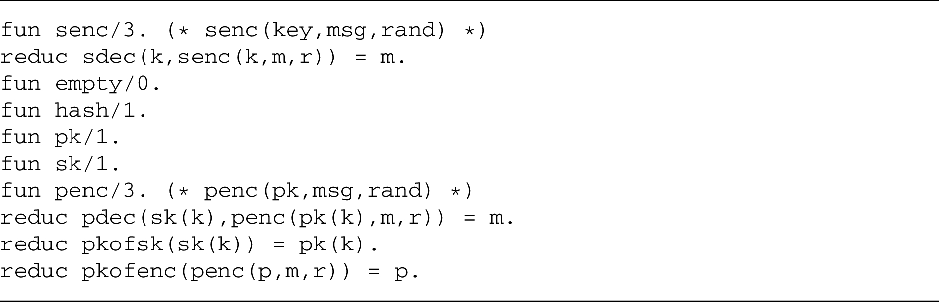
We first define the symbolic model used in this section. The constructors are: $penc / 3$ , $pk / 1$ , $sk / 1$ , $senc / 3$ , $(\cdot, \cdot)$ , $hash / 1$ , and $empty / 0$ , representing public-key encryption, public and secret keys, symmetric encryption, pairs, hashing, and empty messages, respectively. Encryption has a third argument modeling randomness used for encrypting. More specifically, $penc (pk (k), m, r)$ models a public key encryption using key $pk (k)$ , plaintext m, and randomness r, and $senc (k, m, r)$ a symmetric encryption using key k, plaintext m, and randomness r. We believe that $senc$ without the additional randomness argument r would also work in our setting. However, we introduce this additional nonce to help Proverif, which can then better distinguish ciphertexts (e.g., one of the Proverif scripts in the proof of Lemma 8.6 (Fig. 8 in the Online supplement) fails without r due to Proverif’s overapproximation technique). We have no equations in our theory.

Furthermore we have the destructors $pdec / 2$ , $sdec / 2$ , $pkofsk / 1$ , and $pkofenc / 1$ , modeling public-key decryption, symmetric decryption, extraction of a public key from a secret key, and extraction of a public key from a ciphertext. (The latter two are not needed in our protocols, but we provide them to make the adversary more realistic.) The behavior of the destructors is specified by the following rewrite rules: $\begin{array}{rcl} pdec (sk (x), penc (pk (x), y, z)) \to y \\ sdec (x, senc (x, y, z)) \to y \\ pkofsk (sk (x)) \to pk (x) \\ pkofenc (penc (x, y, z)) \to x \end{array}$ The Proverif code for this symbolic model is given in Fig. 3.

Fig. 3.

Key-exchange example: Proverif code for the symbolic model (secchan-model.pv, see Proverif input files in the Online supplement).

8.1. Key exchange using NSL

With the symbolic model set up we next show how to tailor a UC-secure key exchange from $NSL$ using a PKI functionality $F_{PKI}$ . Towards this goal we model the ideal key exchange functionality $F_{KE}$ , the PKI $F_{PKI}$ and the $NSL$ protocol based on $F_{PKI}$ as follows:

Definition 8.1 (Key exchange functionality).

$\begin{matrix} F_{KE} : = ν k . ({net}_{delA} () . \overline{{io}_{ka}} ⟨ k ⟩ ∣ {net}_{delB} () . \overline{{io}_{kb}} ⟨ k ⟩) \end{matrix}$

Definition 8.2 (Public key infrastructure functionality).

$\begin{array}{rcl} F_{PKI} : = ν k_{a} k_{b} . (\overline{{io}_{pkeA}} ⟨ (sk (k_{a}), pk (k_{a}), pk (k_{b})) ⟩ \\ ∣ \overline{{io}_{pkeB}} ⟨ (sk (k_{b}), pk (k_{a}), pk (k_{b})) ⟩ \\ ∣ \overline{{net}_{pke}} ⟨ (pk (k_{a}), pk (k_{b})) ⟩) \end{array}$

Definition 8.3 (Needham–Schroeder–Lowe).

$\begin{array}{rcl} {NSL}_{A} : = {io}_{pkeA} ((x_{sk},_, x_{{pk}_{B}})) . (ν n_{a}, A) . ν r_{1} . \\ \overline{{net}_{nslA}} ⟨ penc (x_{{pk}_{B}}, n_{a}, r_{1}) ⟩ . {net}_{nslA} (x_{c}) . \\ let (= n_{a}, x_{n_{b}}, = B) = pdec (x_{sk}, x_{c}) in \\ ν r_{2} . \overline{{net}_{nslA}} ⟨ penc (x_{{pk}_{B}}, x_{n_{b}}, r_{2}) ⟩ . \\ \overline{{io}_{ka}} ⟨ hash ((n_{a}, x_{n_{b}})) ⟩ \\ {NSL}_{B} : = {io}_{pkeB} ((x_{sk}, x_{{pk}_{A}},_)) . {net}_{nslB} (x_{c}) . \\ let (x_{n_{a}}, = A) = pdec (x_{sk}, x_{c}) in \\ ν n_{b} . ν r . \overline{{net}_{nslB}} ⟨ penc (x_{{pk}_{A}}, (x_{n_{a}}, n_{b}, B), r) ⟩ . \\ {net}_{nslB} (x_{c}^{'}) . if n_{b} = pdec (x_{sk}, x_{c}^{'}) then \\ \overline{{io}_{kb}} ⟨ hash ((x_{n_{a}}, n_{b})) ⟩ \\ NSL : = ν {io}_{pkeA} {io}_{pkeB} . ({NSL}_{A} ∣ {NSL}_{B} ∣ F_{PKI}) \end{array}$

The differences to the original NSL protocol [25] are: The original protocol does not specify what to do with the nonces $n_{a}$ , $n_{b}$ , while we use them to derive a key $hash ((n_{a}, n_{b}))$ . Also, [25] also presents an extended version of the protocol that explicitly communicates with a server S for getting the keys for Alice and Bob. We could get this extended protocol by proving that this retrieval protocol implements $F_{PKI}$ , and then composing our NSL protocol with the retrieval protocol.

We can now state the first result of this section, namely that the $NSL$ is a UC-secure realization of $F_{KE}$ .

Lemma 8.4.
$NSL ⩽ F_{KE}$ .

The proof of this lemma is given in the Supplemental material (Section I.1). We only show the simulator $(S, φ, \underline{n})$ here: $S : = ν k_{a} k_{b} . ({NSL}_{A}^{″} | {NSL}_{B}^{″} | \overline{{net}_{pke}} ⟨ (pk (k_{a}), pk (k_{b})) ⟩)$ , φ the identity, $\underline{n} : = {net}_{delA} {net}_{delB}$ where ${NSL}_{A}^{'}$ is ${NSL}_{A}$ without the initial ${io}_{pkeA} ((x_{sk},_, x_{{pk}_{B}}))$ , ${NSL}_{B}^{'}$ analogously, ${NSL}_{A}^{″} : = {NSL}_{A}^{'} {{net}_{delA} / {io}_{ka}, sk (k_{a}) / x_{sk}, pk (k_{b}) / x_{{pk}_{B}}}$ and ${NSL}_{B}^{″} : = {NSL}_{B}^{'} {{net}_{delB} / {io}_{kb}, sk (k_{b}) / x_{sk}, pk (k_{a}) / x_{{pk}_{A}}}$ .
8.2. Secure channel from key exchange

Next, we realize a secure channel. Since we already have a realization of a secure key exchange at hand, we realize the secure channel $SC$ from the idealized key exchange $F_{KE}$ . Later we replace $F_{KE}$ by $NSL$ .

Definition 8.5 (Secure channel protocol).

$\begin{array}{rcl} {SC}_{A} : = {io}_{ka} (x_{k}) . {io}_{A} (x_{m}) . ν r . \overline{{net}_{A}} ⟨ senc (x_{k}, x_{m}, r) ⟩ \\ {SC}_{B} : = {io}_{kb} (x_{k}) . {net}_{B} (x_{c}) . let x_{m} = sdec (x_{k}, x_{c}) in \overline{{io}_{B}} ⟨ x_{m} ⟩ \\ SC : = ν {io}_{ka} {io}_{kb} . ({SC}_{A} | {SC}_{B} | F_{KE}) \end{array}$

Lemma 8.6.
$SC ⩽ F_{SC}$ . ( $F_{SC}$ was defined in Definition 6.2 . )

The proof of this lemma is given in the Supplemental material (Section I.2). We only show the simulator $(S, φ, \underline{n})$ here: $\begin{array}{rcl} S & : = & ν k r . ({net}_{delB} () . {net}_{B} (x_{c}) . \\ let x_{m} = sdec (k, x_{c}) in \overline{{net}_{deliver}} ⟨ ⟩ \\ ∣ {net}_{notify} () . \overline{{net}_{A}} ⟨ senc (k, empty, r) ⟩), \end{array}$ $φ : = {{net}_{delA} / {net}_{scstart}}$ and $\underline{n} : = {net}_{deliver} {net}_{notify}$ .

With $NSL ⩽ F_{KE}$ (Lemma 8.4) and $SC ⩽ F_{SC}$ (Lemma 8.6) at hand we can now use the compositional capabilities of UC: We define an evaluation context $C [□] : = ν {io}_{ka} {io}_{kb} . ({SC}_{A} | {SC}_{B} | □)$ where ${SC}_{A}$ and ${SC}_{B}$ are the processes from Definition 8.5. Since $C$ meets the requirements of Theorem 5.10 $NSL ⩽ F_{KE}$ implies $C [NSL] ⩽ C [F_{KE}]$ . Since $C [F_{KE}] = SC$ and $SC ⩽ F_{SC}$ we have, by transitivity of ⩽ (Lemma 4.5), $C [NSL] ⩽ F_{SC}$ .

We did construct a secure channel from a PKI using the NSL protocol. More interesting than this result is the way we achieved it: We did not have to analyze the complete system $C [NSL]$ in one piece but could replace the $NSL$ protocol with an idealized functionality. This illustrates two striking advantages of the UC approach:
The fact that $NSL$ realizes an ideal key exchange can be re-used for security proofs of further systems.

We cannot only plug $NSL$ into $C$ but any protocol that realizes a secure key exchange (e.g., if no PKI is available and thus $NSL$ is not an option).
Instead of one monolithic security proof for $C [NSL]$ we end up with smaller proofs and results which can be used flexibly. Furthermore, to split the security analysis of a complex system into smaller parts might be the only feasible option to tackle it at all.
8.3. Generating many keys from one

While the example until now illustrates composition and the power of UC, $C [NSL]$ only realizes a single-use secure channel. To transfer multiple messages, we could just use concurrent composition to have $!! C [NSL] ⩽!! F_{SC}$ . However, the resulting protocol uses one instance of $NSL$ per message, and – since $NSL$ contains $F_{PKI}$ , another PKI for each message that is sent. This is clearly unrealistic. To get rid of this overhead we want to have all the instances of $SC$ to jointly use just one key exchange $F_{KE}$ , i.e., we want to use the previously mentioned joined state technique here. Towards this goal we model a wrapper protocol ${KE}^{*}$ which uses one key exchange to emulate multiple key exchanges (from a key k it derives session keys $hash ((sid, k))$ where $sid$ is the session id). Formally, we define ${KE}^{*}$ as follows and then show ${KE}^{*} ⩽!! F_{KE}$ .

Definition 8.7.
$\begin{array}{rcl} {KE}_{A}^{} : = {io}_{ka}^{'} (x_{k}) .!!_{x_{sid}} \overline{{io}_{ka}} ⟨ hash ((x_{sid}, x_{k})) ⟩ \\ {KE}_{B}^{} : = {io}_{kb}^{'} (x_{k}) .!!_{x_{sid}} \overline{{io}_{kb}} ⟨ hash ((x_{sid}, x_{k})) ⟩ \\ {KE}^{} : = ν {io}_{ka}^{'} {io}_{kb}^{'} . ({KE}_{A}^{} ∣ {KE}_{B}^{} ∣ F_{KE}^{'}) \end{array}$

where $F_{KE}^{'} : = F_{KE} {{io}_{ka}^{'} / {io}_{ka}, {io}_{kb}^{'} / {io}_{kb}}$ .
Lemma 8.8.
${KE}^{} ⩽!! F_{KE}$ .

The proof of this lemma is given in the Supplemental material (Section I.3). We only show the simulator $(S, φ, \underline{n})$ here: $S : = {net}_{delA} () .!! \overline{{net}_{delA}^{'}} ⟨ ⟩ ∣ {net}_{delB} () .!! \overline{{net}_{delB}^{'}} ⟨ ⟩$ , $φ : = {{net}_{delA}^{'} / {net}_{delA}, {net}_{delB}^{'} / {net}_{delB}}$ and $\underline{n} : = {net}_{delA}^{'} {net}_{delB}^{'}$ . This proof is the only one in this paper in which we could not outsource all proofs that actually involve the details of the cryptographic primitives to Proverif. This is because Proverif cannot understand $!!_{x}$ , and the lemma relies on the fact that $!!_{x}$ ensures that no two processes with the same session id are created.

Analogously to the single session case we define a suitable context $C^{}$ by replacing $F_{KE}^{'}$ in ${KE}^{}$ with □ and have $\begin{matrix} C^{} [NSL] ⩽ C^{} [F_{KE}^{'}] = {KE}^{} ⩽!! F_{KE} \end{matrix}$

Furthermore, $!! SC \approx ν {io}_{ka} {io}_{kb} . (!! {SC}_{A} |!! {SC}_{B} |!! F_{KE})$ (by Lemmas 5.8, 5.9). Hence $\begin{array}{rcl} ν {io}_{ka} {io}_{kb} . (!! {SC}_{A} |!! {SC}_{B} | C^{} [NSL]) \\ ⩽ ν {io}_{ka} {io}_{kb} . (!! {SC}_{A} |!! {SC}_{B} |!! F_{KE}) \\ ⩽!! SC ⩽!! F_{SC} . \end{array}$

Finally, we have a protocol which realizes multiple secure channels while invoking the $NSL$ protocol and using only one PKI.
9. Virtual primitives

In this section, we present a technique for deriving security of protocols in the symbolic UC model that is specific to the symbolic model. No analogue in the computational world seems to exist. The idea is the following: When constructing UC secure protocols, it is often necessary to include specific “trapdoors” that allow the simulator to extract or modify certain information. For example, when constructing a simulator for a commitment scheme, we need to include in the protocol some way for the simulator to extract the value of the commitment when given a commitment by the environment (extractability), or to change the content of a commitment when producing a commitment for the environment (equivocality), see [13]. These additional trapdoors often make the protocols more complex, and they often also need more complex cryptographic primitives. A simple commitment protocol in which the committer just sends $hash (m, r)$ for message m and randomness r is not UC secure because the simulator cannot extract or equivoke. Instead, one would need to assume a special hash function that takes an additional parameter $crs$ (the common reference string) $hash (crs, m, r)$ in such a way that given a suitably chosen “fake” $crs$ , one can find collisions in $hash$ or extract m from $hash (crs, m, r)$ . With such a hash function, one can construct a UC secure commitment relatively easily (see Definition 9.3 below). However, now our protocol uses a considerably more complex primitive than a simple hash function. And certainly common hash functions such as SHA-3 do not have these properties.

This leads to a strange situation: We have a protocol that we can only prove secure using a hash function that has additional weaknesses (namely that given a “bad” crs, one can cheat). One might be tempted to state that if the protocol is secure for such weak hash functions, it should in particular be secure for good hash functions. Unfortunately, such reasoning does not work in the computational setting: We cannot just remove the existence of trapdoors from the hash function – if we do so, we have a completely different hash function and our security proof makes no claims about that function.

In the symbolic world, things are different. Here it turns out that we can indeed first analyze a protocol using a hash function with trapdoors, and then remove these trapdoors in a later step, still preserving security. We call this approach the “virtual primitives” approach, because we use primitives (in this example a hash function with trapdoors) that do not need to actually exist, and that are removed in the final protocol.

In a nutshell, the virtual primitives approach when trying to realize a functionality $F$ (e.g., a commitment) works as follows:

First, identify a symbolic model $M_{real}$ containing cryptographic primitives (e.g. a hash function) that should be used in the final protocol.

Extend $M_{real}$ by additional constructors, destructors, or equality rules, call the resulting model $M_{virt}$ . The extension $M_{virt}$ should be “safe” in the sense that in $M_{virt}$ an adversary will have at least as much power as in $M_{real}$ (this will be made formal in Section 9.2).

Design a protocol P. Show that P emulates $F$ with respect to $M_{virt}$ .

Compose P with other protocols, leading to a complex protocol $C [P] ⩽ C [F] ⩽ G$ (with respect to $M_{virt}$ ) where $G$ is some desired final goal, e.g., some crypto-heavy voting protocol.

Property preservation guarantees that any property ℘ that holds for $G$ also holds for $C [P]$ (with respect to $M_{virt}$ ). Since $M_{virt}$ only makes adversaries stronger, ℘ also holds for $C [P]$ with respect to $M_{real}$ .

Summarizing, we have constructed a protocol $C [P]$ in a modular way such that $C [P]$ uses the symbolic model $M_{real}$ (without any trapdoors) and has all the security properties of the functionality $G$ .

The virtual primitive approach is not limited to commitments. But in the following sections, we illustrate it in the case of a commitment protocol. Note however, that the main theorem that allows us to conclude that $M_{virt}$ -security implies $M_{real}$ -security is formulated for general safe extensions.

A few words are in order why the virtual primitives approach works in the symbolic setting. What is the specific property of the symbolic model – in contrast to the computational one – that makes it possible? In our interpretation, this is due to the fact that a primitive (like hashes) in the symbolic world is a concrete object (i.e., a particular constructor with certain reduction rules and equalities) while in the computational world it is a class of objects (hash functions) that are described by some negative properties (“functions such that the adversary cannot…”). Therefore in the symbolic world, it is possible to formally compare executions using different kinds of a primitive (e.g., hashes with and without trapdoors); executions in one setting can be mapped into executions in the other setting by rewriting the terms sent around. In contrast, in the computational setting, this is not possible: a security result for hash functions with trapdoors has no implications for hash functions without trapdoors – these two are completely different mathematical functions on bitstrings, and it is not possible to rewrite an execution that uses one hash function into an execution using another (in particular if the adversary makes his actions depend on individual bits of the hashes). This difference between the symbolic and the computational setting seems to be the reason why virtual primitives work in the symbolic setting.

Related approaches in the computational model. Although virtual primitives as described above are restricted to the symbolic setting, somewhat related techniques do exist in the computational model. [4,27] show how to circumvent UC impossibility results (such as the impossibility of oblivious transfer, commitment, or general multi-party computation without trusted setup) by giving the simulator additional power. Namely the simulator is allowed to run in (slightly) superpolynomial time. This is in some sense similar to giving the simulator access to additional constructors/destructors for extraction/equivocation as we do. Yet, there are three crucial differences to our setting: First, they can only use primitives that can actually exist computationally. For example, even a superpolynomial-time simulator cannot invert a fixed-length hash function, as part of the input is information-theoretically lost. In contrast, we can add arbitrary properties to, e.g., hash functions by introducing new equations in the symbolic model. Second, their final protocols have to use whatever primitives have been introduced for proof purposes; it is not possible to remove additional properties in the end as done in our approach. Third, their protocols involve advanced cryptographic techniques which makes the protocols considerably more involved and, consequently, inefficient. On the other hand, of course, protocols designed with our techniques are only proven secure in the symbolic model but lack a proof in the computational model – we believe therefore that our and their approaches are incomparable with respect to their advantages and disadvantages.

9.1. Realizing commitments

For simplicity, we formulate a commitment functionality where the adversary is not informed that a commitment takes place (when both Alice and Bob are honest). Of course, such a functionality can only be realized if we assume perfectly secure channels between Alice and Bob that do not even allow the adversary to notice or block messages. If our protocols were to use secure channels where the adversary can notice and block communication, we would instead realize a somewhat weaker functionality which notifies the adversary12

¹²
Namely, $F_{COM} : = {io}_{coma} (x_{m}) . (\overline{{net}_{coma}} ⟨ ⟩ | {net}_{comb} () . \overline{{io}_{comb}} ⟨ ⟩ | {io}_{opena} () . (\overline{{net}_{opena}} ⟨ ⟩ | {net}_{openb} () . \overline{{io}_{openb}} ⟨ x_{m} ⟩))$ .

(the resulting changes in the proof are orthogonal to the issues of this chapter).

Definition 9.1 (Commitment).

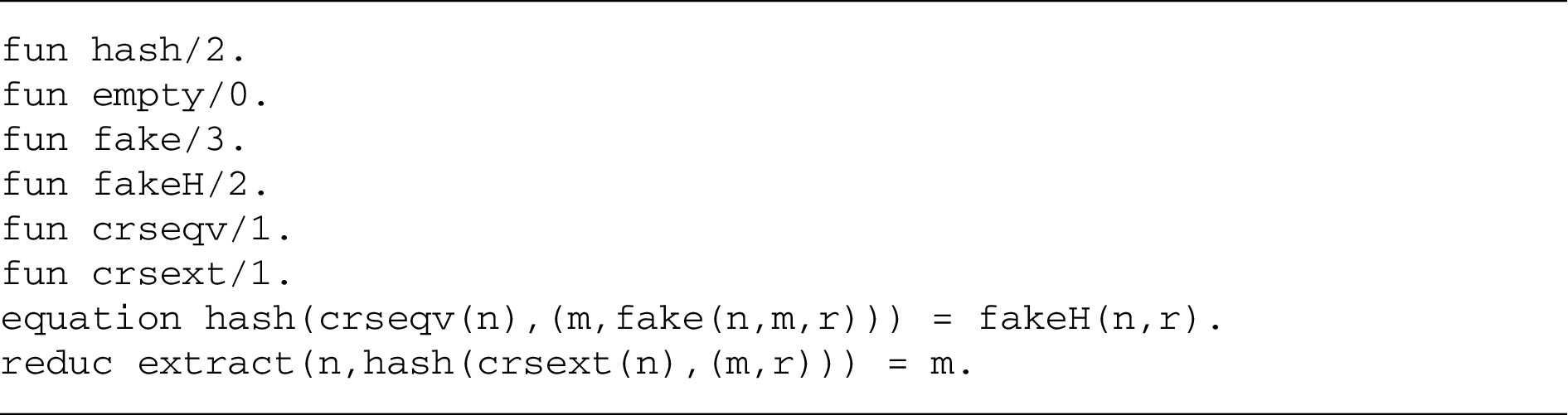
$F_{COM} : = {io}_{coma} (x_{m}) . (\overline{{io}_{comb}} ⟨ ⟩ | {io}_{opena} () . \overline{{io}_{openb}} ⟨ x_{m} ⟩)$ .

Symbolic model. The symbolic model $M_{real}$ has constructors $hash / 2$ , $empty / 0$ , and $(\cdot, \cdot)$ (pairs) – $f / n$ means f has arity n –, has destructors $fst$ , $snd$ , has no equalities, and has the rewrite rules for $fst$ , $snd$ , $equals$ prescribed by Definition 2.1. This model $M_{real}$ is quite standard and does not use any cryptography except hash functions ( $hash$ is binary for convenience only).

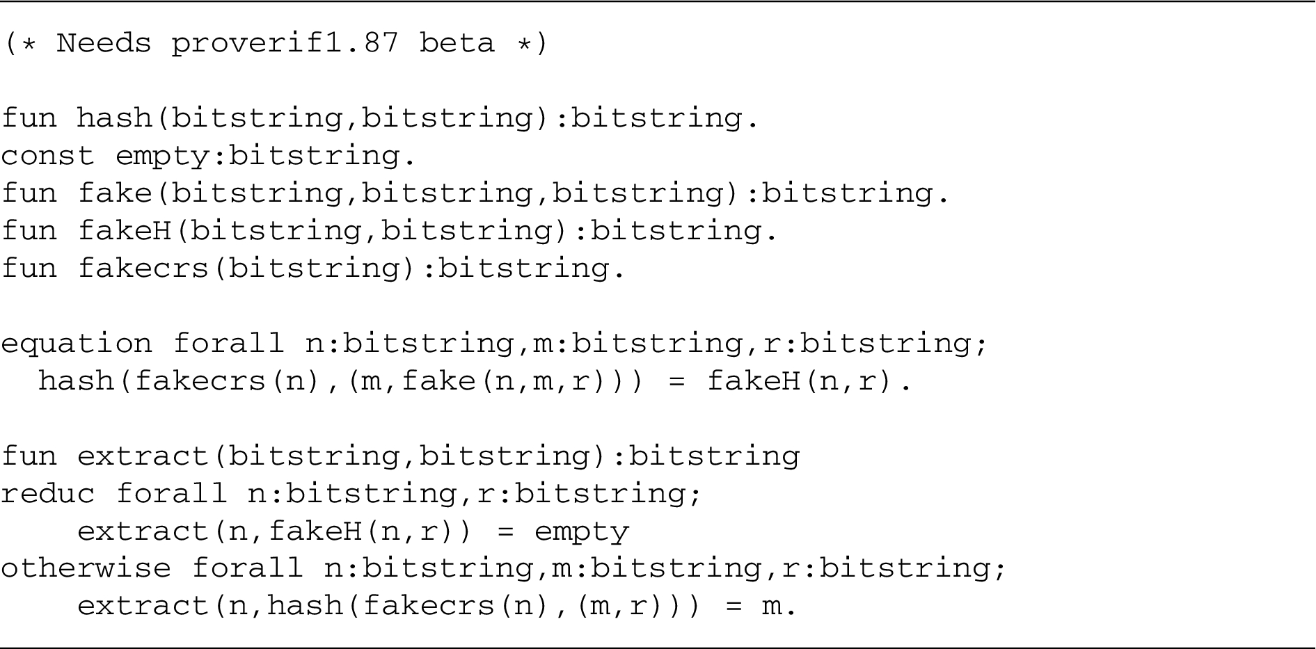
As explained above, to construct UC-secure commitments, we need additional “trapdoors” in our equational theory. Let $M_{virt}$ be the symbolic model $M_{real}$ with the following additions: Constructors $fake / 3$ , $fakeH / 2$ , $crseqv / 1$ , $crsext / 1$ , destructor $extract / 2$ , equation $hash (crseqv (x_{n}), (x_{m}, fake (x_{n}, x_{m}, x_{r}))) =_{E} fakeH (x_{n}, x_{r})$ , and rewrite rule $extract (x_{n}, hash (crsext (x_{n}), (x_{m}, x_{r}))) \to x_{m}$ .

The Proverif code for this symbolic model is given in Fig. 4.

Fig. 4.

Virtual primitives example: Proverif code for the symbolic model (virtprim-model.pv, see Proverif input files in the Online supplement).

Notice that if we have a CRS $crseqv (n)$ and know n, we can open $fakeH (n, r)$ to arbitrary values. Similarly, if the CRS is $crsext (n)$ and we know n, we can extract m from $hash (crsext (n), (m, r))$ . These two facts allow us to construct a simulator that does equivocation and extraction.

Note that we introduced two different CRS-constructors for faking, $crsext$ and $crseqv$ . It would be tempting to use only one of them, i.e., use the equation $hash (fakecrs (x), (y, fake (x, y, z))) =_{E} fakeH (x, z)$ and the reduction rule $extract (x, hash (fakecrs (x), (y, z))) \to y$ . But then we would have for any terms k, m, r that $extract (k, fakeH (k, r)) =_{E} extract (k, hash (fakecrs (k), (m, r))) \to m$ , so by computing $extract (k, fake (k, r))$ the adversary can derive any term m, thus the adversary will know all secrets. This is clearly not a sensible symbolic model.

The commitment protocol. The protocol we construct uses a crs, so we first need to define the crs functionality $F_{CRS}$ that gives a random non-secret value k to Alice, Bob, and the adversary.

Definition 9.2 (Common reference string).

$F_{CRS} : = ν k . (\overline{{io}_{crsa}} ⟨ k ⟩ ∣ \overline{{io}_{crsb}} ⟨ k ⟩ ∣ \overline{{net}_{crs}} ⟨ k ⟩)$ .

Our protocol is then as expected. To commit to a message $x_{m}$ , Alice fetches the crs $x_{crs}$ , picks a random r, and sends $h : = hash (x_{crs}, (x_{m}, r))$ to Bob. To unveil, Alice sends $(x_{m}, r)$ , so that Bob can check whether h indeed contained these values. We call Alice’s part of the protocol ${COM}_{A}$ and Bob’s part ${COM}_{B}$ .

Definition 9.3 (Commitment protocol).

$\begin{array}{rcl} {COM}_{A} : = {io}_{crsa} (x_{crs}) . {io}_{coma} (x_{m}) . \\ ν r . (\overline{{net}_{1}} ⟨ hash (x_{crs}, (x_{m}, r)) ⟩ | {io}_{opena} () . \overline{{net}_{2}} ⟨ (x_{m}, r) ⟩) \\ {COM}_{B} : = {io}_{crsb} (x_{crs}) . {net}_{1} (x_{h}) . (\overline{{io}_{comb}} ⟨ ⟩ | {net}_{2} ((x_{m}, x_{r})) . \\ if x_{h} = hash (x_{crs}, (x_{m}, x_{r})) then \overline{{io}_{openb}} ⟨ x_{m} ⟩) \\ COM : = ν {io}_{crsa} {io}_{crsb} {net}_{1} {net}_{2} . ({COM}_{A} | {COM}_{B} | F_{CRS}) \end{array}$

To show that $COM$ is a secure commitment protocol, we need to show the following lemma (cf. also the discussion on how to model corruptions in Section 4).

Lemma 9.4.
With respect to $M_{virt}$ , we have
Uncorrupted case: $COM ⩽ F_{COM}$ .

Alice corrupted: $ν {io}_{crsb} . ({COM}_{B} | F_{CRS} {\frac{{net}_{crsa}}{{io}_{crsa}}}) ⩽ F_{COM} {\frac{{net}_{coma}}{{io}_{coma}}, \frac{{net}_{opena}}{{io}_{opena}}}$ .

Bob corrupted: $ν {io}_{crsa} . ({COM}_{A} | F_{CRS} {\frac{{net}_{crsb}}{{io}_{crsb}}}) ⩽ F_{COM} {\frac{{net}_{comb}}{{io}_{comb}}, \frac{{net}_{openb}}{{io}_{openb}}}$ .

The proof of this lemma is given in the Supplemental material (Section J.1), we only show the simulators $(S, φ, \underline{n})$ for the three cases here:

Uncorrupted case: $S = ν k r . \overline{{net}_{crs}} ⟨ k ⟩$ . φ the identity. $\underline{n} = \emptyset$ .

Alice corrupted: $\begin{array}{rcl} S & : = & ν k . (\overline{{net}_{crsa}} ⟨ crsext (k) ⟩ ∣ \overline{{net}_{crs}} ⟨ crsext (k) ⟩ ∣ {net}_{1} (x_{h}) . \\ (\overline{{net}_{coma}} ⟨ extract (k, x_{h}) ⟩ ∣ {net}_{2} ((x_{m}, x_{r})) . \\ if x_{h} = hash (crsext (k), (x_{m}, x_{r})) then \overline{{net}_{opena}} ⟨ ⟩)) \end{array}$ φ the identity. $\underline{n} = {net}_{coma} {net}_{opena}$ .

Bob corrupted: $\begin{array}{rcl} S & : = & ν k r . (\overline{{net}_{crsb}} ⟨ crseqv (k) ⟩ ∣ \overline{{net}_{crs}} ⟨ crseqv (k) ⟩ \\ ∣ {net}_{comb} () . (\overline{{net}_{1}} ⟨ fakeH (k, r) ⟩ \\ ∣ {net}_{openb} (x_{m}^{'}) . \overline{{net}_{2}} ⟨ (x_{m}^{'}, fake (k, x_{m}^{'}, r)) ⟩)) \end{array}$ φ the identity. $\underline{n} = {net}_{comb} {net}_{openb}$ .

We show the corresponding observational equivalences by a sequence of rewriting steps on the protocol, interspersed with automated Proverif proofs for the steps that actually involve the symbolic model (i.e., we do not have to manually deal with the complex symbolic model $M_{virt}$ ).
9.1.1. A note on adaptive corruption

We have only modeled static corruption in our examples, i.e., it is fixed in the beginning of the execution which parties are corrupted. If we were to model adaptive corruption where parties may be corrupted during the protocol execution, we would face an additional challenge (besides the fact that the descriptions of the processes would be much more complex): Since the simulator may have to provide the CRS before he knows whether Alice or Bob will be corrupted, he will not know whether he should use $crseqv (k)$ or $crsext (k)$ as CRS. And on p. 27 we explained why we cannot just replace both $crseqv$ and $crseqv$ by a single constructor $fakecrs$ because then the adversary would be able to deduce any term. However, this problem can be solved using the conditional destructors supported by Proverif 1.87: we can make sure that the rewrite rule $extract (x_{n}, hash (crsext (x_{n}), (x_{m}, x_{r}))) \to x_{m}$ only triggers if $hash (crsext (x_{n}), (x_{m}, x_{r})) \neq_{E} fakeH (M, M^{'})$ for all M, $M^{'}$ . The resulting symbolic model is shown in Fig. 5. We can show Lemma 9.4 also using this symbolic model by replacing all occurrences of $crseqv$ and $crsext$ in the simulators by $fakecrs$ . Proverif still shows all the necessary equivalences. Although this does not show adaptive security, it shows that the simulator does not need to choose the CRS depending on who is corrupted, giving hope for the adaptive case. We leave that case for future work.

9.2. Removing the virtual primitives

In this section, we will consider different symbolic models. Since the relation symbols →, ⇓, ≈, $↓_{}$ , $=_{E}$ etc. do not explicitly specify the symbolic model, we use the following convention: When referring to a symbolic model $M_{i}$ , we write $\to_{i}$ , $⇓_{i}$ , $\approx_{i}$ , $↓_{}^{i}$ , $=_{E_{i}}$ etc. We say a term (or destructor term) is an $M$ -term (or $M$ -destructor term) if it contains only constructors (and destructors) from $M$ . We call a process an $M$ -process if it contains only $M$ -terms and $M$ -destructor terms.

We have now shown that $COM$ is a secure commitment protocol with respect to $M_{virt}$ . However, we would like to deduce security of protocols using $COM$ with respect to $M_{real}$ . For this, we first need to formalize what it means that $M_{virt}$ is a safe extension of $M_{real}$ in the following definition.

Definition 9.5 (Safe extension).

We call a symbolic model $M_{1} = (Σ_{1}, E_{1}, R_{1})$ a safe extension of a symbolic model $M_{2} = (Σ_{2}, E_{2}, R_{2})$ iff the following holds:

$Σ_{1} \supseteq Σ_{2}$ .

If D is an $M_{2}$ -destructor term, and M is an $M_{1}$ -term, and $D ⇓_{1} M$ , then there exists an $M_{2}$ -term $M^{'} =_{E_{1}} M$ with $D ⇓_{2} M^{'}$ .

For all $M_{2}$ -destructor terms D and $M_{2}$ -terms M, we have $D ⇓_{2} M \Rightarrow D ⇓_{1} M$ .

For all $M_{2}$ -terms M, $M^{'}$ we have $M =_{E_{1}} M^{'} \Leftrightarrow M =_{E_{2}} M^{'}$ .

The following lemma is relatively easy to show.

Lemma 9.6.
$M_{virt}$ is a safe extension of $M_{real}$ .

The following theorem justifies the above definition of safe extensions.
Theorem 9.7.
Assume that $M_{1}$ is a safe extension of $M_{2}$ . Then $M_{2}$ -terms M, we have P, $P^{'}$ , we have for all $M_{2}$ -processes P, $P^{'}$ we have $P \approx_{1} P^{'} \Rightarrow P \approx_{2} P^{'}$ .

Fig. 5.
Virtual primitives example: Proverif code for the symbolic model when using $fakecrs$ constructor (virtprim-model-x.pv, see Proverif input files in the Online supplement). Note that we use the typed Proverif syntax here because Proverif 1.87 does not support conditional destructors in the untyped syntax.

Now we can finally state the following result that derives security of $COM$ with respect to $M_{real}$ in any context (we state it generally, though).
Lemma 9.8.
Let P, $F$ be $M_{real}$ -processes (representing a protocol and an ideal functionality, e.g., $P = COM$ and $F = F_{COM}$ ). Let $M_{virt}$ be a safe extension of $M_{real}$ . Assume that $P ⩽_{virt} F$ .

Let C be an $M_{real}$ -context whose hole is protected only by $ν io$ for IO-names $io$ , by parallel compositions, and by !, and that does not contain any NET-names in $fn (P, F)$ . Assume that $C [F] ⩽_{virt} G$ for some $M_{real}$ -process $G$ .

Let $E_{1}$ , $E_{2}$ be $M_{real}$ -contexts satisfying the conditions of Theorem 6.1 (property preservation).

If $E_{1} [G] \approx_{virt} E_{2} [G]$ then $E_{1} [C [P]] \approx_{real} E_{2} [C [P]]$ .
Proof.
By the composition theorem (Theorem 5.10), $P ⩽_{virt} F$ implies $C [P] ⩽_{virt} C [F]$ . With transitivity and $C [F] ⩽_{virt} G$ , this implies $C [P] ⩽_{virt} G$ . Then by the property preservation theorem (Theorem 6.1), $E_{1} [G] \approx_{virt} E_{2} [G]$ implies $E_{1} [C [P]] \approx_{virt} E_{2} [C [P]]$ . Since $M_{virt}$ is a safe extension of $M_{real}$ , this implies $E_{1} [C [P]] \approx_{real} E_{2} [C [P]]$ by Theorem 9.7. □
9.3. On removing the CRS

Using virtual primitives, we have managed to get rid of the need for trapdoors in our commitment protocol. However, we still use a common reference string. This leads to the question whether the CRS can also be removed from the protocol. We do not answer that question here, but we give some indications as to how it might be possible to remove the CRS, also.

First, the question is whether we can construct a UC secure commitment protocol without using a CRS in the first place (i.e., instead of the protocol from Section 9.1). We know that this is impossible in the computational UC setting (no matter what primitives we use) [13]. Unfortunately, their impossibility result carries over to the symbolic setting in the following lemma.

Lemma 9.9.

There are no closed processes A, B and NET-names $\underline{net}$ with the following three properties:

$ν \underline{net} . (A | B) ⩽ F_{COM}$ .(Uncorrupted case.)

$A ⩽ F_{COM} {\frac{{net}_{comb}}{{io}_{comb}}, \frac{{net}_{openb}}{{io}_{openb}}}$ .(Bob corrupted.)

$B ⩽ F_{COM} {\frac{{net}_{coma}}{{io}_{coma}}, \frac{{net}_{opena}}{{io}_{opena}}}$ .(Alice corrupted.)

Thus, a UC secure commitment protocol has to be of the form $ν \underline{net} . (A | B | F)$ for some functionality $F$ , e.g., $F_{CRS}$ .

Proof of Lemma 9.9.

Assume that there are such processes A, B and NET-names $\underline{net}$ .

Then there are simulators $(S_{0}, φ_{0}, {\underline{n}}_{0})$ , $(S_{A}, φ_{A}, {\underline{n}}_{A})$ , and $(S_{B}, φ_{B}, {\underline{n}}_{B})$ such that $\begin{array}{rcl} (1) & ν \underline{net} . (A | B) \approx ν {\underline{n}}_{0} . (F_{COM} φ_{0} | S_{0}) = ν {\underline{n}}_{0} . (F_{COM} | S_{0}) \\ (2) & A \approx ν {\underline{n}}_{A} . (F_{COM} {\frac{{net}_{comb}}{{io}_{comb}}, \frac{{net}_{openb}}{{io}_{openb}}} φ_{A} | S_{A}) = ν {\underline{n}}_{A} . (F_{COM} {\frac{{net}_{comb}^{'}}{{io}_{comb}}, \frac{{net}_{openb}^{'}}{{io}_{openb}}} | S_{A}) \\ (3) & B \approx ν {\underline{n}}_{B} . (F_{COM} {\frac{{net}_{coma}}{{io}_{coma}}, \frac{{net}_{opena}}{{io}_{opena}}} φ_{B} | S_{B}) = ν {\underline{n}}_{B} . (F_{COM} {\frac{{net}_{coma}^{'}}{{io}_{coma}}, \frac{{net}_{opena}^{'}}{{io}_{opena}}} | S_{B}) \end{array}$ for suitable names ${net}_{coma}^{'}$ , ${net}_{opena}^{'}$ , ${net}_{comb}^{'}$ , ${net}_{openb}^{'}$ . The equalities use the fact that $F_{COM}$ does not contain any NET-names.

Let $\begin{array}{rcl} E : = ν {io}_{coma} {io}_{comb} {io}_{opena} {io}_{openb} . \\ ((ν r . (\overline{{io}_{coma}} ⟨ r ⟩ | {io}_{comb} () . (\overline{{io}_{opena}} ⟨ ⟩ | {io}_{openb} (x) . if x = r then \overline{c} ⟨ ⟩))) | □) \end{array}$ where c is a fresh name. Intuitively, this context commits to a fresh nonce r, waits until the commit succeeds, then opens the commitment and checks whether the unveiled value is indeed r. For a “good” commitment scheme, this should always be the case. Indeed: By definition of $F_{COM}$ (and using that ${\underline{n}}_{0}$ does not contain IO-names), we have that $E [ν {\underline{n}}_{0} . (F_{COM} | S_{0})] \to^{*} ↓_{c}$ . By (1) we have $E [ν \underline{net} . (A | B)] \approx E [ν {\underline{n}}_{0} . (F_{COM} | S_{0})]$ and thus $E [ν \underline{net} . (A | B)] \to^{*} ↓_{c}$ .

We now use (2) and (3) to transform $E [ν \underline{net} . (A | B)]$ into a process that does not use the commitment protocol $A | B$ any more, but instead uses two instances of $F_{COM}$ : $\begin{array}{rcl} E [ν \underline{net} . (A | B)] \overset{(2, 3)}{\approx} E [ν \underline{net} . (ν {\underline{n}}_{A} . (F_{COM} {\frac{{net}_{comb}^{'}}{{io}_{comb}}, \frac{{net}_{openb}^{'}}{{io}_{openb}}} | S_{A}) \\ (4) & | ν {\underline{n}}_{B} . (F_{COM} {\frac{{net}_{coma}^{'}}{{io}_{coma}}, \frac{{net}_{opena}^{'}}{{io}_{opena}}} | S_{B}))] \end{array}$

We can show that the RHS of (4) never emits c. Intuitively, this is because E only emits c if it gets r back from the second $F_{COM}$ (via ${io}_{openb}$ ). However, r is only sent to the first $F_{COM}$ (via ${io}_{coma}$ ) and only revealed by the first $F_{COM}$ (due to a signal on ${io}_{opena}$ ) after the second $F_{COM}$ has gotten its value (which E can enforce by receiving on ${io}_{comb}$ ). Thus the value received from the second $F_{COM}$ cannot be r. To prove this formally, a lengthy calculation is required, we defer it to the Supplemental material (Section J.4). Since the RHS of (4) does not emit c but the LHS of (4) emits c, this contradicts the observational equivalence (4). Thus our assumption was wrong that processes A, B and NET-names $\underline{net}$ as in the statement of the lemma exist. □

However, Lemma 9.9 does not exclude that an approach similar to the virtual primitives approach might work: We first construct a UC secure commitment protocol (again, commitments are just one example), build a complex protocol from it using the composition theorem, and then show that security of the complex protocol implies (non-UC) security of a modification that does not use the CRS. It is likely that this works as the CRS returned by the CRS functionality is just a fresh public name, so instead of the CRS we should be able to just use some fresh (non-restricted) name a.

There is one subtlety, though: When composing the commitment protocol P, we end up with a complex protocol $C [P]$ that may use multiple instances of $F_{CRS}$ . In particular, if $C [P]$ contains $!! P$ , then $C [P]$ will contain an unbounded number of $F_{CRS}$ -instances. So we cannot replace $F_{CRS}$ just by a single name, we will need a way to generate an arbitrary number of fresh values. The obvious way for this is to use something like $hash (a, sid)$ instead of the CRS that we get from the $F_{CRS}$ -instance with session-id $sid$ (here a is a fresh name).

A lemma roughly like the following conjecture should therefore lead to a method for removing the CRS from a protocol that was produced by UC composition.

Conjecture 9.10.

Let $hash$ be a free constructor (i.e., not occurring in any equations or rewrite rules in the symbolic models). Let P be a process. Let $E_{1}$ , $E_{2}$ be contexts. Assume that $hash$ does not occur in $E_{1}$ , $E_{2}$ , P. Let $a \notin fn (E_{1}, E_{2}, P) \cup bn (E_{1}, E_{2}, P)$ .

Let $P^{'}$ result from P by replacing all subterms “ ${net}_{crsa} (x) . Q$ ” by “ $let x = a in Q$ ”. Then $E_{1} [ν {net}_{crsa} . (P | F_{CRS})] ≋ E_{2} [ν {net}_{crsa} . (P | F_{CRS})]$ implies $E_{1} [ν {net}_{crsa} . (P^{'})] ≋ E_{2} [ν {net}_{crsa} . (P^{'})]$ .

Let $P^{'}$ result from P by replacing all subterms “ $(M_{sid}, {net}_{crsa}) (x) . Q$ ” by “let $x = hash (a, M_{sid})$ in Q”. Then $E_{1} [ν {net}_{crsa} . (P |!! F_{CRS})] ≋ E_{2} [ν {net}_{crsa} . (P |!! F_{CRS})]$ implies $E_{1} [ν {net}_{crsa} . (P^{'})] ≋ E_{2} [ν {net}_{crsa} . (P^{'})]$ .

Proving (i) is probably considerably simpler than proving (ii). An alternative to proving (ii) could be to make sure that $C [P]$ does not contain $F_{CRS}$ under a $!!$ . This could be achieved if we design a commitment protocol P that does not implement $F_{COM}$ , but $!! F_{COM}$ (compare with Section 8.3). Then a single copy of P would be sufficient in $C [P]$ .

We leave further exploration of approaches to get rid of the CRS to future research.

Footnotes

Acknowledgments

We thank Stephanie Delaune for intensive discussions. Florian Böhl was supported by MWK grant “MoSeS”. Dominique Unruh was supported by the European Union through the European Regional Development Fund through the sub-measure “Supporting the development of R&D of info and communication technology”, by the European Social Fund’s Doctoral Studies and Internationalisation Programme DoRa, and by the Estonian Centre of Excellence in Computer Science, EXCS.

Limits for composition and property preservation

In this section, we show that the restrictions of the composition theorem are necessary. More precisely, we show that if $P ⩽ Q$ , then not necessarily $! P ⩽! Q$ or $io (x) . P ⩽ io (x) . Q$ or $\overline{io} ⟨ t ⟩ . P ⩽ \overline{io} ⟨ t ⟩ . Q$ or $ν net . P ⩽ ν net . Q$ or $P | R ⩽ Q | R$ (for R that has NET-names in common with P, Q). We show that this is not just a limitation of the composition theorem, we show that similar limitations also apply to property preservation. More precisely, property preservation $P ⩽ Q$ , $E_{1} [Q] \approx E_{2} [Q] \Rightarrow E_{1} [P] \approx E_{2} [P]$ does not necessarily hold if $E_{1}$ , $E_{2}$ contain a bang (!) over their hole, or an input/output over their hole, or an if/let over their hole, or a different number of $!!$ ’s over their respective holes, or restrict NET-names over their holes, or use NET-names.

The proofs of Lemmas A.5 and A.6 are identical to those of Lemmas A.3 and A.4, except that $io ()$ and $\overline{io} ⟨ empty ⟩$ are exchanged.

Remember that $if x = y$ is syntactic sugar for $let z = equals (x, y)$ . So this example is a counterexample for let-statements.

References

[1]

Arapinis,

Chothia,

Ritter and

Ryan, Analysing unlinkability and anonymity using the applied pi calculus, in: CSF 2010, 23rd IEEE Computer Security Foundations Symposium, IEEE, 2010, pp. 107–121.

[2]

Backes,

Pfitzmann and

Waidner, A composable cryptographic library with nested operations, in: Proceedings of the 10th ACM CCS, 2003, pp. 220–230.

[3]

Backes,

Pfitzmann and

Waidner, The reactive simulatability (RSIM) framework for asynchronous systems, Information and Computation 205(12) (2007), 1685–1720.

[4]

Barak and

Sahai, How to play almost any mental game over the net – Concurrent composition via super-polynomial simulation, in: Proceedings of the 46th IEEE Symposium on Foundations of Computer Science (FOCS), 2005, pp. 543–552.

[5]

Bengtson,

Bhargavan,

Fournet,

A.D.

Gordon and

Maffeis, Refinement types for secure implementations, ACM Transactions on Programming Languages and Systems (TOPLAS) 33 (2011), 8.

[6]

Blanchet, Automatic verification of correspondences for security protocols, Journal of Computer Security 17(4) (2009), 363–434.

[7]

Blanchet,

Abadi and

Fournet, Automated verification of selected equivalences for security protocols, Journal of Logic and Algebraic Programming 75 (2008), 3–51.

[8]

E.F.

Brickell,

Camenisch and

Chen, Direct anonymous attestation, in: Proceedings of the 11th ACM Conference on Computer and Communications Security, ACM Press, 2004, pp. 132–145.

[9]

Canetti, Universally composable security: A new paradigm for cryptographic protocols, in: Proceedings of the 42nd IEEE Symposium on Foundations of Computer Science (FOCS), 2001, pp. 136–145.

10.

[10]

Canetti,

Cheung,

Kaynar,

Liskov,

Lynch,

Pereira and

Segala, Task-structured probabilistic I/O automata, Technical Report MIT-CSAIL-TR-2006-060, MIT CSAIL, 2006, available at: http://dspace.mit.edu/handle/1721.1/33964.

11.

[11]

Canetti,

Cheung,

Kirli Kaynar,

Liskov,

N.A.

Lynch,

Pereira and

Segala, Time-bounded task-PIOAs: A framework for analyzing security protocols, in: DISC, 2006, pp. 238–253.

12.

[12]

Canetti,

Dodis,

Pass and

Walfish, Universally composable security with global setup, in: Proceedings of the 4th Theory of Cryptography Conference (TCC), 2007, pp. 61–85.

13.

[13]

Canetti and

Fischlin, Universally composable commitments, in: Advances in Cryptology, Proceedings of CRYPTO 2001,

Kilian, ed., LNCS, Vol. 2139, Springer, 2001, pp. 19–40, Full version available at: http://eprint.iacr.org/2001/055.ps.

14.

[14]

Canetti and

Herzog, Universally composable symbolic security analysis, Journal of Cryptology 24(1) (2011), 83–147.

15.

[15]

Canetti and

Rabin, Universal composition with joint state, in: Proceedings of CRYPTO 2003, LNCS, Vol. 2729, Springer, 2003, pp. 265–281.

16.

[16]

Canetti and

Vald, Universally composable security with local adversaries, in: SCN 2012,

Visconti and

De Prisco, eds, LNCS, Vol. 7485, Springer, 2012, pp. 281–301.

17.

[17] Cher , Bang bang (my baby shot me down). 7” single, 1966, Written by Sonny Bono, sound sample, available at: http://en.wikipedia.org/wiki/File:Cher-_Bang_Bang_My_Baby_Shot_Me_Down.ogg.

18.

[18]

Cheval and

Blanchet, Proving more observational equivalences with ProVerif, in: POST 2013,

Basin and

Mitchell, eds, LNCS, Vol. 7796, Springer, 2013, pp. 226–246.

19.

[19]

Datta,

Küsters,

J.C.

Mitchell and

Ramanathan, On the relationships between notions of simulation-based security, in: Theory of Cryptography, Proceedings of TCC 2005,

Kilian, ed., LNCS, Springer, 2005, pp. 476–494.

20.

[20]

Delaune,

Kremer and

Pereira, Simulation based security in the applied pi calculus, in: FSTTCS,

Kannan and

Narayan Kumar, eds, LIPIcs, Vol. 4, Schloss Dagstuhl – Leibniz-Zentrum für Informatik, 2009, pp. 169–180.

21.

[21]

Dolev and

A.C.-C.

Yao, On the security of public key protocols (extended abstract), in: FOCS, IEEE, 1981, pp. 350–357.

22.

[22]

Hofheinz and

Shoup, GNUC: A new universal composability framework, 2011, Cryptology ePrint Archive: Report 2011/303.

23.

[23]

Küsters, Simulation-based security with inexhaustible interactive Turing machines, in: CSFW 2006, Computer Security Foundations Workshop, IEEE Computer Society, 2006, pp. 309–320, Long version available at: Cryptology ePrint Archive: Report 2006/151.

24.

[24]

Küsters,

Datta,

J.C.

Mitchell and

Ramanathan, On the relationships between notions of simulation-based security, Journal of Cryptology 21(4) (2008), 492–546.

25.

[25]

Lowe, An attack on the Needham–Schroeder public-key authentication protocol, Information Processing Letters 56 (1995), 131–133.

26.

[26]

Müller-Quade and

Unruh, Long-term security and universal composability, Journal of Cryptology 23(4) (2010), 594–671.

27.

[27]

Prabhakaran and

Sahai, New notions of security: Achieving universal composability without trusted setup, in: Proceedings of the 36th Annual ACM Symposium on Theory of Computing (STOC), 2004, pp. 242–251.

28.

[28]

Unruh, Universally composable quantum multi-party computation, in: Eurocrypt 2010, LNCS, Springer, 2010, pp. 486–505.

29.

[29]

Unruh, Concurrent composition in the bounded quantum storage model, in: Eurocrypt 2011, May 2011, LNCS, Vol. 6632, Springer, 2011, pp. 467–486.

30.

[30]

Unruh and

Müller-Quade, Universally composable incoercibility, in: Crypto 2010, August 2010, LNCS, Vol. 6223, Springer, 2010, pp. 411–428.

Symbolic universal composability

Abstract

Keywords

1. Introduction

Definition 2.1 (Natural symbolic model).

3. Useful properties of the pi calculus

4. Symbolic UC

5 However, we find that security proofs get harder when actually making use of the blocking outputs in our protocols and functionalities. See our guideline on p. 21.

8 P may have x ∈ fv ( P ) but we forbid x ∈ bv ( P ) to avoid technicalities in the definition of P ( ( x ) ) due to the shadowed x.

Theorem 6.1 (Property preservation).

Example (Strong secrecy).

Definition 6.2 (Secure channel).

Definition 7.1 (DKP-security).

10 Probably a law of the following kind holds: Assume P ⩽ SS Q . Let c ∉ fv ( P , Q ) , and E be a context satisfying certain properties. Then E [ Q ] ↓̸ c ⇒ E [ P ] ↓̸ c . Compare with Theorem 6.1 which can deal with indistinguishability properties.

8. Example: Secure channels

11 Version 1.88pl1.

Definition 8.1 (Key exchange functionality).

Definition 8.2 (Public key infrastructure functionality).

Definition 8.3 (Needham–Schroeder–Lowe).

Definition 8.5 (Secure channel protocol).

9.1. Realizing commitments

12 Namely, F COM : = io coma ( x m ) . ( net coma ‾ ⟨ ⟩ | net comb ( ) . io comb ‾ ⟨ ⟩ | io opena ( ) . ( net opena ‾ ⟨ ⟩ | net openb ( ) . io openb ‾ ⟨ x m ⟩ ) ) .

Definition 9.3 (Commitment protocol).

9.2. Removing the virtual primitives

Definition 9.5 (Safe extension).

Footnotes

Acknowledgments

Limits for composition and property preservation

References

⁵
However, we find that security proofs get harder when actually making use of the blocking outputs in our protocols and functionalities. See our guideline on p. 21.

⁸
P may have $x \in fv (P)$ but we forbid $x \in bv (P)$ to avoid technicalities in the definition of $P ((x))$ due to the shadowed x.

¹⁰
Probably a law of the following kind holds: Assume $P ⩽^{SS} Q$ . Let $c \notin fv (P, Q)$ , and E be a context satisfying certain properties. Then $E [Q] {↓̸}_{c} \Rightarrow E [P] {↓̸}_{c}$ . Compare with Theorem 6.1 which can deal with indistinguishability properties.

¹¹
Version 1.88pl1.

¹²
Namely, $F_{COM} : = {io}_{coma} (x_{m}) . (\overline{{net}_{coma}} ⟨ ⟩ | {net}_{comb} () . \overline{{io}_{comb}} ⟨ ⟩ | {io}_{opena} () . (\overline{{net}_{opena}} ⟨ ⟩ | {net}_{openb} () . \overline{{io}_{openb}} ⟨ x_{m} ⟩))$ .