The user attribution problem and the challenge of persistent surveillance of user activity in complex networks

Abstract

In telecommunication networks, the user attribution problem refers to the challenge faced in recognizing communication traffic as belonging to a given user when information needed to identify the user is missing. This problem becomes more difficult to tackle as users move across many mobile networks (complex networks) owned and operated by different providers. The traditional approach of using the source IP address as a tracking identifier does not work when used to identify mobile users. Recent efforts to address this problem by exclusively relying on web browsing behavior to identify users, brought to light the challenges of solutions which try to link up multiple user sessions together when these approaches rely exclusively on the frequency of web sites visited by the user. This study has tackled this problem by utilizing behavior based identification while accounting for time and the sequential order of web visits by a user. Hierarchical Temporal Memories (HTM) were used to classify historical navigational patterns for different users. This approach enables linking multiple user sessions together forgoing the need for a tracking identifier such as the source IP address. Results are promising. HTMs outperform traditional Markov chains based approaches and can provide high levels of identification accuracy.

Keywords

Accuracy scalability attribution complex networks mobile networks concept drift

1. Introduction

The Internet of people is becoming the Internet of things and it is going to be mobile. Communication devices attached to gas meters, vending machines, fleets of trucks, payment kiosks, as well as, android phones enabled as WIFI routers, iPads, and iPhones, all seek, sometimes without requiring human control, persistent connectivity to different resources via complex networks. In this new and dynamically evolving environment it is becoming increasingly difficult to identify these devices and their users.

Complex networks represent graphs with patterns of connectivity that are neither purely regular nor purely random but instead follow a particular mathematical function, known as the power law where these graphs expand continuously with the addition of new vertices and new vertices tend to attach preferentially to other vertices that are already well connected. The hyperlink connectivity of documents in the World Wide Web, the pattern of connectivity of users accessing web documents on the web, the nodes that connect the Internet as well as mobile networks that attach to the Internet from multiple locations all share the properties of complex networks.

Traditionally, users are identified via authentication techniques which verify the legitimacy of either the user or the device accessing that network. Once properly authenticated the user/device can access the resources of that network and potentially other networks for which the user had not been authenticated. As mobility is becoming pervasive, users continually move across secured and unsecured networks to access resources available across the Internet. A key question that this study has addressed is: “How can users be identified when accessing resources across complex networks when no authentication information is available? The answer to this question has important implications to identification of malicious users re-entering the network. In particular, the traditional user identification problem which leverages authentication to recognize users, morphs into a user attribution problem when user authentication is not possible. In 2010 Clark and Landau [12] acknowledged the need for stronger forms of personal identification that can be observed in the network and defined the attribution problem in terms of a question: “Why don’t packets have license plates?”. Addressing user attribution allows users to be recognized among many by attributing a trace of past user activity to a given user.

While the academic community has recognized this problem and its complexity, few solutions have been proposed and none address the user attribution problem that ensues when users move across complex networks driven by mobility scenarios that have become a mainstream of personal computing. User identification and user attribution have been addressed in the context of web usage mining [3,13,21,33,37,41] but solutions are strongly coupled with the web page structure of specific web sites and cannot be applied in their current form to the more generic user identification problem across multiple web sites accessed via complex networks. More recently “re-identification” has been proposed as an approach, used in dynamic networks like telecommunication networks and the Internet, which turns the user identification problem into a matching problem that involves comparing the behavior of network entities such as users across time periods [27]. The re-identification approach has been successfully applied to email-alias detection, author attribution [26] and identification of fraudulent consumers in telecommunication networks, but never in the context of complex networks as defined in this work.

This study makes a contribution to the field of computer information systems by tackling the highly relevant and current problem of user attribution by evaluating the impact of the power law distribution and concept drift present in complex networks. The proposed research has made use of hierarchical temporal memories to record and classify historical user activity in the form of unique time ordered user web site visits. This classification ensures that future user attributions are based on identification of unique patterns of activity that match prior activity patterns by a given user. Hierarchical temporal memories represent a new advance in our understanding of how the neocortex part of a human brain learns and infers sequence patterns over time.

2. The problem

This research has addressed the challenge that no effective method exists that can recognize the source of communication entering the network or returning to a web site by only utilizing the communication traffic of the user. This problem is further exasperated by the fact that often no form of explicit (user name/password) or implicit (cookies) authentication is available to identify the source of communication. When user authentication is not available, users with their communication traffic can no longer be identified, instead, users can be recognized based on past user activities and the user identification problem can be restated as a user attribution problem.

In order to better appreciate the severity of this problem, consider a malicious user that has been authenticated by an operator network and then proceeds to hack multiple web servers hosted outside the operator network. Imagine then, that this user continues to perform malicious activity while moving between secured and unsecured networks. How can this user be recognized and stopped? Authentication does not help to identify malicious authenticated users if the attack occurs away from the authentication point. In addition, a malicious user can hide his tracks and renew his authentication credentials by switching periodically between network operators. If user authentication cannot effectively be used to identify users re-entering the network then what new approach should be used?

Identification of the source of communication traffic has traditionally relied on the IP address associated with the source of the connection, utilizing it as the client or user identifier. This client identification technique has been used to enforce access-control decisions but suffers from several shortcomings that can potentially make it ineffective [10]:

A portion of IP addresses are dynamically assigned to clients upon initial connection to the network.

A portion of IP addresses are allocated behind Network Address Translation (NAT) boxes which hide the real IP address (typically a private IP address) of the client.

A portion of IP addresses go through web proxies which cause the client IP address to be replaced by a new public IP address.

A large number of IP traceback techniques have been proposed to identify the source of communication traffic in the literature as reported by [9,11,42,43,45]. As pointed out by Santhanam et al. [42], most IP traceback schemes are only capable of tracing up to stepping stones (compromised server) which in the context of complex networks, are similar to NATs and Web Proxies in that they assign the source IP address and represent one end point of the communication, thus hiding the real IP address of the user. In addition, individual organizations would find it difficult, if not impossible, to successfully utilize IP tracebacks without the involvement of the upstream Internet service provider [7].

As described, traditional security methods that utilize “IP trace back” techniques fail to identify the source of communication associated with users that operate in complex networks (like cellular operator networks) due to the deployment of large cellular gateways that control the source of communication (source IP addresses) for millions of users. Specifically, identification of the source of communication is complicated by the dynamic assignment of source IP addresses to users by these gateways as well as by the presence of large scale NAT and web proxy devices in operator networks. It is difficult to determine how long IP addresses remain allocated to a given user since IP addresses allocated by cellular gateways, out of very large IP pools, persist for longer time periods based on operator configuration (up to 24 h) than IP addresses modified by NATs or web proxy devices, which are allocated out of much smaller ranges of IP addresses and change very often, typically for the duration of a TCP connection.

2.1. Research questions

These are the research questions that have provided the original motivation for this study:

Is it possible to recognize specific users among many in the network by observing and classifying their historical communication behavior and be at least as accurate in the classification process measured using recall as when leveraging comparable classification approaches?

Does accuracy scale? That is, can the solution maintain the same level of accuracy, as the communication population (number of sources and number of destinations contacted by these sources) increases?

2.2. Assumptions

Two assumptions were made for this study:

HTTP (port 80) traffic was selected as the most representative user communication type traffic since it is used by web browsers which require direct user intervention to navigate. An implication of this study is that it will not be possible to separate any traffic initiated by applications which do not require user intervention/direction but still utilize port 80.

This study assumes that a user uses a single non shared device for all experiments.

2.3. Related work

The popularity of wireless devices and the rise in supported bandwidth by WiFi and cellular 4G networks has brought to the forefront the user attribution problem in the context of mobility scenarios. Between 2009 and 2013 several researchers have tackled this problem. Two generic frequency based approaches have emerged from this work. One leverages source IP address based identification to track users and uses frequency of access to visited web destinations to perform inference. Results from this approach are good in terms of accuracy and scalability but accuracy decreases dramatically when the source IP changes. The other approach leverages behavior-based identification which forgoes tracking via the use of a source IP address and only uses frequency of access to visited web destinations. Results are promising in terms of recall accuracy but accuracy does not scale well since frequency of visited web sites does not provide enough unique differentiation among different users especially when few popular web sites dominate test data sets.

In 2009 Kumpošt and Matyáš [32] took on the user attribution problem by leveraging vectors of destination IP addresses bound to specific source IP addresses and classified users based on similarity between train and test data measured using TF-IDF. Experiments results are mixed showing 21% false alarms for SSH, and false alarm rates of 70% and 60% for HTTP and HTTPS. The authors blame the poor results on students moving across campus and getting assigned different IP addresses. In 2010 Herrmann, Gerber, Banse and Federrath [25] use behavior-based identification to tackle the user attribution problem so that users are identified based on access frequencies of web destinations within a fixed user time window which satisfies classification based on a Multinomial Naïve Bayes (MNB) classifier. Experiment results show correct user identification for 50% of the 28 users 80% of the time. Assumption of conditional independence among sites visited limits the scalability of this solution. In 2010, Yang [46] also proposed behavior-based identification. During inference, support and lift are computed to record the strength of patterns of visited web sites followed by calculating the Euclidean difference between learned user patterns and newly inferred ones. Experiment results show 87% accuracy for 100 users using the support based inference. However, the author acknowledges the difficulty of scaling up the number of users due to the inability of the approach to link up consecutive user sessions belonging to the same user. In order to address the scalability problem Yang suggests, as future research, combining behavior-based identification with the use of a tracking identifier like a source IP address. In 2012, Banse, Herrmann, and Federrath [4] use the triplet $⟨ epoch, source IP, destination IP ⟩$ to identify user sessions by aggregating all events that share that same epoch (time frame) and source IP based on a Multinomial Naïve Bayes classifier. Experiment results show correct user identification for 88% of about 2100 user sessions. The authors also acknowledge that changing the source IP address frequently decreases accuracy (60% every 3 h, 49% every hour). In 2013, Hermann, Banse and Federrath [24] use again the triplet $⟨ epoch, source IP, destination IP ⟩$ to identify user sessions by aggregating all events that share that same epoch (time frame) with a source IP based on a comparison of three classification approaches: (1) 1-Nearest Neighbor Classifier using Jaccard coefficient and Cosine Similarity), (2) Multinomial Naïve Bayes and (3) using lift and support as proposed in Yang [46]. The best accuracy results record up to 85% recall, using MNB, for over 3000 users with the IP address changing every 24 h. Recall accuracy degrades when the source IP address changes frequently (65% every 3 h, 54% every hour). In Yang’s study, behavioral profiling was meant to be used as an additional authentication mechanism (like a behavioral biometric). Therefore, Yang could assume that the learning algorithms will have access to a quite large set of labeled sessions for each user. In fact, the cited result of 87% recall for 100 concurrent users was achieved with 200 training sessions per user (to derive the support-based patterns for the profiles) and 100 test sessions, which were processed as a whole to obtain the support-based profiles, which were to be linked to the training sessions. In contrast, the work by Herrmann et al. [24] links singular sessions.

Previous research on web mining [21,37,41] shows that utilizing the source IP is a poor choice for identifying users when the source IP address changes as is the case in mobility scenarios. Previous research also shows that utilizing exclusively behavior based identification does not scale well. To understand why consider using the approach proposed in the literature to identify users that visit 3 popular web sites, say A, B, C. In this case, there exists a single identifiable pattern $⟨ A, B, C ⟩$ distinguishable only based on the user frequency of access of each web site. Now consider recording the order of visits to web sites as an additional way to classify unique patterns. This approach would increase six fold the number of unique patterns: $⟨ ABC ⟩$ , $⟨ ACB ⟩$ , $⟨ CAB ⟩$ , $⟨ CBA ⟩$ , $⟨ BAC ⟩$ , $⟨ BCA ⟩$ . Finally, consider taking into account the time when web sites are visited so that sites visited at approximately the same time represent a single user timed sequence. Now the number of unique patterns increases even more: $⟨ ABC ⟩$ , $⟨ ACB ⟩$ , $⟨ CAB ⟩$ , $⟨ CBA ⟩$ , $⟨ BAC ⟩$ , $⟨ BCA ⟩$ , $⟨ A ⟩$ , $⟨ B ⟩$ , $⟨ C ⟩$ , $⟨ AB ⟩$ , $⟨ BC ⟩$ , $⟨ AC ⟩$ , $⟨ CB ⟩$ , $⟨ CA ⟩$ , $⟨ BA ⟩$ . Increasing the number of unique identifiable patterns helps address the presence of popular web sites in the data set creating conditions for unique differentiation among user patterns that enables to adequately address the user attribution problem.

3. The approach

The use of timed sequences is at the heart of the approach used in this study to address the user attribution problem. Specifically, variable order Markov chains are used to represent time ordered sequences of web destinations visited by users. States in the Markov chain represent web sites visited and transitions between states represent frequency of visits. Unfortunately, challenges do exist when utilizing traditional Markov chains: (1) Higher order Markov chains increase accuracy but decrease coverage [15]. (2) Markov chains incorrectly recognize never learned before sequences [14].

When using Markov chains it is difficult to match many different sequences (high coverage) accurately. The challenge lies in how input sequences are matched against learned input within Markov chains. The learned sequence within a Markov chain matched against the input is known as “context”. The most flexible type of Markov chain is the variable order Markov chain where the order (length) of the context is allowed to vary. Variable order Markov chains like PPM-C [35] and All-K [38] attempt to match exactly the input sequence against a context of size N (where N represents the order of the Markov chain). If a match is not found then the input sequence is matched against a shorter context of size $N - 1$ , and onward decreasing the size of the learned sequence in the Markov chain until a match is found or a mismatch is declared. In 2004, Deshpande and Karypis [15] have shown that matching a size N context increases accuracy but decreases coverage (few sequences are identified accurately), while decreasing the size of N upon mismatches increases coverage but decreases accuracy (many sequences identified with lower accuracy). Ultimately it is desirable to achieve both high accuracy and high coverage.

In this study, Markov chain accuracy will be improved using a technique known as state cloning [14] and further extended with a technique known as “Sequence Cloning” introduced for the first time in this study. Consider the Markov chain shown in Fig. 1 created with sequences abd and xbc. Note that this Markov chain will recognize and generate one of the following four sequences: abd, abc, xbd or xbc, where sequences abc and xbd were never learned.

Fig. 1.

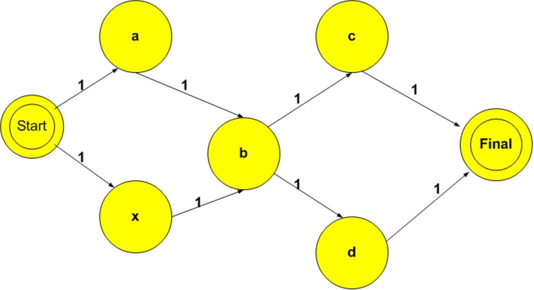
Loss of accuracy in Markov chain.

The problem lies with shared state “b” which has the property that its in-degree and out-degree are both greater than 1. When this occurs, the Markov chain will identify more sequences than were learned. To address this problem state cloning (duplicating the shared state) is traditionally used to address the issue as shown in Fig. 2.

Fig. 2.

State cloning.

However, traditional state cloning is not always sufficient to address situations were multiple states are shared as shown in Fig. 3.

Fig. 3.

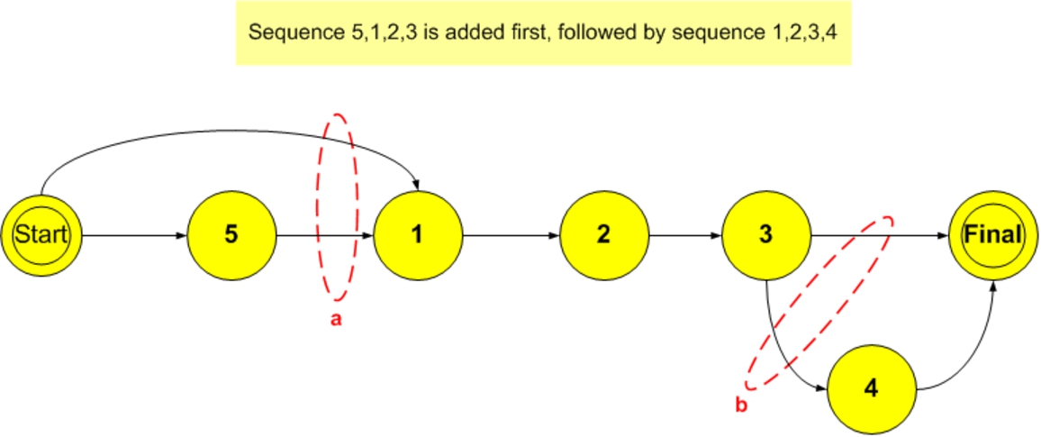
Limitations of state cloning.

The Markov chain in Fig. 3 originally learned sequences $⟨ 5, 1, 2, 3 ⟩$ and $⟨ 1, 2, 3, 4 ⟩$ yet two more sequences are identified. Note that the single node cloning conditions are not violated, yet this graph produces two sequences that were never learned: 1, 2, 3 and 5, 1, 2, 3, 4. In this case, the problem occurs at the transitions covered by points a and b. These transitions allow the generation through shared nodes 1 and 3 of more than 2 sequences. Namely: $⟨ 1, 2, 3, 4 ⟩$ , $⟨ 1, 2, 3 ⟩$ , $⟨ 5, 1, 2, 3 ⟩$ , $⟨ 5, 1, 2, 3, 4 ⟩$ . To address this problem the state cloning approach is extended to cover sequences of shared states such that sequence cloning is needed when the first shared node in a sequence of shared nodes has an in-degree greater than 1 and the last shared node in a sequence of shared nodes has an out-degree also greater than 1. By duplicating all shared states we solve the problem as shown in Fig. 4. Note that both state and sequence cloning increase accuracy but also increase the number of nodes in a Markov chain.

This study introduces the idea of accurately matching a learned timed sequence (context) loosely not necessarily exactly using a combination of longest common subsequence and longest common substring calculations instead of matching “exactly” the context of learned sequences stored in variable order Markov chains.

Fig. 4.

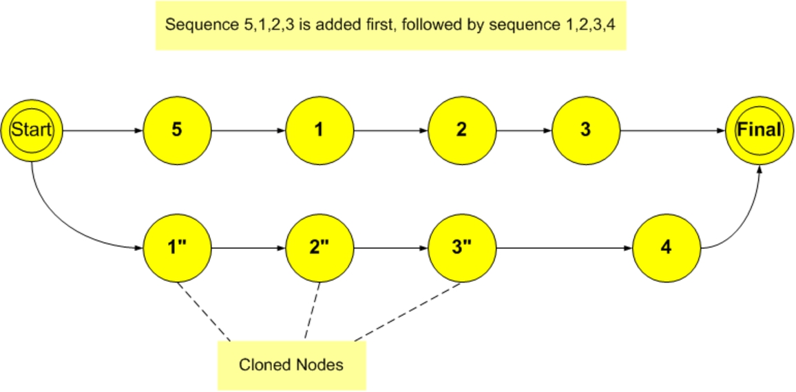
Sequence cloning.

While use of timed sequences of visited web destinations allows increasing the discriminating power of the solution, there still is a need to link up multiple user sessions (sequences) in order to address the poor scalability problem faced by behavioral based identification techniques that forgo the use of a tracking identifier like the source IP address. In this study, hierarchical temporal memories (HTMs) are used to address this need.

A Hierarchical Temporal Memory (HTM) is a technology that is modeled on the algorithms used in the neocortex of the brain [19,23]. Network nodes in an HTM, are organized in a hierarchical way, with each node implementing learning and memory functions. Hierarchical Temporal Memories are an appropriate tool to study complex networks. HTMs perform well when the data they process support a hierarchical structure. Ravasz and Barabasi [40] show that the scale free and high degree of clustering of complex networks like the World Wide Web are the consequence of a hierarchical organization. They show that a small group of nodes, such as communities of interest in the WWW, organize in a hierarchical manner forming larger groups, while still maintaining a scale free topology. This self-similar nesting of different groups into other groups forces a hierarchical structure that well fits the ability of HTMs to correlate groups that are close in space and time. For more information on why HTMs were chosen to deal with complex networks see Appendix G.

3.1. HTM inputs

The next few sections will introduce many terms, computations and symbols which are defined in Appendix I. Figure 7 shows a typical HTM with its inputs. Input sequence ( $IS$ ) is the input sequence being matched by a given HTM layer. For HTM layer 1, $IS$ is a sequence of web destinations (in a real cellular network these are extracted from HTTP requests) and for HTM layers 2 and 3 it is a sequence of temporal groups (variable order Markov chains) matched in the layer below. At layer 1, input is of the form: $Timestamp ⟨ TS, Dest ⟩$ where the format of this input is fully described in Section 3.1.1.

At HTM layers 2 and 3 input is of the form: $λ_{L x} ⟨ {FFB}_{g i}, {FFB}_{g i + 1}, {FFB}_{g i + 2}, \dots ⟩$ where $2 ⩽ x ⩽ 3$ represent layers above the first HTM layer and $1 ⩽ i ⩽$ the number of Markov chains at HTM layer $L_{x - 1}$ . $λ_{L x}$ is a vector of feed forward beliefs, which measures how well inputs match learned sequences and is a vector where only one index is filled based on which temporal group $g i$ matched the input at the lower layer $L_{x - 1}$ of the HTM. The $λ_{L x}$ vector represents the input for HTM layers 2 and 3 where the index of the entry in the vector that is filled represents the feed forward belief of the specific temporal group $g i$ received from lower HTM layers. For instance, vectors $λ_{L 2} ⟨ 0, 0.4, 0 ⟩$ and $λ_{L 2} ⟨ 0.8, 0, 0 ⟩$ , show layer 2 of the HTM receiving from layer 1 a sequence of temporal groups $S_{g 21} (g 2, g 1)$ with feed forward belief values of 40% and 80% for temporal groups 2 and 1 respectively.

3.1.1. Session identification

In this study, the TCP timestamp TS value [29] is used to identify and track user sessions only during the training phase of experiments. The use of TCP timestamps was inspired by the work of Kohno, Broido and Claffy [30]. These authors proposed device recognition by fingerprinting devices via detection of changes in clock skews among different devices using the TCP Timestamp option. Kohno et al., believe that their approach can be used to identify the same physical device among a large number of devices since there exist variability in the clock skew of different physical devices, and it holds that the clock skew for a given device is constant and independent of network access technology. This approach differs from the way in which TCP timestamps are used in this study, where they are leveraged to track directly user sessions and consider clock skew not as a unique fingerprint for devices but instead noise that will decrease the tracking capabilities of this session identification approach. In general, any fingerprinting approach which identifies a logical source (e.g. source IP address) or a physical device as done in Kohno et al. suffers in deployments which obfuscate the source. This becomes particularly problematic in session identification when trying to link up TCP packets belonging to the same user. Consider fingerprinting a device as proposed in Kohno et al. which requires the TCP timestamp value to be passed unchanged through a middle box. Many middle boxes deployed in cellular networks act as “proxies” by splitting the TCP connection between the device and the origin server into two separate TCP connections which cause the origin server to negotiate TCP timestamp options with the middle box instead of the device [28]. This causes the middle box to be mistaken for the real source. This is not a problem when TCP timestamps are used for session identification as proposed in this study. The ability to link up TCP packets belonging to the same user during training will not be impacted whether tapping of communication traffic occurs between device and middle box or middle box and origin server. This is because this approach does not track the source but connections and in this case both connections are surrogates for the single end to end connection between device and origin server. We are not aware of other work that leveraged TCP timestamps to track communication sessions as was done for this study.

Training of HTMs is completely unsupervised and leverages the tracking strength of the TS value to identify consecutive web visits as belonging to the same user session (observation). This is different from the supervised training approach used by Yang in her experiments where a label (user-id) was used to train her inference model. During training, in this study, session identification and user identification are one and the same. During the inference stage the assumption that a specific session belongs to a given user no longer holds and instead the TS value is only used to identify an anonymous session (a set of consecutive web visits belonging to an unknown user that make up an observation). The task of assigning an anonymous session to a specific user is carried out by the Markov chains performing inference within the different layers of each HTM based on past learned patterns of users’ sessions (web visits). All HTMs attempt to recognize each anonymous session and only one HTM will be able to recognize it better than the other HTMs based on its past training.

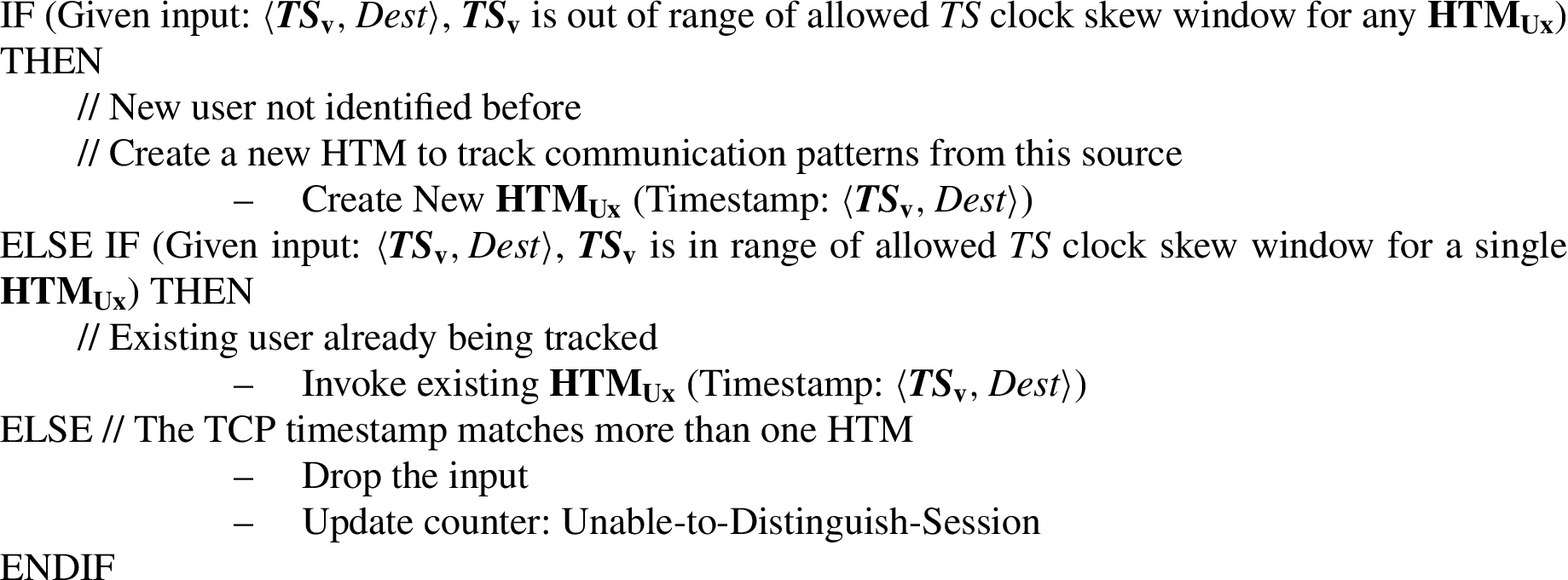
Beacken et al. [6] have discovered that the TCP Timestamp field used for iPhones always starts at the same date/value when the device is restarted but for android devices, the TCP timestamp value on device power up is random. They state that this allows one to be able to distinguish iPhones from android type devices. In this study, the TCP time stamp value, a 32 bit value, which implements a virtual clock on each device, is used to uniquely identify unique sessions associated with a given user. The prototype built for this study identifies multiple communication sessions during the training phase of learning that belong to different users by tracking the unique TS value (TS) of each device. During training, all communication input associated with a given $⟨ TS ⟩$ value within a given time window is fed to a hierarchical temporal memory (HTM) to identify the communication patterns associated with sessions belonging to different users. These communication patterns are defined in terms of the destinations (Dest, a number mapping to the IP address of the web site) visited by this user. The timestamp, calculated from the input at HTM layer 1, has a resolution of 1 millisecond and represents the passage of time with respect to the arrival of input to the HTM. The time stamp is specifically needed to distinguish multiple $⟨ TS, Dest ⟩$ input pairs immediately following each other with potentially the same TCP time stamp values, as either all arriving at the same time or at different times.

The algorithm in Fig. 5 was used to implement communication session identification during the training phase of classification and selection of appropriate HTMs to perform communication pattern identification.

Each ${HTM}_{Ux}$ once created runs a virtual clock with a 1 ms resolution used to track the TS value of sessions associated with this HTM. The allowed TS clock window was computed as follows: $Allowed-TS-Clock-Window = [{TS}_{v} + Clock ()] \pm Clock-Skew-Factor$ . The computation ${TS}_{v} + Clock ()$ needs to account for wrap around at $2^{32}$ . The Clock-Skew-Factor is a fixed maximum allowed clock skew.

Unfortunately, using a fixed window offset from the currently received TCP TS counter to measure clock skew, can potentially either underestimate (lose a single tracked user session) the clock skew with a window that is too small or overestimate (identify a single user session as belonging to multiple user sessions) the clock skew with a window that is too large. A possible way to address this problem is to allow for dynamic resynchronization of the HTM TS counter with a tracked source based on how much of an offset (within a window) a given new received TCP timestamp is from the existing HTM TS counter. This approach would use the new TCP time stamp received as the new TS counter value each time the new TS value is within the window but does not match exactly the current HTM TS counter. This could address the potential increase in clock skew that occurs over time overcoming the limitations of a fixed HTM TS counter. With this newly proposed approach, it will be possible to use a small window size since the algorithm is able to adjust to clock skew over time. The benefit of this approach, as well as determining the best size for the clock skew window, is an area of further research that should be based on the empirical results of studying the characteristics of clock skew of mobile devices in real mobile networks.

Fig. 5.

TCP timestamp session identification algorithm.

3.2. How the HTM works

Each HTM learns and then performs inference. Learning occurs in an unsupervised manner, starting from the bottom layer of the HTM, one layer at a time. Layer 1 learns first. After that, layer 2 learns and once layer 2 is done learning layer 3 completes learning. During training a new HTM is created for each user each time a not seen before user session (based on TCP timestamp tracking) is encountered. Learning entails both spatial and temporal learning. Spatial learning at layer 1 covers identification of individual sequences of web destinations, while at layer 2 and 3 it covers identification of individual sequences of coincidences (temporal groups representing Markov chains matched from the layer below).

Initial learning is completed at each HTM layer with creation of a single Markov graph representing all learned sequences within that HTM layer. At the end of training this single graph is split into many variable order Markov chains by merging all nodes that are most highly connected into one of several Markov chains based on a depth first traversal of the Markov graph (see Fig. 6) thus ensuring that sequences are maintained and not broken up and that sequences held in Markov chains do not overlap.

Fig. 6.

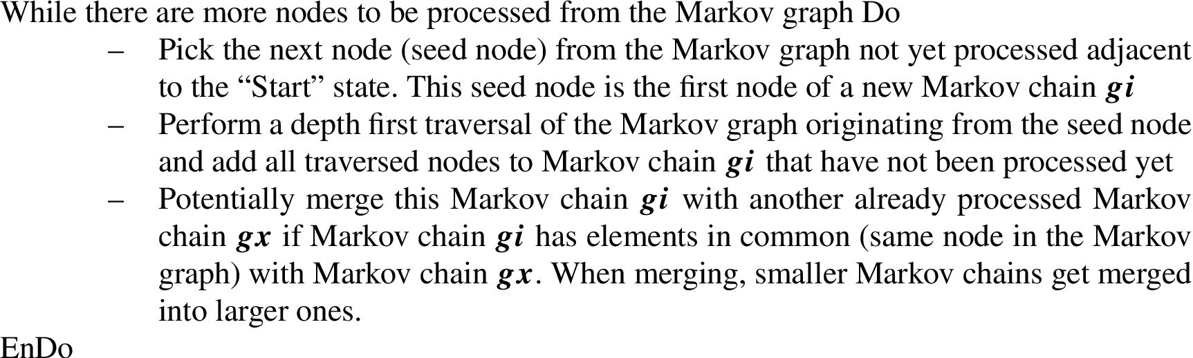
Algorithm to create Markov chains from a single Markov graph.

These Markov chains represent destinations or coincidences (temporal groups) that are highly temporally correlated based the specific temporal order in which they follow each other.

After learning is completed at a given HTM layer, playback occurs. During playback, each HTM at layer $L_{n}$ which completed learning is used to bootstrap learning for the layer above $L_{n + 1}$ using the already learned sequences at layer $L_{n}$ . Playback (an approach introduced in this study) improves the time it takes to train the HTM and allows higher layers to learn higher level concepts that are consistent with the lower level concepts learned by the layers below. In the playback stage, learned sequences at layer n are generated in increasing order of time, so that layer $n + 1$ can correctly learn higher level concepts from the layer below. This in effect simulates the HTM been retrained on the same input used to train the layer below. In order to generate sequences in increasing time order (from oldest to most recent), each node in the Markov graph holds a FIFO queue of timestamps. Each time stamp represents the time when a node was created or modified by updating or adding incoming or outgoing links to/from this node. Time ordered sequence generation is achieved by traversing the Markov graph at each layer of the HTM, starting from the “start” state, while removing from the front of the FIFO queues timestamps associated with nodes with the least recent (oldest) timestamp for each transition up to the “final” state.

During inference the HTM layer collects input until a sequence is formed. The spatial and temporal poolers at each layer of the HTM ensure that sequences are created so that nodes that follow each other in space (sequential order of inputs) and time (timely order of inputs) are grouped together creating a sequence matched against learned sequences of coincidences (stored within variable order Markov chains $g i$ ). The HTM spatial and temporal poolers terminate a sequence and start another under one of the following terminating conditions: (TC₁) A fixed maximum input size has been processed. (TC₂) A maximum learned inter destinations arrival rate is exceeded. (TC₃) The same destination is already present in the sequence (HTM version 1). Note that only HTM layer 1 uses terminating condition TC₂.

Each HTM layer matches the input sequence collected against learned sequences held in Markov chains and finds the best (longest) matching learned sequence (LLS). Each HTM layer computes the feed forward belief (λ) of the best matching learned sequence (LLS). This feed forward belief combines the degree of membership (how well input matches learned sequences) and persistence (how often a matched learned sequence is visited). Belief propagation occurs when HTM layer n passes as input the feed forward belief (λ) to HTM layer $n + 1$ . Belief propagation for casual (Bayesian) networks was first proposed by Judea Pearl [36] and then adapted to HTMs by Deleep George [19].

The output that is sent to the Max Output Layer (see Fig. 8) from each HTM includes identification of the specific HTM and provides the feed forward belief of the matched observation input across all layers of that HTM. The Max Output Layer aggregates the feed forward beliefs ( $λ_{Output}$ ) of up to one observation worth of data (50 web sites) from each HTM using one of seven HTM algorithms and then selects the HTM (user) with the maximum aggregated feed forward belief value among all HTMs as the one that best matches the HTM layer 1 input.

HTMs use one of seven algorithms proposed in this study (detailed in Section 3.5) to aggregate feed forward beliefs and to determine how well an observation matches HTMs’ learned input. Each one of the seven different HTM algorithms (based on the HTM layer where they are applied 1 or 3) combines feed forward beliefs associated with a given input observation based on one of three generic algorithms: average, weighted sum and path probability. The average based algorithm simply computes the averages of feed forward beliefs associated with a given observation. Weighted sum algorithms (BottomUp and TopTop) use weights proportional to the size of an observation matched by a given feed forward belief. The BottomUp algorithm aggregates the feed forward belief with weights proportional to an observation at layer 1 so that the degree of membership calculation at higher layers will be impacted by this weight as the feed forward belief travels up the HTM layers (see Table 1). The TopTop algorithm aggregates the feed forward belief with weights proportional to an observation matched at layer 3. The Path Probability algorithm leverages the idea of independence among feed forward beliefs and simply multiplies together the feed forward beliefs belonging to a given observation.

Fig. 7.

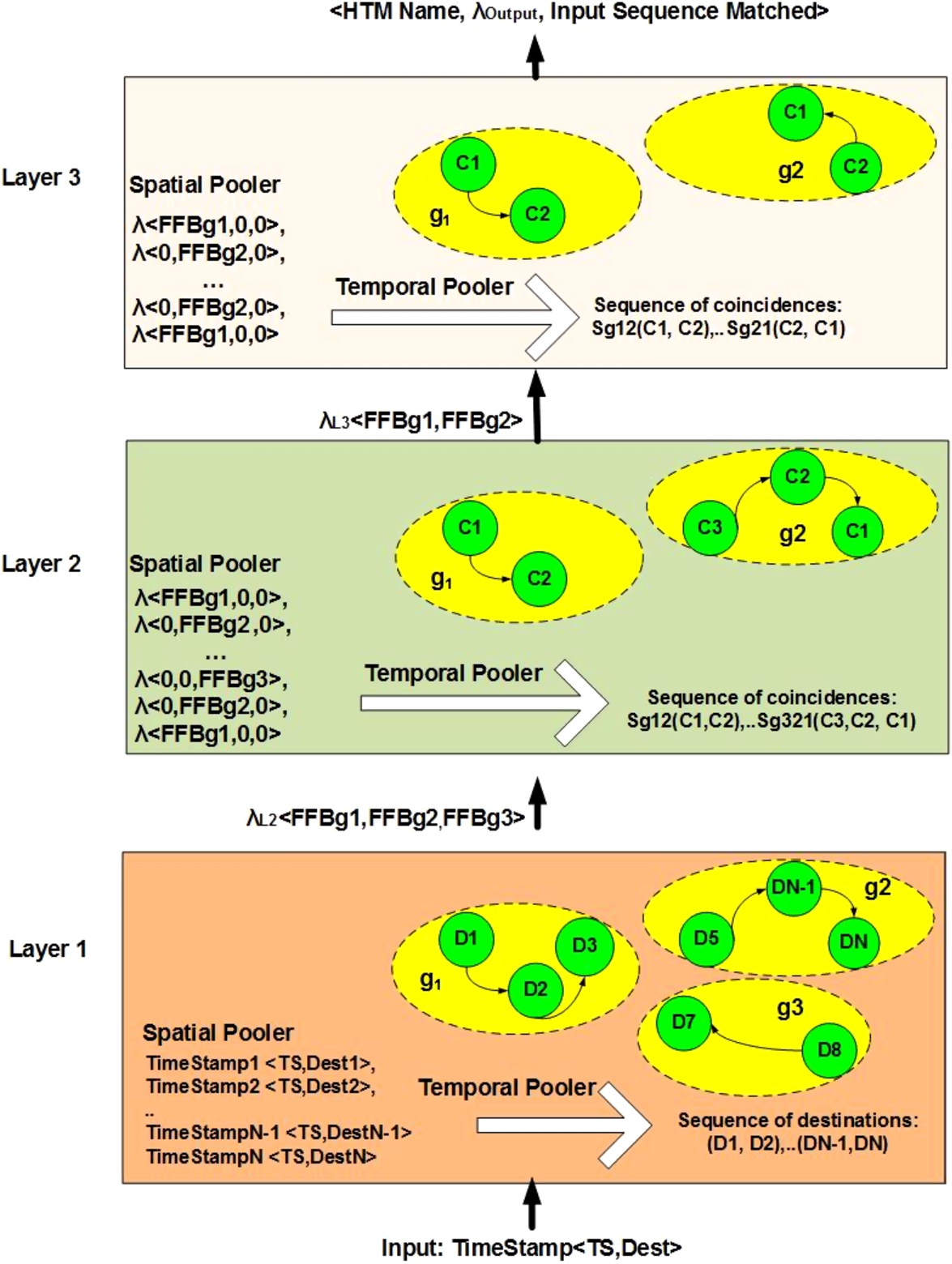
Hierarchical temporal memory layers.

3.3. Feed forward belief calculations

As shown in Fig. 7 the key computation performed by HTMs creates groups of feed forward beliefs ( $λ ⟨ FFBs ⟩$ ) that match the input presented to each HTM layer. The idea is to find the longest learned sequence (LLS) out of all the learned sequences in all of the Markov chains in a given HTM layer which best matches (has the highest degree of membership ( $DM$ ) as shown in Eq. (8)) the input sequence ( $IS$ ). The calculation of $DM$ and persistence ( $SP$ Eq. (7)) of the matched LLS represents how well inferred input ( $IS$ ) is matched against learned input. In terms of notation: (Abbreviation) Function name( $Arg 1, \dots, Arg n$ ) represents a function “Function name” which takes n arguments $Arg 1, \dots, Arg n$ and is referenced using the abbreviated name “Abbreviation”. The rest of this section presents the key calculations necessary to compute feed forward beliefs (Eqs (9) and (10)) that are calculated within each HTM layer before being propagated up to next layer. Refer to Appendix I for specific explanations of abbreviations used in this section. $\begin{array}{l} (ALLLS_Cond) Adjusted Length LLS Condition (IS, cLLS) \\ = if IS is a substring of cLLS and {IS}_{1} = {cLLS}_{1} and | cLLS | > | IS |, \\ (ALLLS) Adjusted Length LLS (IS, cLLS) = \{\begin{matrix} | IS |, & ALLLS_Cond, \\ max (| IS |, | cLLS |), & otherwise, \end{matrix} \\ (1) & ({LCS}_{m}) Longest Common Subsequence Measure (IS, cLLS) = \frac{| LCS (IS, cLLS) |}{ALLLS (IS, cLLS)}, \\ (2) & ({LCSU}_{m}) Longest Common Substring Measure (IS, cLLS) = \frac{| {LCS}_{u} (IS, cLLS) |}{ALLLS (IS, cLLS)} . \end{array}$

See Appendix C for an example of how to use Eqs (1) and (2). $\begin{array}{l} (Fq) Frequency of visits ({cLLS}_{i}) \\ = number of times {cLLS}_{i} occurs in Markov chain g i \\ (3) & within this HTM layer across all Markov chains in that HTM layer, \\ NLS = number of all learned sequences within a given HTM layer, \\ (4) & (Ps) Persistence (cLLS) = \frac{Fq (cLLS)}{NLS}, \\ Similarity Weights = Ws + Wu + Wp = 1.0, \\ (5) & where in this study Ws = 0.495, Wu = 0.495, Wp = 0.01, \\ (SS) Sequence Similarity (IS, cLLS) \\ (6) & = ({LCS}_{m} (IS, cLLS) \times Ws) + ({LCSU}_{m} (IS, cLLS) \times Wu), \\ (7) & (SP) Sequence Persistence (cLLS) = (Ps (cLLS) \times Wp), \\ (8) & (DM) Degree of Membership (IS, cLLS) \\ (8a) & = max_{LLS} (SS (IS, cLLS)) when | \forall s, SS (IS, cLLS) > SS (IS, s) | = = 1, \\ (8b) & = max_{LLS} (SS (IS, cLLS), SP (cLLS)) when | \forall s, SS (IS, cLLS) > SS (IS, s) | > 1, \\ where s = all learned sequences, including cLLS, in a given HTM layer . \end{array}$

The best matching LLS is that candidate LLS (cLLS), in a given HTM layer, that has the maximum degree of membership value when measured against the input sequence ( $IS$ ). For instance, assume $IS = ⟨ S_{1}, S_{3} ⟩$ which matches ${cLLS}_{1} ⟨ S_{1}, S_{2}, S_{3}, S_{4} ⟩$ and ${cLLS}_{2} = ⟨ S_{1}, S_{3}, S_{6} ⟩$ in Fig. 14, then LLS which satisfies $DM (IS, cLLS)$ is ${cLLS}_{2}$ since: $\begin{array}{l} {LCS}_{m} (IS, cLLS) = {LCS}_{m} (IS, {cLLS}_{2}) = 2 / 2, \\ {LCSU}_{m} = (IS, cLLS) = {LCS}_{u} (IS, {cLLS}_{2}) = 2 / 2, \\ {LCS}_{m} (IS, cLLS) = {LCS}_{m} (IS, {cLLS}_{1}) = 2 / 4, \\ {LCSU}_{m} = (IS, cLLS) = {LCS}_{u} (IS, {cLLS}_{1}) = 1 / 4, \\ SS (IS, {cLLS}_{1}) = (0.5 \times 0.495) + (0.25 \times 0.495), \\ SS (IS, {cLLS}_{2}) = (1 \times 0.495) + (1 \times 0.495), \\ SS (IS, {cLLS}_{2}) > SS (IS, {cLLS}_{1}) then based on (8a) max_{LLS} (SS (IS, cLLS)) is {cLLS}_{2} . \end{array}$

When more than one cLLS sequence exists with the same maximum sequence similarity values then the more persistent of these cLLS sequences is chosen. Consider a different example where $IS = ⟨ S_{1}, S_{6} ⟩$ and from Fig. 14 ${cLSS}_{1} = ⟨ S_{1}, S_{8}, S_{6} ⟩$ and ${cLSS}_{2} = ⟨ S_{1}, S_{3}, S_{6} ⟩$ , in this case Eq. (8b) is used since two sequences have the same sequence similarity values, namely $| SS (IS, {cLLS}_{1}) = SS (IS, {cLLS}_{2}) | > 1$ . In this case, $LLS = ⟨ S_{1}, S_{3}, S_{6} ⟩$ since $SP ({cLLS}_{2}) = 2 / 16 > SP ({cLLS}_{1}) = 1 / 16$ . $\begin{array}{l} (FFB) Feed Forward Belief (IS, LLS) \\ (9) & = min (1.0, DM (IS, LLS) + SP (LLS)) where min is the minimum function. \end{array}$ $FFB (IS, LLS)$ is the feed forward belief used with all HTM algorithms except for path probability. The feed forward belief applied with the path probability HTM algorithm (see Section 3.5 for details) is shown below: $\begin{array}{rcl} (FFB_PP) Path Probability of LLS (LLS) \\ = P (LLS) = P ({LLS}_{1}) \times P ({LLS}_{2} | {LLS}_{1}) \times P ({LLS}_{3} | {LLS}_{1} {LLS}_{2}) \times \dots \\ (10) & \times P ({LLS}_{n} | {LLS}_{1} \dots {LLS}_{n - 1}), \end{array}$ where: $\begin{matrix} (11) & P ({LLS}_{1}) = \{\begin{matrix} \frac{Fq ({LLS}_{1})}{NLS}, & if {LLS}_{1} = {IS}_{1}, \\ penalty = 0.0001, & otherwise, \end{matrix} \end{matrix}$ where penalty is an error probability for mismatches against $IS$ . $\begin{matrix} (12) & \begin{matrix} Fq ({LSS}_{j \to k}) = frequency of visits across node transition j \to k, \\ P ({LLS}_{k} | {LLS}_{j}) = \frac{Fq ({LLS}_{j \to k})}{Fq ({LLS}_{j})} where k, j > 1 . \end{matrix} \end{matrix}$

3.4. Feed forward belief propagation calculations

Feed forward beliefs propagate through HTM layers, as shown in Fig. 7, following the formulas shown in Table 1. Feed forward beliefs exiting the output (last) HTM layer will be directed to the Max HTM Output Layer, shared across all HTMs, which aggregates feed forward beliefs for an each observation worth of inputs (see Fig. 8).

Table 1
Feed forward beliefs for each HTM layer

HTM layers Feed forward beliefs propagation

Max HTM Output Layer output $(OR) Observation Result = ⟨ HTM_name, MAX_FFB_HTMs, Observation input ⟩$ , HTM_name is the name of the HTM matching Observation input with the highest aggregated feed forward belief value computed using MAX_FFB_HTMs for $S_{λ Output k \dots k + N}$ over all HTMs

${HTM}_{1 \dots M}$ layer 3 output/Max HTM Output Layer input $\begin{matrix} (13) & λ_{Output} = \{\begin{matrix} FFB_{PP}_{g k} (LLS) \times ({IAL}_{S g j \dots j + N}), \\ if HTM algorithm is Path Probability \\ {FFB}_{g k} (S_{g j \dots j + N}, LLS) \times ({IAL}_{S g j \dots j + N}), \\ otherwise, \end{matrix} \end{matrix}$ where $1 ⩽ k ⩽$ number of Markov chains at HTM layer 3. Note that when the HTM is configured with only 1 layer then $λ_{L 2} = λ_{Output}$

${HTM}_{1 \dots M}$ layer 2 output/ ${HTM}_{1 \dots M}$ layer 3 input $\begin{matrix} (14) & λ_{L 3} = \{\begin{matrix} FFB_{PP}_{g j} (LLS) \times ({IAL}_{S g i \dots i + N}), \\ if HTM algorithm is Path Probability, \\ {FFB}_{g j} (S_{g i \dots i + N}, LLS) \times ({IAL}_{S g i \dots i + N}), \\ otherwise, \end{matrix} \end{matrix}$ where $1 ⩽ j ⩽$ number of Markov chains at HTM layer $L_{2}$

${HTM}_{1 \dots M}$ layer 1 output/ ${HTM}_{1 \dots M}$ layer 2 input $\begin{matrix} (15) & λ_{L 2} = \{\begin{matrix} {FFB}_{g i} (IS, LLS) \times (\frac{| IS |}{OS}), \\ if HTM algorithm is BottomUp, \\ FFB_{PP}_{g i} (LLS), \\ if HTM algorithm is Path Probability, \\ {FFB}_{g i} (IS, LLS), \\ otherwise, \end{matrix} \end{matrix}$ where $1 ⩽ i ⩽$ number of Markov chains at HTM layer $L_{1}$ and observation size (OS) is 50

${HTM}_{1 \dots M}$ layer 1 input received from the network $Timestamp ⟨ TS, {Dest}_{1} ⟩ \dots Timestamp ⟨ TS, {Dest}_{N} ⟩$

HTM layers	Feed forward beliefs propagation
Max HTM Output Layer output	$(OR) Observation Result = ⟨ HTM_name, MAX_FFB_HTMs, Observation input ⟩$ , HTM_name is the name of the HTM matching Observation input with the highest aggregated feed forward belief value computed using MAX_FFB_HTMs for $S_{λ Output k \dots k + N}$ over all HTMs
${HTM}_{1 \dots M}$ layer 3 output/Max HTM Output Layer input	$\begin{matrix} (13) & λ_{Output} = \{\begin{matrix} FFB_{PP}_{g k} (LLS) \times ({IAL}_{S g j \dots j + N}), \\ if HTM algorithm is Path Probability \\ {FFB}_{g k} (S_{g j \dots j + N}, LLS) \times ({IAL}_{S g j \dots j + N}), \\ otherwise, \end{matrix} \end{matrix}$ where $1 ⩽ k ⩽$ number of Markov chains at HTM layer 3. Note that when the HTM is configured with only 1 layer then $λ_{L 2} = λ_{Output}$
${HTM}_{1 \dots M}$ layer 2 output/ ${HTM}_{1 \dots M}$ layer 3 input	$\begin{matrix} (14) & λ_{L 3} = \{\begin{matrix} FFB_{PP}_{g j} (LLS) \times ({IAL}_{S g i \dots i + N}), \\ if HTM algorithm is Path Probability, \\ {FFB}_{g j} (S_{g i \dots i + N}, LLS) \times ({IAL}_{S g i \dots i + N}), \\ otherwise, \end{matrix} \end{matrix}$ where $1 ⩽ j ⩽$ number of Markov chains at HTM layer $L_{2}$
${HTM}_{1 \dots M}$ layer 1 output/ ${HTM}_{1 \dots M}$ layer 2 input	$\begin{matrix} (15) & λ_{L 2} = \{\begin{matrix} {FFB}_{g i} (IS, LLS) \times (\frac{\| IS \|}{OS}), \\ if HTM algorithm is BottomUp, \\ FFB_{PP}_{g i} (LLS), \\ if HTM algorithm is Path Probability, \\ {FFB}_{g i} (IS, LLS), \\ otherwise, \end{matrix} \end{matrix}$ where $1 ⩽ i ⩽$ number of Markov chains at HTM layer $L_{1}$ and observation size (OS) is 50
${HTM}_{1 \dots M}$ layer 1 input received from the network	$Timestamp ⟨ TS, {Dest}_{1} ⟩ \dots Timestamp ⟨ TS, {Dest}_{N} ⟩$

The input activation level equation shown below measures the strength of a match between input and learned sequences and is further defined in Appendix I. $\begin{array}{l} ({IAL}_{S g i \dots i + N}) Input Activation Level (S_{g i \dots i + N}, {FFB}_{g i}) \\ (16) & = min (1.0, \frac{\sum_{i = 1}^{| S_{g i \dots i + N} |} {FFB}_{g i}}{| S_{g i \dots i + N} |}) . \end{array}$

3.5. HTM algorithms calculations

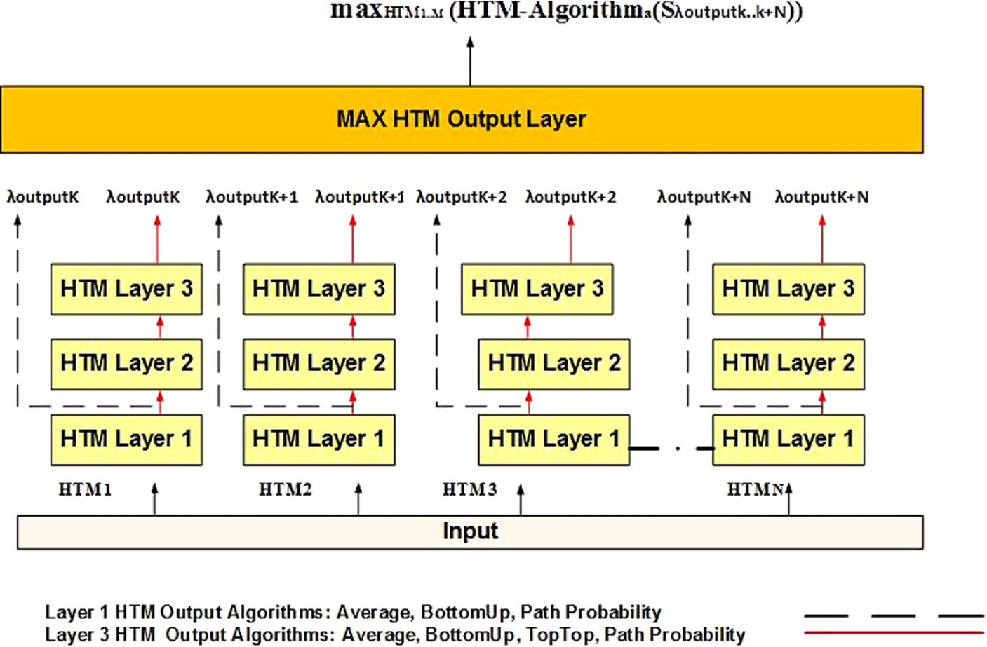
The seven HTM algorithms described in previous sections are implemented based on the three generic algorithms defined by equations 18, 19 and 20. The algorithms are deployed mainly in the Max Output Layer and also across the HTM layers for the Path Probability and BottomUp algorithms. Figure 8 shows $λ_{Output}$ which represents the feed forward belief output from layer 3 of an HTM to the Max Output Layer and $S_{λ Output k \dots k + N}$ which is a sequence of such feed forward beliefs. These parameters are used by the Max Output Layer to compute the highest valued feed forward belief for a given observation using the formula shown below. $\begin{array}{l} (MAX_FFB_HTMs) Max Feed Forward Belief for HTMs (S_{λ Output k \dots k + N}) \\ (17) & = max_{HTM 1 \dots M} ({HTM_Algorithm}_{a} (S_{λ Output k \dots k + N})), \end{array}$ where a is one of 3 generic HTM algorithms (Average, Weighted Sum, Path Probability), $1 ⩽ M ⩽$ number of HTMs/users learned during training, ${HTM}_{1 \dots M}$ is the name of all HTMs learned during training.

Fig. 8.

HTM Max Output Layer inputs and output.

The three generic HTM algorithms which process feed forward beliefs within the Max HTM Output Layer are shown below: $\begin{array}{l} NB = | S_{λ Output k \dots k + N} | is the number of beliefs per observation, \\ (18) & Average (S_{λ Output k \dots k + N}) = (\sum_{k = 1}^{NB} λ_{Output k}) / NB, \\ (19) & Weighted Sum (S_{λ Output k \dots k + N}, {IS}_{k}, OS) = \sum_{k = 1}^{NB} (λ_{Output k} \times \frac{| {IS}_{k} |}{OS}), \end{array}$ where ${IS}_{k}$ is HTM layer 1 input sequence associated with $λ_{Output k}$ and $OS$ = observation size (50 web destinations at HTM layer 1) $\begin{matrix} (20) & Path Probability (S_{λ Output k \dots k + N}) = \prod_{k = 1}^{NB} λ_{Output k} . \end{matrix}$

See Appendix E for an example on how the Max HTM Ouput Layer utilizes HTM algorithms. Table 2 provides more details about which HTM layer provides inputs to the Max output layer for specific HTM algorithms.

Table 2

HTM Algorithms

HTM algorithms	HTM generic algorithms ( ${HTM_Algorithm}_{a}$ )	HTM layers supplying input to Max HTM Output
Average	Average	1, 3
TopTop	Weighted Sum	3
BottomUp	Average	1, 3
Path Probability	Path Probability	1, 3

How to read Table 2: The Average and BottomUp HTM algorithms use the average generic HTM algorithm with inputs to Max HTM Output Layer from HTM layers 1 and 3 (see Fig. 8). The TopTop HTM algorithm uses the weighted sum algorithm with inputs exclusively from layer 3. Allowing HTM algorithms to generate inputs from either HTM layer 1 or 3 was done to enable verification of HTMs with and without HTM hierarchies. The BottomUp algorithm, takes the average of feed forward beliefs at the Max HTM Output Layer computed using the weighted sum at layer 1 (see Table 1, Eq. (15)). This was done to normalize differences in calculations due to large number of beliefs produced from layer 1 versus the few number of beliefs produced from layer 3 of HTMs.

4. Experiments

The HTM together with the entire set of tools needed to support the experiments conducted in this study were developed from scratch in Java. It became critical then to qualify the HTM to guarantee its correct implementation before performing any experiments. A “calibration” procedure was used to ensure that experiments run using all seven HTM algorithms, as well as, all alternate Markov chain based algorithms would be able to recognize users using their own trained data set instead of a different test data set, achieving in the case of synthetic data sets, 100% recall accuracy results. This initial calibration criterion was used to qualify each one of the HTMs and alternate Markov chains algorithms as being correctly implemented with respect to their ability to accurately train and infer their own input. It became also important to create reference data sets for the experiments themselves, allowing validation of the algorithms against a well understood baseline. For this purpose synthetic data sets were created (see Appendix F for a description of how synthetic data was created to be as close as possible to real network data). Only if the HTM and alternate Markov chain algorithms could achieve high levels of recall accuracy with these synthetic data sets would a corresponding new set of experiments be conducted with real network data extracted from an operator cellular network. In this study a total of 514 experiments were conducted utilizing synthetic data and 228 experiments utilizing real network data.

Table 3
Fourteen sets of experiment for this study

Experiment types (E_1–14) Data type Number of experiments using HTM algorithms (7) Number of experiments using alternate MC algorithms (4)

(E₁) User identification no concept drift Synthetic 210 120

(E₂) User identification with concept drift Synthetic 84 48

(E₃) User identification under DOS attack Synthetic 21 –

(E₄) User identification under Phish attack Synthetic 21 –

(E₅) HTM accuracy scalability Synthetic 10 –

(E₆) User identification alternate MC Real – 24

(E₇) User identification HTM2++ Real 42 –

(E₈) User identification HTM2 Real 42 –

(E₉) User identification HTM1 Real 42 –

(E₁₀) User identification under DOS attack Real 21 –

(E₁₁) User identification under Phish attack Real 21 –

(E₁₂) Session identification Real 18 –

(E₁₃) User identification continuous learning Real 12 –

(E₁₄) User identification under DOS attack with continuous learning Real 6 –

Experiment types (E_1–14)	Data type	Number of experiments using HTM algorithms (7)	Number of experiments using alternate MC algorithms (4)
(E₁) User identification no concept drift	Synthetic	210	120
(E₂) User identification with concept drift	Synthetic	84	48
(E₃) User identification under DOS attack	Synthetic	21	–
(E₄) User identification under Phish attack	Synthetic	21	–
(E₅) HTM accuracy scalability	Synthetic	10	–
(E₆) User identification alternate MC	Real	–	24
(E₇) User identification HTM2++	Real	42	–
(E₈) User identification HTM2	Real	42	–
(E₉) User identification HTM1	Real	42	–
(E₁₀) User identification under DOS attack	Real	21	–
(E₁₁) User identification under Phish attack	Real	21	–
(E₁₂) Session identification	Real	18	–
(E₁₃) User identification continuous learning	Real	12	–
(E₁₄) User identification under DOS attack with continuous learning	Real	6	–

Table 3 shows the entire set of experiments conducted in this study. All experiments test the ability of the seven HTM algorithms to attribute communication traffic to users under test. In addition, four alternate algorithms based on Markov chains (MC) were also tested (E₁, E₂, E₆) in order to compare the HTM inference recall accuracy performance against traditional algorithms that, like HTM algorithms, recognize sequences leveraging Markov chains. A single experiment usually entails training either the HTM using one of the seven HTM algorithms or training one of four MC algorithms on a specific data set (synthetic or real) to perform a specific experiment such as user identification. User identification experiments with synthetic data sets were performed without noise (E₁) and with noise introduced in the test data set in the form of either concept drift (E₂) or in the form of DOS or Phish attacks (E₃, E₄). The ability to maintain high levels of recall accuracy performance with increasing number of users (E₁, E₅) and increasing number of destinations (E₁) was also measured. Similar experiments were also performed utilizing data sets collected from a real cellular network (E₆–E₁₁). Experiments E₁₃ and E₁₄ verify the ability of the HTM to identify users, utilizing real network data, by continuing to learn during the inference phase of the experiment instead of just learning during the train phase of the experiment. Experiments E₁₂ measure the accuracy of session identification performed during the train phase of user identification experiments.

Markov chain based algorithms were chosen because of Markov chains’ ability to recognize sequences and because the HTM also uses Markov chains, albeit with modifications. The following types of Markov chains (MC) were used to baseline this work: [Fixed Order] 1st Order Markov Chains, [Fixed Order] 3rd Order Markov Chains, [Variable Order] All-K Markov model, where $K = 3$ , [Variable Order] (PPM-C) Prediction by Partial Match, where $K = 3$ .

In this study, mismatches found by MC based algorithms between learned and new input sequences are assigned a fixed penalty when using fixed order Markov chains and a variable penalty proportional to the number of different destinations matched so far and their frequencies when using variable order Markov chains.

4.1. Experiments using synthetic data

Three hundred and thirty experiments (E₁) were conducted using synthetic data without simulating context drift which used 1000, 5000, and 10,000 visited web destinations. These experiments simulated 5, 20, 50, 100, 500 users accessing the network using 5 days’ worth of train data and either one or two days’ worth of test data or just 3 observations (one observation “Obs” equals 50 visited web destinations) worth of test data per user. For instance, Table 21 in Appendix H shows that for 5 users and 1000 visited web destinations, 11 experiments are executed using 5 train days and 1 test day (5/1), 11 experiments using 2 days’ worth of test data (5/2), 11 experiments using 3 observations (3 Obs) worth of test data for a total of 33 experiments. On the other hand for 500 users using 5000 destinations Table 21 shows 11 experiments being executed using 3 observations in the test data set.

All 132 concept drift experiments (E₂) shown in Table 22 in Appendix H involved visits to 1000 web destinations with 5 users, with 5, 10, 15, 20 training days and 2, 3, 4, 5 test days’ worth of test data respectively (see Appendix F for a description of how concept drift was simulated using a random walk algorithm). Concept drift is introduced in the form of 20% new destinations and 10% new transitions between destinations not in the original train data set. The first line of Table 22 represents the baseline (no concept drift).

In this study, users are identified based on their normal behavior and anomalous traffic is introduced as a form of noise to understand how much user identification accuracy is lost when noise (in the form of an attack) is introduced in the normal communication traffic patterns of users. The idea is not to identify the attack traffic but to identify normal traffic (tied to a specific user) in spite of the presence of embedded attack traffic (noise). The assumption is that when noise is introduced in the form of a phish or DOS attack from the device, it is due to the device having been compromised, possibly based on a download of an infected application. As the subscriber uses his mobile device to browse the Internet (normal behavior) the malicious app is at work in the background, launching its phish or DOS attacks. Table 23 in Appendix H shows twenty-one experiments (E₃) which were conducted with HTM algorithms by simulating denial of service attacks, embedded within synthetic network data, where the attack is initiated from individual devices during the test phase to a number of destinations (5, 10, 20) learned at train time. The destinations are attacked repeatedly over time (within a time interval of 5, 10, 20 ms and spaced by a fixed time interval of 5 ms). The idea is to determine how well the HTM can continue to identify users before and after the attack. In these experiments 10 users are used and 4 of them are assumed to be infected and to start DOS attacks during the test phase. The motivation for attacking destinations learned at train time is based on the assumption that perpetrators of DOS attacks typically target sites or services hosted on high-profile web servers such as on-line retailers, banks, credit card payment gateways which are likely to have been visited by the user, thus making the attack less likely to be detected (less conspicuous).

Table 24 in Appendix H shows twenty-one experiments which simulate phishing attacks (E₄), embedded within synthetic network data, which were run using HTM algorithms. For these experiments, attacks are initiated from individual devices during the test phase where unique destinations (1, 3, 5) are randomly selected from outside the user training data set (to simulate access to never visited before web phish sites) and attacked within a time interval (1 ms, 3 ms, 5 ms) spaced by random time intervals (1 min–1 h).

Ten scalability experiments (E₅) were also run using the two best performing HTM algorithms to measure the ability of the HTM to accurately identify users as the number of users increased from 150 to 500 users

4.2. Experiments using real network data

The next set of user identification experiments used real network data collected from a CDMA/LTE cellular data network in North America over a period of approximately a month. Experiments were conducted against HTMs using the following parameters: 5 and 10 users, 5 train days and 1 test day, 5 train days and 2 test days, 10 train days and 3 test days. The actual number of different web destinations visited by all users over the month was: 4903 destinations for 5 train days/1 test day, 5221 destinations for 5 train days/2 test days, 6672 destinations for 10 train days/3 test days.

The data originally collected from the network was for 50 users for a period of one month, unfortunately only 10 users used enough communication data to support the train and test timelines proposed for this study.

One hundred twenty six user identification experiments (E₇, E₈, E₉) were conducted using real network data running seven HTM algorithms. Table 25 in Appendix H shows the configuration for these experiments. For instance, 10 users leveraging 5 days of train data and 1 day worth of test data (5/1).

Twenty four user identification experiments were run using alternate Markov based algorithms (E₆). Forty two experiments (E₉) uncovered shortcomings in the HTM state machines when handling repetitive consecutive web destinations embedded in the real network input data set. The HTM was modified to address these shortcomings and the same 42 user identification experiments (E₈), using the same data set, were run to determine if the HTM accuracy could be improved. Finally, repetitive web destinations occurring at the exact same time (same timestamp) were removed from the input data set and the 42 same user identification experiments were run again (E₇).

Twenty one experiments which identify users in spite of simulated DOS attacks (E₁₀) and 21 experiments which identify users in spite of simulated Phish attacks (E₁₁) were also run using real network data (using parameters shown in Tables 23, 24).

The inability to collect TCP timestamps from the real cellular network limited session identification experiments to utilizing synthetically created TCP timestamps. It thus became necessary to conduct a set of experiments (E₁₂) to determine how noise introduced by different session identification algorithms impacts train data and the ensuing inference accuracy of HTMs. Session Identification experiments were performed by creating training data sets for the HTM that use one of three session identification algorithms: (1) Source IP, (2) Sliding Window, (3) TCP Timestamp. The train data set to be modified by the session identification algorithms uses real network data. The experiments include a preliminary step which runs the session identification algorithms against real network data to produce a new altered train data set that is modified based on the bias introduced by each session identification algorithm run under conditions that introduce noise. The experiment would then train the HTM with this altered train data set and use the original real network data as the test data set. Using the “Source IP” algorithm, all input with the same source IP address belongs to the same user. The “Sliding Time Window” algorithm selects the first (oldest) HTTP request in a time window based on the source IP address and assign it to user-x, then all subsequent HTTP requests within the time window for that source IP address, belong to the same user-x. As long as data is available for user-x within the window over time, then that session belongs to user-x otherwise that session is assigned to a new user (source IP address) selected at random based on users who have data falling within the sliding time window. Note that the sliding window approach presented in other related literature [4,46] only specified that requests occurring together in time belong to the same session. No other detail was given as to how a specific session was identified among others occurring at similar times. Thus, the use of the oldest source IP in a given time window as the seed for identifying a given user is proposed in this paper in support of this approach. The TCP Timestamp algorithm uses the TCP Timestamp values within a clock skew window to track different users.

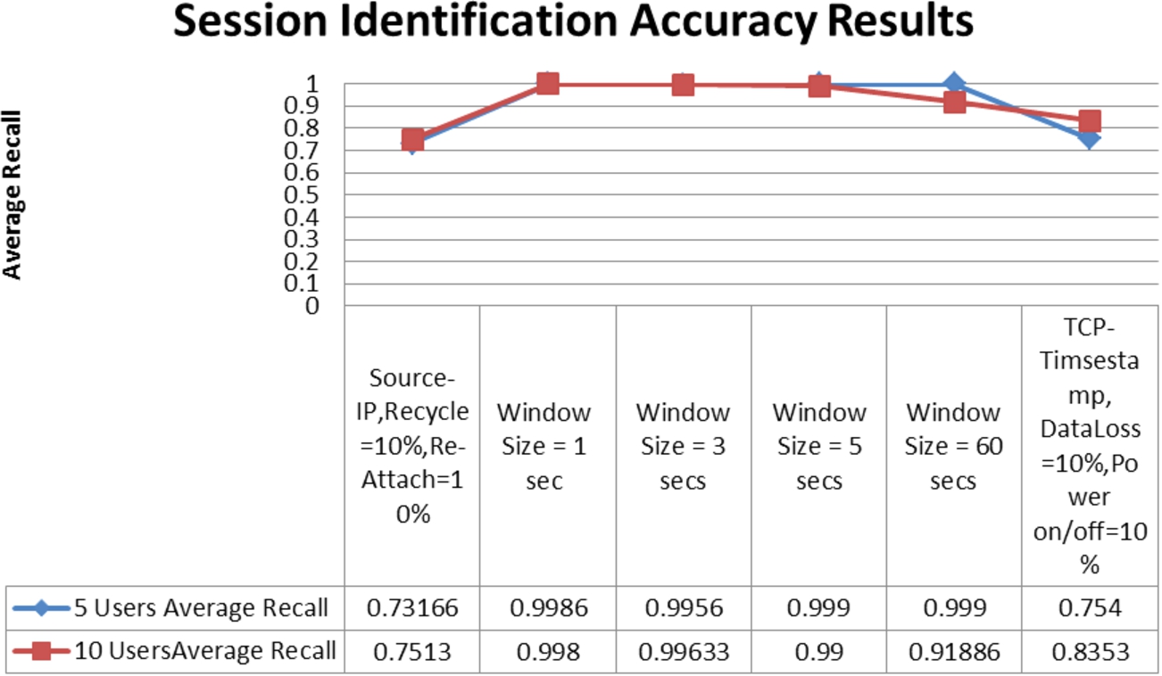
A total of 18 session identification experiments were run where the source IP and TCP Timestamps leveraged real life scenarios to alter the original train data set. This was done by random simulation of recycling of the same source IP address among users as done by NATs and web proxy middle-boxes and by random simulation of re-attachment of a device with a new source IP as done when users move across networks. For TCP Timestamp, data loss was randomly simulated by creating holes in the data stream as well as random simulation of device power off/on. The number of users in these experiments is 5 and 10 for 5 train days, with the following additional experiment parameters: (Source IP): 10% recycle source IP address and 10% access network re-attaches; (Sliding Window): Sliding window size in seconds (1, 3, 5, 60); (TCP Timestamp): 10% data loss and 10% device power on/off.

In order to determine if it was possible to further improve HTM user attribution accuracy with real network data in the presence of real concept drift, continuous learning logic was added to the HTM. Continuous learning was implemented by allowing the output of the Max HTM Output Layer, which identifies which ${HTM}_{x}$ a given observation belongs to, to be sent back to layer 1 of that ${HTM}_{x}$ so that it can learn that observation. ${HTM}_{x}$ then during inference uses a mechanism similar to “playback” to learn the just received observation across all HTM layers. Two types of continuous learning were implemented: (1) Continuous Baseline which lets the Max HTM Output Layer send feedback to the correct HTM that matched the given observation. (2) Continuous Inference which lets the Max HTM Output Layer send feedback to the inferred HTM (which could be right or wrong) that matched the given observation. Twelve user identification experiments (E₁₃) with continuous learning were conducted for 5 and 10 users using the BottomUp approach run at HTM layer 3.

In order to determine if continuous learning could improve the HTM accuracy in spite of DOS or Phish attacks, 6 experiments (E₁₄) were run. These experiments were conducted using real network data for 10 users using 5 days’ worth of train data and 2 days’ worth of test data, using the BottomUp Layer 3 HTM algorithm and applying simulated DOS and Phish attacks configured with the same parameters previously described for these experiments in Tables 23, 24.

5. Results

Due to the large number of experiments conducted for this study only key results will be reported in this section. Following are key findings from these experiments:

HTM algorithms such as BottomUp and TopTop tend to provide the highest levels of recall accuracy and scalability among all HTM algorithms.

The HTM algorithm Path Probability tends to perform the worst among all HTM algorithms.

Alternate Markov chains based algorithms (1st and 3rd Order Markov Chains, All-K and PPM) perform very poorly in terms of recall accuracy and recall accuracy scalability compared to HTM algorithms. However, Alternate Markov chains based algorithms excel at recognizing their own train input.

HTM recall accuracy is strongly influenced by the number of visited web destinations and the pattern of behavior (which web sited are visited) of users, specifically:

Recall accuracy for HTM algorithms improves dramatically moving from 1000 to 5000 web destinations visited by all users. Beyond 5000 web destinations accuracy levels off.

Continuous repetitive patterns (large number of identical web destinations visited over a very short time window) found in real network data impact negatively HTM algorithms’ recall accuracy.

User behavior changes (new web sites visited) from behavior learned at train time (concept drift) do impact negatively HTM recall accuracy. Concept drift that splits randomly learned sequences of web destinations has the most negative impact on HTM recall accuracy performance.

Continuous learning does mitigate the negative impact of concept drift on HTMs’ recall accuracy performance.

Recall accuracy reported by HTM algorithms at layers 1 and 3 is generally comparable.

HTMs tolerate reasonably well noise introduced in test datasets in the form of DOS or Phish attacks.

TCP Timestamps can be effective in session identification, however if noise is present in the training data set, experiments showed that the sliding window algorithm can be a more accurate session identification algorithm.

5.1. Results using synthetic data sets

Based on experiment set (E₁), alternate MC based algorithms with one day worth of test data never produced recall accuracy statistics above 42% (see Table 4 below) and when the test data set consisted of 3 observations, these algorithms never produced recall statistics over 66% (see Table 5). In contrast, HTM algorithms produced accuracy statistics (recall statistics) as high as 99% for a sample of 100 users with one day worth of test data as shown in Table 4 and 99% recall accuracy for a sample of 500 users with 3 observations worth of test data as shown in Table 5.

Table 4
5–100 users, 5000 destinations, 5 train days and 1 test day synthetic data (E₁)

(E₁) HTM and alternate algorithms Variable number of observations per user

5 users, 5000 destinations, 5 train/1 test, ave recall 20 users, 5000 destinations, 5 train/1 test, ave recall 50 users, 5000 destinations, 5 train/1 test, ave recall 100 users, 5000 destinations, 5 train/1 test, ave recall

HTM L₁ simple ave 0.988 0.91 0.918 0.89

HTM L₁ BottomUp 0.99 0.99 0.986 0.96

HTM L₁ Path Probability 0.99 0.98 0.94 0.92

HTM L₃ simple ave 0.988 0.91 0.91 0.89

HTM L₃ BottomUp 0.99 0.99 0.98 0.967

HTM L₃ TopTop 1.00 0.997 0.999 0.986

HTM L₃ Path Probability 0.718 0.46 0.38 0.298

First order MC 0.42 0.125 0.0277 0.0139

Third order MC 0.3579 0.120 0.0277 0.013

All $K = 3$ 0.42 0.125 0.0277 0.0139

PPM 0.42 0.125 0.0277 0.0139

(E₁) HTM and alternate algorithms	Variable number of observations per user
HTM L₁ simple ave	0.988	0.91	0.918	0.89
HTM L₁ BottomUp	0.99	0.99	0.986	0.96
HTM L₁ Path Probability	0.99	0.98	0.94	0.92
HTM L₃ simple ave	0.988	0.91	0.91	0.89
HTM L₃ BottomUp	0.99	0.99	0.98	0.967
HTM L₃ TopTop	1.00	0.997	0.999	0.986
HTM L₃ Path Probability	0.718	0.46	0.38	0.298
First order MC	0.42	0.125	0.0277	0.0139
Third order MC	0.3579	0.120	0.0277	0.013
All $K = 3$	0.42	0.125	0.0277	0.0139
PPM	0.42	0.125	0.0277	0.0139

Table 5

5–500 users, 5000 destinations, for 5 train days and 3 observations for test synthetic data (E₁)

(E₁) HTM and alternate algorithms	3 test observations/user

	5 users, 5000 destinations, 5 train/1 test, ave recall	20 users, 5000 destinations, 5 train/1 test, ave recall	50 users, 5000 destinations, 5 train/1 test, ave recall	100 users, 5000 destinations, 5 train/1 test, ave recall	500 users, 5000 destinations, 5 train/1 test, ave recall
HTM L₁ simple ave	1.0	0.966	0.886	0.91	0.829
HTM L₁ BottomUp	1.0	0.98	0.97	0.98	0.949
HTM L₁ Path Probability	1.0	0.966	0.93	0.946	0.88
HTM L₃ simple ave	1.0	0.966	0.87	0.91	0.83
HTM L₃ BottomUp	1.0	0.98	0.97	0.976	0.946
HTM L₃ TopTop	1.0	1.0	0.99	1.0	0.986
HTM L₃ Path Probability	0.53	0.45	0.366	0.329	0.209
First order MC	0.66	0.25	0.126	0.069	0.0186
Third order MC	0.60	0.25	0.120	0.066	0.0186
All $K = 3$	0.66	0.25	0.126	0.069	0.0186
PPM	0.66	0.25	0.126	0.069	0.0186

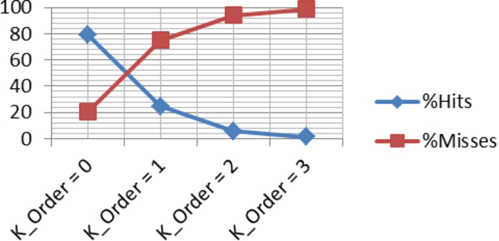
Why do Markov chains based algorithms perform so poorly in these experiments? Fig. 9 shows, the PPM statistics for the experiments run with 5 users with results shown in Table 5. The percentage of hits and misses were computed for all K orders across all users. The PPM algorithm starts at the highest K order ( $K = 3$ ) and each time the context (input) of size K of the input is not matched the algorithm scales down to a lower K order (matches a shorter portion of the input). Figure 9 shows that the PPM algorithm operates at K order = 0 about 80% of the time. This means that 80% of the time the PPM algorithm fails to match its input, applies a penalty to the path probability for the input and moves down to a lower K order Markov graph until it reaches K order = 0. This explains the poor performance of PPM and other higher K order algorithms (3rd Order MC, All-K) and also explains why higher order Markov chain algorithms have accuracy performance recall output values similar to lower order Markov chain algorithms.

Fig. 9.

PPM matches and miss matches per K order = 3 (E₁).

Accuracy reported by HTM algorithms scales better with increasing number of users and web destinations than the accuracy reported by alternate Markov chains based algorithms as shown in Table 6. Table 6 shows the difference in recall accuracy between experiments (E₁, Table 21, Appendix H) run for 5 and 100 users, with different number of visited web destination (1000, 5000, 10,000), over 5 train days and 1 test day using synthetic data. The high and low recall values of all HTM algorithms and alternate algorithms were recorded and the difference between accuracy values for 5 and 100 users was tabulated. Table 6 shows that HTM algorithms scale better (smaller differences) than alternate algorithms with a maximum of 13% loss in accuracy when tracking 1000 web destinations moving from 5 to 100 users compared to 41% loss in accuracy for alternate MC based algorithms running equivalent experiments. For 5000 and 10,000 web destinations, the scale factor for the HTM algorithm improves even more and is as low as 1% for high recall values.

Table 6

Recall accuracy scaling from 5 up to 100 users for 5 train days and 1 test day (E₁)

Number of destinations	Scale factor based on recall differences from 5 to 100 users

	HTM high recall difference	HTM low recall difference	Alternate algorithm high recall difference	Alternate algorithm low recall difference
1000 destinations	0.13	0.05	0.407	0.342
5000 destinations	0.01	0.1	0.41	0.35
10,000 destinations	0.01	0.06	0.41	0.41

To further understand how accuracy is specifically impacted by the number of destinations in the data set, it was observed that synthetic data accuracy performance increases substantially (E₁, Table 21, Appendix H) as number of destinations increases from 1000 to 5000 (from 54% recall accuracy to 99% for 500 users with 5 days of train data and 3 observations of test data), minimally from 5000 to 10,000. Synthetic data accuracy scalability measured for increasing number of users with 5000 web destinations visited (E₅) is high for the top 2 best performing HTM algorithms (BottomUp at layer 1 and TopTop) consistently at 99% recall accuracy for 150, 250 350, 450, 500 users (see Fig. 10).

Fig. 10.

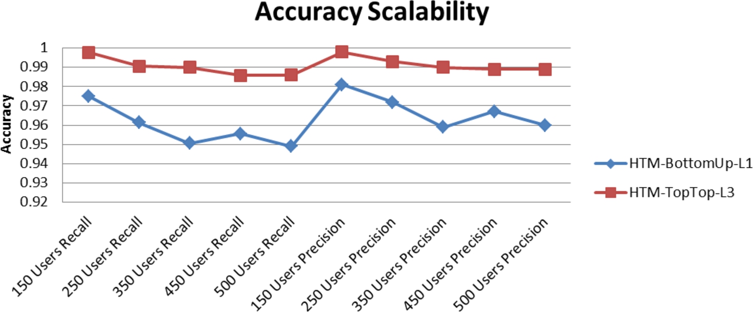
Accuracy scalability synthetic data, 5 train and 1 test days (E₅).

The weighted sum based HTM algorithms (BottomUp at layers 1 and 3 and TopTop) outperformed all other HTM algorithms. To understand why, let us compare the average based algorithm to the weighted sum based algorithm. Consider an observation of size 5 (5 web sites visited) where the input received by the HTM is $⟨ 1, 2, 3, 4, 5 ⟩$ which matches 100% of the learned input as 5 distinct nodes (5 sequences each of size 1). That is, for the average HTM algorithm $FFB = (1 + 1 + 1 + 1 + 1) / 5 = 1.0$ (100%). Now consider the calculation (as done for the BottomUp algorithm) for the average weighted sum proportional to the matched input $FFB = [(1 / 5) + (1 / 5) + (1 / 5) + (1 / 5) + (1 / 5)] / 5 = 1 / 5$ (20%). Now assume a new input $⟨ 1, 2, 3, 4, 5 ⟩$ which matches 100% of the learned input as a single sequence of 5 nodes (1 sequence of size 5). In this case, using the average algorithm $FFB = 1 / 1 = 1$ (100%), while using the average weighted sum algorithm $FFB = [5 / 5] / 1 = 1$ (100%). The average algorithm produces the same recall accuracy whether an entire sequence is matched or only individual elements of the sequence are matched, while weighted sum based algorithms give more weight to longer sequences over shorter ones increasing the discriminating power of the solution.

In order to verify the ability of the HTM to handle noise, several experiments were conducted. Experiments (E₂) using synthetic data with simulated concept drift via “Random Walk” show a reduction in accuracy of up to 25%, indicating that the HTM is susceptible to random splitting of learned sequences. Concept drift which adds new connections at the end of learned sequences reduces accuracy only by up to 11%. Experiments which simulated DOS attacks (E₃) run across all HTM algorithms with synthetic data reduced accuracy by up to 11%, while experiments which simulated Phish attacks (E₄) reduced accuracy only by up to 5%.

5.2. Results using real network data sets

Experiments were also conducted with real network data collected over a period of a month from a cellular data network. Train data sets ranged from 5 to 10 days and 1, 2, 3 test days. Results, at first were modest (E₉). For instance, for 5 users with 5 days’ worth of train data and 2 days’ worth of test data produced results with recall accuracy as high as 81% for HTM algorithms and 10% for Markov chains based algorithms. Visual observation of this data set showed a high recurrence of repeating continuous patterns of a single destination (e.g. 48, 48, 48, 48) within observations compared to similar measurements for synthetic data. This was confirmed by intra-observation repetitiveness (IOR) measurements which for some users were as high as 94%, indicating that within a user observation on average there were 47 repeating destinations out of 50. Calibration of real network data run against the HTM also showed poor performance with the best HTM algorithms (BottomUp and TopTop) scoring recall accuracy values (for experiments E₉ with 5 users, 5 train and 2 test days’ worth of data) ranging from 71% to 100%. Unexpectedly, alternate Markov chain algorithms in calibration tests with the same data set performed very well with the lowest recall accuracy value of 99%. It appears that alternate Markov chain based algorithms perform well when test and train data are very similar but when the data set differ as in the user identification experiments (E₆) then recall accuracy scores do not go above 10%.

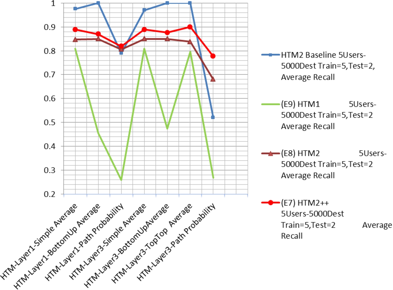
The HTM was modified (version 2 HTM2++) in the implementation of the sequence termination condition (TC₃) of the HTM spatial and temporal poolers to account for continuous repeated destinations. The same set of experiments was repeated (E₇) but this time any repeated destinations that occurred at the exact same time were removed from the real network dataset. The reduction was applied to all train and test data files and accounted for a total reduction in repeated destinations of about 35%. The IOR values decreased and recall accuracy increased. For instance, with real network data for 10 users with 5 train days and 1 test day, IOR decreased by 7% and 9% for train and test data sets respectively while recall accuracy increased by 8% with the recall accuracy values shown in Table 7.

Table 7
Real cellular network data recall accuracy results (E₇)

Train/test days Recall results from real cellular network using HTM algorithms

5 users high recall 10 users high recall 5 users low recall 10 users low recall

5 train, 1 test days 0.95 0.87 0.75 0.64

5 train, 2 test days 0.90 0.79 0.78 0.61

10 train, 3 test days 0.86 0.81 0.72 0.64

Train/test days	Recall results from real cellular network using HTM algorithms
5 train, 1 test days	0.95	0.87	0.75	0.64
5 train, 2 test days	0.90	0.79	0.78	0.61
10 train, 3 test days	0.86	0.81	0.72	0.64

To determine if results using 10 users with real network data had statistical significance we took the experiment from Table 7 using real network data for 10 users for 5 train days and 1 test day. This experiment produced a “high” recall accuracy value of 87% (86.7). We repeated the same experiment 30 times, skipping the first 5, 10, 15, 20, …up to 150 destinations for each experiment. This mimics starting an experiment at a different place in the real data stream. The value of α chosen was 0.01, the research hypothesis was that the recall accuracy over these experiments was greater than 85.8%. The calculated sample standard deviation was 0.0084, the standard error mean was 0.0015, and the mean was 0.8625, while the z-score was 2.92. These results are significant at the 0.0018 level.

Fig. 11.

Accuracy comparisons of all HTM versions (E₇, E₈, E₉) including removal of same time destinations.

Why was HTM1 (the original version of the HTM) unable to recognize repetitive continuous patterns? HTM1 broke up repetitive patterns instead of treating them as sequences. So pattern, 1, 2, 3, 1, 2, 3, 1, 2, 3 was seen as pattern 1, 2, 3 occurring 3 times (which is good), but sequence 2, 2, 2, 2, 2, 2, 2, 2 was seen as a single destination 2 visited 8 times. This means that a user who seldom visits destination 2 and another who visits it in a sequence will produce analogous similarity statistics since for a single repeating continuous destination, HTM1 does not see a sequence of destinations but only a single element. HTM version 2 (HTM2) modifies terminating condition TC₃ to continue to process repeated destinations already in the sequence until a new destination not already in the sequence is encountered or terminating conditions TC₁ or TC₂ are met. In order to understand the recall accuracy improvements between experiments E₉, E₈, and E₇, Fig. 11 shows the results for user identification tests run with 5 users with 5 train and 2 test days’ worth of real data. HTM1 represents version 1 of the HTMs without the fix to address continuous repetitive patterns (E₉), HTM2 is the second version of the HTM which addresses repetitive continuous patterns but is run on the same real data set as HTM1 (E₈). HTM2++ is HTM2 run on the real data set where web destinations repeated at the exact same time are removed from the input (E₇). The baseline in Fig. 11 is based on running the experiments on the equivalent synthetic data set. The association of higher levels of IOR measurements with the inferior accuracy results was further investigated and experiments were run (beyond experiments reported in Table 3) with the same data set for 10 users (5 train days/1 test day), this time completely eliminating repeating continuous patterns of a single destination within observations in the input to determine if this would further positively impact accuracy results. While IOR continued to decrease (additional 8% for both train and test data sets), unexpectedly, accuracy never improved beyond 87%.

While investigating these results further, the real network data set was run through an algorithm that computed and thus measured concept drift by converting the concept drift generator for synthetic data to a concept drift detector for real network data. This concept drift detector identified changed user behavior in the test data set due to visits to new connections among existing nodes ( ${CD}_{e}$ ) and new connections to new nodes ( ${CD}_{n}$ ) as shown in Table 8.

Table 8

Concept drift measured in real cellular network data (E₇)

Train/test days	Concept drift (CD) from real network data

	5 users CD_e existing connections	10 users CD_e existing connections	5 users CD_n new connections	10 users CD_n new connections
5 train, 1 test days	0.19	0.20	0.05	0.07
5 train, 2 test days	0.20	0.21	0.07	0.09
10 train, 3 test days	0.18	0.19	0.07	0.08

The average ${CD}_{e}$ concept drift is 20% and ${CD}_{n}$ is 7% which is very similar to the simulated concept drift levels used for synthetic data. In order to determine the impact of concept drift on recall accuracy for real network data experiments, the HTM prototype was further modified to continuously learn during inference (E₁₃). Preliminary results, using only the BottomUp approach run at HTM layer 3, show that recall accuracy improves with the real network data for 5, 10 users for 5 train days and 1, 2, 3 test days. Specifically, recall accuracy for 5 users improved on average 4% and 2% for continuous baseline and continuous inference respectively and 6% and 1% respectively for 10 users. Table 9 shows details of these results.

Table 9

Recall accuracy when continuous learning is applied to real network data (E₁₃)

Train/test days	Continuous learning (BottomUp layer 3) recall results from real cellular network

	5 users recall continuous baseline/normal	10 users recall continuous baseline/normal	5 users recall continuous inference/normal	10 users recall continuous inference/normal
5 train, 1 test days	0.983/0.95	0.931/0.87	0.983/0.95	0.899/0.87
5 train, 2 test days	0.88/0.876	0.847/0.788	0.868/0.876	0.776/0.788
10 train, 3 test days	0.847/0.773	0.826/0.764	0.807/0.773	0.766/0.764

Experiments with real network data which simulated DOS attacks (E₁₀) run across all HTM algorithms reduced accuracy by up to 8% while experiments which simulated Phish attacks (E₁₁) reduced accuracy only by up to 4%. Figure 12 shows the results of (E₁₄) using continuous learning to mitigate the user attribution effects under a DOS attack. The baseline, “normal” in Fig. 12, represents experiments run without continuous learning. The results show that when a subset of users (four out of ten) is under attack during the inference phase, it is possible to get improved attribution recognition accuracy (even over scenarios where no attacks are present) when the HTM algorithm can learn perfectly (continuous baseline). On the other hand, using inference to select which sequences to learn during continuous learning (continuous inference) produces mixed results. DOS attacks conducted during the inference phase produce decreased recognition accuracy performance when continuous inference learning is enabled possibly due to the fact that attacked sites were already learned by this user before the attack took place and do not create new distinctive patterns. Phish attacks instead produced better recognition accuracy performance possibly due to the fact that attacked sites were new and not learned until after the attack making it easier to infer them correctly.

Fig. 12.

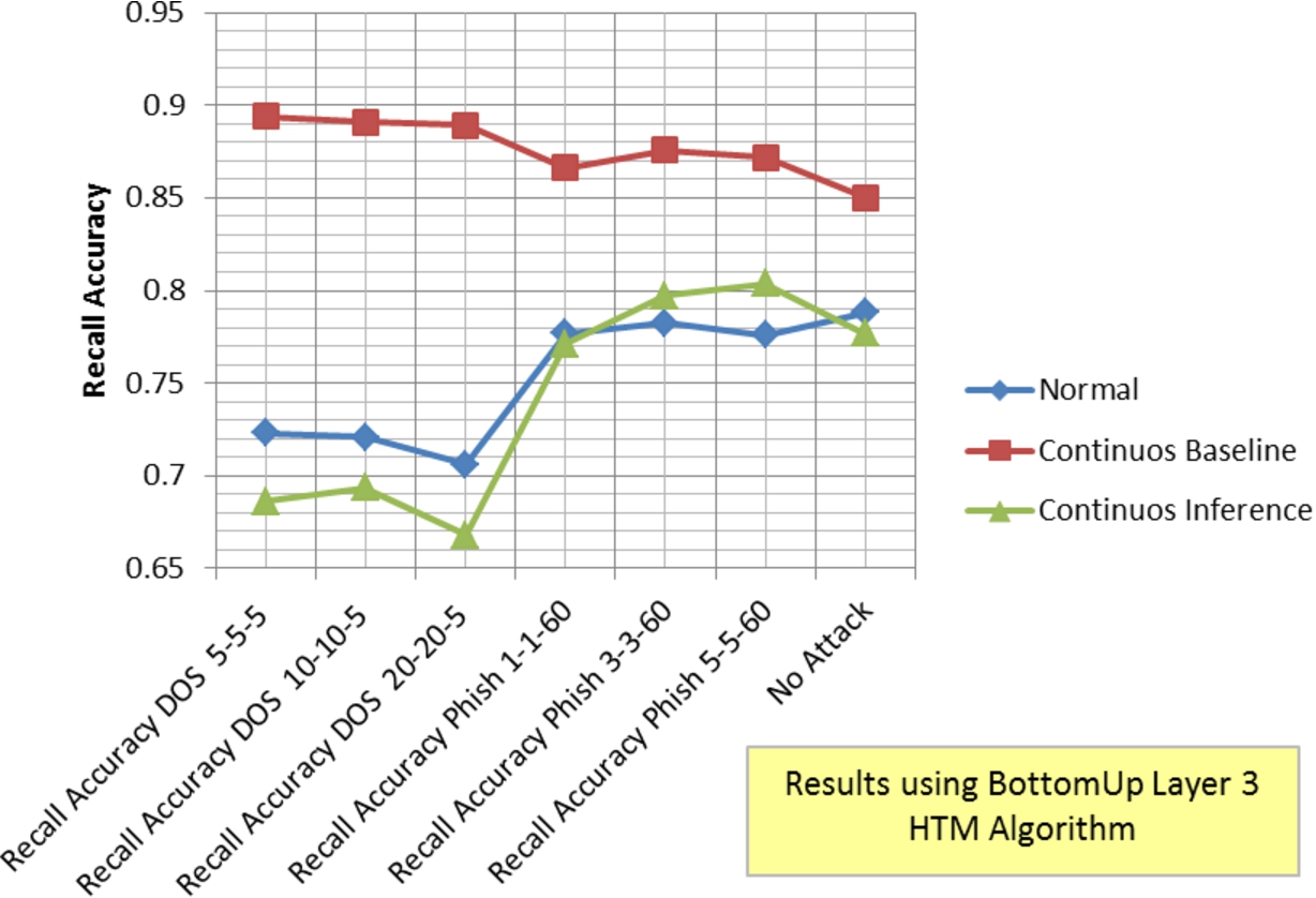
Recall accuracy using continuous learning during DOS and Phish attacks (E₁₄).

5.3. Session identification experiment results

The motivation for conducting session identification experiments is to determine how much different session identification approaches applied during HTM training impact the ability of the HTM to infer accurately (when used under conditions that emulate real life scenarios specific to each session identification algorithm).

Session identification experiment results showed that the sliding window session identification algorithm (which operates normally with some level of randomness) when measured against “perfect” tracking algorithms such as source IP address and TCP timestamp (that are exposed to simulated real life conditions which introduce noise in the data set) can outperform both of these algorithms. The average recall accuracy for all experiments across 5 and 10 users is shown in Fig. 13. To put things in perspective, a window size of 1 min, produced a change in the original train data set (loss of web destinations) of 57%, yet recall accuracy during inference is reported at 92% (Sliding Window worst result), compared to the best performing TCP timestamp (with 10% data loss and 10% device resets) which reports average recall accuracy value of 83%. These results warrant further study into the impact of noise on the session identification algorithms presented in this study.

Fig. 13.

Aggregate session identification recall accuracy results.

6. Security and privacy considerations

This study addresses the important problem of user attribution leveraging communication traffic. A relevant property of user attribution as implemented in this study is that it is privacy preserving with respect to the real identity of the user. Consider the following real-world scenario where the user attribution solution described in this paper is deployed in an access network (possibly a cellular/WIFI operator network or at Internet points of presence) and monitors HTTP traffic. As traffic passes through the user attribution solution (UAS) as proposed in this paper, the solution learns to recognize users (User 1, User 2, User 3, …, User N) based on each user’s past communication behavior. After the learning stage, the UAS can recognize users (inference stage) based on learned communication patterns when users re-enter the network possibly using a new source IP address and new authorization credentials without knowing the user specific identity (User 1 is Joe Smith). In the context of security, accuracy and the (minimal) amount of test data used by HTM algorithms to recognize users are the key measures of success for the UAS. The majority of experiments conducted in this study measured recall accuracy; in addition, experiments conducted which leveraged just 3 observations in the test data sets provide good insights on how quickly the user attribution solution proposed in this study could recognize users.

There are several applications in the area of security that benefit from being able to address the user attribution problem. Specifically, in the area of intrusion detection, the HTM-based approach used to identify users can be used before, during or after an attack has taken place to identify the communication traffic associated with the user that needs to be stopped or rate limited.

The “user attribution problem” is generic and not tied to attack scenarios, but it can still be used to recognize and stop malicious users. Consider a second real-world scenario where the UAS is coupled with an intrusion detection and prevention system (IDPS) so that both receive the same communication input but instead of using the source IP address to recognize users (due to the unreliability of this source), the IDPS uses the user labels (User 1, User 2, User 3, …, User N) associated with the given input provided by the UAS. The UAS after it has completed the training phase and it has entered the inference phase provides user labels to the IDPS. Assume the IDPS (out of scope for this study) detects anomalous behavior with communication traffic belonging to User 4 and blocks all HTTP traffic associated with this user label. User 4, unable to access the Internet decides to re-enter the network next day from a different location, possibly using a different access network (e.g. WIFI access point instead of a cellular network). User 4 likely using a brand new assigned IP address is able to access the Internet, until the UAS recognizes User 4 and passes this user label to the IDPS which will again block this user before the user can start to perform malicious activities.

The experiments run in this study show that it is possible to recognize communication traffic as belonging to a given user even during DOS or phish attacks originating from mobile devices albeit less effectively. We are not aware of reported DOS attacks that originate from mobile devices. Operators do report DOS attacks such as DNS amplification attacks originating from the Internet destined for IP addresses of mobile devices. Such attacks are typically stopped by operators using firewalls deployed at Internet peering points and do not impact user attribution as defined in this study, since they do not originate from mobile devices. Analysis of DOS attack traces made available by the operator where real network data was collected show the typical DOS attack pattern of extremely high volume of messages, sent within extremely tight time windows to the same destination IP address. If such attack patterns were to originate from many mobile devices then the UAS could easily filter them out (same destinations within the same time stamp) as was done in experiments E₇.

What if after an attack occurred, traces of the communication traffic of many users were analyzed to tie that traffic to a possible physical human? The UAS could be trained to recognize communication traffic for users and bind those users to real humans (User 4 is Joe Smith). Like previous examples, the UAS relies on inference to attribute communication traffic to a given user and thus it suffers from possible false negative or false positive errors as opposed to a typical authentication system which relies on fixed tokens like secret key/passwords/cookies. However, it is highly unlikely that such tokens are present in the communication traffic collected from communication logs/traces for user traffic destined to specific web destinations. Even if present, these security tokens have meaning only to the end systems that issued them. Because of these reasons the HTM-based approach proposed in this study could be used to address network forensic investigations.

What if the described scenarios of intrusion detection and network forensic could only have access to encrypted user traffic data? Would the HTM-based approach still be able to recognize user communication traffic? Consider the following three different scenarios: (1) user communication to a secure network server via IPSEC, (2) user communication to a web server supporting a secure HTTPS connection, (3) user leveraging the anonymizing Tor network [16] to communicate with a web server. The answer to the above questions depend on whether the destination IP address in the encrypted communication traffic received by the attribution system represents the actual destination that the user intended to visit. This is possible with IPSEC since the IPSEC tunnel could terminate at the site being visited, it is likely with HTTPS since the secure connection terminates at the server being visited, but impossible with Tor destined traffic since Tor encrypts the original data, including the destination IP address, several times and sends it through a virtual circuit comprising successive, randomly selected Tor relays.

What if a strategic attacker, who knows about the attribution system being in place, takes actions to avoid it? The attribution system monitors normal traffic and not malicious traffic, assuming that the original user has possession of the compromised device, then that user would continue to use the device normally, with normal “concept drift” over time, plus the background malicious activity. In this case the attribution system has a good chance of recognizing the user. However, if the malicious activity completely takes over the device (possibly the device is stolen) then the new malicious user will have different user behavior and this malicious user would not be recognized by the attribution system.

Another security application where user attribution as addressed in this study could be leveraged is in the area of user communication traffic identification under source spoofing conditions. Assume that spoofing or impersonation could take place as two users call or message each other. In this case, the sequence of destinations (numbers called or messaged to) originating from a potential impersonator are run against HTMs which are trained with sequences of destinations accessed by valid users. These sequences would be identified as being spoofed if the HTM inferred user (associated with these learned sequences) does not match the reported originating user. For instance, assume that for Voice over IP (VOIP) scenarios the HTM at train time monitors SIP INVITE messages which identify calls originating from User 1. At train time the HTM learns that User 1 calls $⟨ User 2, User 5, User 8 ⟩$ in that order. Assume that User 1 is being impersonated and the impersonating User 1 calls $⟨ User 5, User 8, User 2 ⟩$ , then this call pattern is not likely to match User 1 (the reported originating user in the SIP INVITE message) call patterns and thus User 1 would be identified as a possible impersonator. Note that even if the impersonator were to guess the right sequence order of users to call, it is not guaranteed that the HTM would be fooled into identifying the impersonating User 1 as the authentic User 1. This is because the HTM learns the inter destination arrival rate TC₂ for all learned sequences. This means that if the HTM learned the following sequence $⟨ User 2, User 5, User 8 ⟩$ for User 1 and for another User 4 it learned sequence $⟨ User 5, User 8 ⟩$ , then the impersonating User 1 could call the same users as the original User 1 but with different inter arrival times so that two sequences could be generated: $⟨ User 2 ⟩$ , $⟨ User 5, User 8 ⟩$ . In this case User 4, different from the originating User 1 reported in the SIP INVITE message, would be identified as matching the input sequences and User 1 would again be identified as an impersonator. Session identification, however, would likely leverage a different identification approach for the VOIP scenarios than what has been proposed in this study. Assuming that the train data set is trusted, the originating user is identified in the SIP INVITE message (“FROM/Contact” SIP headers) and this tracking header can be used to create user sessions, instead of using the TCP timestamps. This session identification approach works especially well when SIP INVITE messages ride over the UDP protocol which cannot use the TCP timestamp.

7. Limitations

The following sections describe implementation constraints faced during the experimentation phase as well as envisioned challenges faced using the TCP timestamp approach.

7.1. Limitations in implementation

The HTM prototype was completely written in Java. The performance scalability of HTMs measured in terms of run-time and space (memory needed at run-time) was a challenge in this study which limited the experiments to a maximum of 500 users. All experiments were executed on a Quad i7-3820QM 2.7–3.7 GHz with 16 GB RAM laptop. Threading (one thread per HTM) and caching (of already computed results derived by performing inference traversal of the Markov chains within each layer of the HTM) were two techniques that considerably improved the inference performance of the HTM allowing completing the experiments for 500 users in reasonable times. When first implemented threads improved run-time performance by almost 100% so that running the HTM algorithms for 2 users would take about 30 min to complete in single threaded mode but using multiple threads the experiment would complete in 16 min. By adding caching of results of Markov chain searches, performance dropped from 16 min to 6 min for the same set of experiments. Further optimizations in how threads were used (limiting the number of concurrent threads to 8) and other enhancements in the cache algorithms to maximize cache hits and minimize collisions resulted in run times of 16 min to 1 h and 15 min for 5 to 100 users using 5 days’ worth of synthetic train data and 1 day worth of test data and 7 min to 5 h for 5 to 500 users for 5000 destinations using 5 days’ worth of synthetic train data and 3 observations worth of test data. In contrast, the highest run time for alternate Markov chain based algorithms was 3 min for equivalent tests which involved 500 users. Alternate Markov chains algorithms have much better run times since discovery of the start of the input sequence is determined in constant time and matching of the sequence against the “context” occurs in time proportional to the size of the input since all alternate Markov chain algorithms are based on extensions of a 1st order Markov graph which matches the input completely based on the on the very first web destination in the sequence. HTM algorithms on the other hand have search run times that are proportional to the size of the entire input (all sequences) learned at training time as well as the size of the input sequence since HTMs perform an exhaustive search of all Markov chains at each HTM layer.

The amount of runtime memory needed by HTMs also proved to be a limiting factor in being able to extend experiments beyond 500 users. The HTM was run with a JVM setting of 14 GB of RAM but a limiting factor of the HTM design is the need for the Max HTM Output Layer (as shown in Fig. 8) to receive and hold one observation’s worth of feed forward beliefs from each HTM before being able to decide which HTM has the “best” feed forward belief. Increasing the number of users increases the number of HTMs which also increases the amount of RAM main memory needed to run the experiment. When the Java JVM starts to run out of the allocated RAM memory and starts to use hard drive virtual memory, run-time performance deteriorates dramatically eventually preventing forward progress.

7.2. Limitations in approach

There are a few limitations tied to the use of TCP timestamps as a communication session identification algorithm. In this study, the TCP timestamp session identification is used in two situations. The first occurs during training of an HTM when session identification is used to identify up to 50 observations as belonging to a given source associated with a specific HTM representing a given user. The second occurs during inference when session identification is used to create anonymous sessions for each observation which are distributed to all HTMs so that each HTM can perform inference on the observation to determine how well the observation matches learned input for each HTM. During the training phase the following scenarios are not allowed as they will corrupt the training data set:

A single user leveraging multiple devices.

Many users sharing the same device.

The user recycling the device.

A single user using multiple devices at training time would appear as many different sources and thus one HTM would be created for each source. This is a problem because each HTM created at train time identifies a different user when actually training is occurring for only one user. When many users share the same device at train time, the sessions produced are corrupted. These sessions will include data from multiple users and would thus not be representative of any given user. When a user recycles his/her device, the TCP timestamp is reset and this user session will appear as a new source and thus would incorrectly cause a new HTM to be created, thus identifying a new, non-existing user. During the inference phase when anonymous sessions are created only the second scenario is disallowed as the multiple users sharing the same device will create individual sessions with corrupted data belonging to multiple users. During the inference phase a user can use one device to train the HTM and a different device to perform inference. In addition, during inference, when anonymous sessions are created, the device under test can be recycled, as long as partial sessions (containing less than 50 observations) produced because recycling interrupts creation of the previous observation, are discarded. In general, the effect of a recycling device is the restart of a TCP IP connection which resets the TCP timestamp’s TS value. TCP connections are also reset when TCP connections go through middle boxes (Web proxies, NATs, Firewalls, Load Balancers) which split a single TCP connection from device to origin server into two TCP connections; one connection from the device to the middle box and the other from the middle box to the origin server.

If the TCP approach has the reported limitations why was this approach chosen for this study? The TCP timestamp approach provides a reliable way to “track” user communication sessions in a way that is independent of the location or network a device attaches to, thus enabling support for mobility. The authors believe that in real life scenarios, users recycle their mobile devices infrequently, and do not share their personal mobile devices with others. Another practical challenge with the use of TCP timestamp is due to the possibility of loss of tracking accuracy due to clock skew, approaches to address these challenges were presented in Section 3.1.1. A final limitation brought to bear in this study is found in experiments (E₁₄) where DOS attacks during user identification experiments are countered by using “continuous learning”. The results show consistent worse recall accuracy performance when using continuous inference learning. This leads to the observation that continuous learning can improve user identification recall accuracy in the presence of “concept drift” but when presented with repeated continuous patters found in typical DOS attacks, it can perform poorly.

7.3. Further research directions

An assumption made in this study is that users can be identified by learning web sites they visit. An interesting extension of this idea would be to study the user attribution problem in the context of peer-to-peer communication as is the case for messaging and voice calls. A key question would be: Can users be identified based on peer-to-peer patterns of communication? A related question would be: Is the power law at work in peer-to-peer communication scenarios as well? That is, do people tend to communicate (message or call) with a few set of users very often and with many other users infrequently? The security implications of extending the user attribution problem to cover peer-to-peer communication scenarios are especially relevant in the area of detection of spoofing of sources in peer-to-peer communication (e.g. recently RFC 7375 “Secure Telephone Identity Threat Model” has defined voice attacks where the calling party can be impersonated by an attacker).

As mobility will continue to dominate our future and as the Internet of people becomes the Internet of things, the user attribution problem will eventually morph into a device/user attribution problem. It would be interesting to run experiments that utilize all communication traffic originating from a device, not just HTTP traffic, to extend the attribution problem from a user to a source (device/user).

Due to the promising results achieved in this study it is important to extend experiments that seek to improve recall accuracy utilizing a larger real-network data set studying further the impact on user identification accuracy of techniques like continuous learning. The HTM framework will be made available to researchers who wish to extend this work by contacting the authors.

8. Conclusions

The user attribution problem is an old problem that just recently has received the attention of the research community. This problem is very important in the field of security since if one cannot attribute communication traffic to a specific user in a network then one cannot identify the user to determine if that user is performing malicious activities in that network or even more importantly stop/prevent the user from continuing to perform such activity. This is the first study that addresses the user attribution problem in the context of complex networks where mobility is dominant using an extensive set of experiments which used both synthetic and real network data. The approach leveraged behavior based identification using HTMs to extend the research of Herrmann and Yang [24,46]. This research, acknowledges the limitations of traditional tracking identifiers such as cookies and source IP addresses, and introduces TCP timestamps as a new session identification algorithm used to identify communication sessions for mobile users. Results from the experiments conducted in this study are promising. HTMs outperform traditional Markov chains based approaches and can provide high levels of identification accuracy using synthetic data with 99% recall accuracy for up to 500 users and good levels of recall accuracy of 95% and 87% for 5 and 10 users respectively when using cellular network data. Performance was further improved with recall accuracy results of 98% and 90% for 5 and 10 users respectively by implementing continuous learning enabled during inference within HTMs to address the challenge of concept drift found in real cellular networks.

This research has made several contributions in the approach used by extending the hierarchical temporal memory model originally proposed in [19] which was not designed to support sequences and showed that sequence based hierarchical memories can consistently provide higher levels of identification accuracy with higher levels of accuracy scalability than traditional Markov chains. The following represent contributions from this research designed to improve HTM inference accuracy:

This study implements sequence inference using a novel technique which combines traditional variable order Markov chains with the use of longest common subsequence and longest common substring coupled with the persistence of learned sequences to support seven new HTM inference algorithms.

This study introduces the concept of sequence cloning to improve the learning and inference accuracy of Markov chains and of HTMs.

This study introduces the concept of playback to distribute accurately learned sequences from lower to higher layers of the HTM. This reduces learning times and improves inference accuracy in hierarchical models like HTMs.

This study also provides insights into the impact to recall accuracy of the power law distribution at work in complex networks which creates high levels repetition of popular web sites in the data set. The impact to recall accuracy of noise in the data set was studied in the context of simulation of malicious activities and the simulation and observation of context drift in a real network. Experiment results suggest that while partial elimination from the data set of continuous repetition of popular web sites improves accuracy results, complete elimination of such repetition does not produce further improvements. Instead, addressing concept drift found in real networks shows promise as an area of further research for improving attribution accuracy performance.

Footnotes

Example of HTM creation during the training phase

The examples in this section and in Appendix B assume that contiguous repetitive sequences (e.g. $⟨ 48, 48, 48, 48 ⟩$ ) are treated as multiple sequences of size 1 based on terminating condition TC₃ (e.g. $⟨ 48 ⟩$ , $⟨ 48 ⟩$ , $⟨ 48 ⟩$ , $⟨ 48 ⟩$ ) which reflects the implementation in version 1 of the HTM (HTM1 in experiments E₉ found in Table 3).

In order to get a better idea of how beliefs propagate up the HTM network layers, this section of the paper shows what happens during playback of input learned in layer 1 of the HTM as represented in the Markov graph and Markov chains shown in Fig. 14 in Appendix B. Input received at layer 1 by the spatial pooler is organized into sequences with the temporal pooler computing corresponding feed forward beliefs as shown in Table 10. Note that during playback the feed forward belief vector only indicates the matched temporal group (in contrast with the inference phase where feed forward beliefs also record the degree of membership value).

After layer 1 completes initial training, layer 1 starts playback of learned sequences towards layer 2. The spatial pooler at layer 2 maps feed forward beliefs from layer 1 into sequence of coincidences using the sequence termination rules TC_1–3 previously described to combine input into sequences as shown in Table 11.

Having completed initial learning, layer 2 then would convert the received coincidences into the Markov graph and Markov chains as shown below in Fig. 15. Assuming that initial learning is completed at layer 2, layer 2 starts playback in order to train layer 3 as shown in Table 12.

Finally, the spatial pooler at layer 3 converts feed forward beliefs received from layer 2 into sequence of coincidences using the terminating condition rules previously described to combine coincidences into sequences of coincidences as shown in Table 13. Figure 16 shows layer 3 Markov chains.

Examples of HTM inference calculations and FFBs propagation

In order to understand how feed forward beliefs propagate through HTM layers during inference consider the following example. Figure 14 represents Markov chains at layer 1 of the HTM created during the training phase based on the following input sequences (see Table 10 in Appendix A) received in this order during inference: $⟨ S_{1}, S_{2}, S_{3}, S_{4} ⟩$ , $⟨ S_{1}, S_{2}, S_{5} ⟩$ , $⟨ S_{1}, S_{3}, S_{6} ⟩$ , $⟨ S_{1}, S_{3}, S_{6} ⟩$ , $⟨ T_{1}, T_{2}, T_{3} ⟩$ , $⟨ T_{1}, T_{3}, T_{5} ⟩$ , $⟨ T_{6}, T_{5}, T_{7} ⟩$ , $⟨ S_{3}, S_{7}, S_{6}, S_{1} ⟩$ , $⟨ {HL}_{1}, {HL}_{2} ⟩$ , $⟨ {HL}_{1} ⟩$ , $⟨ {HL}_{1}, {HL}_{3} ⟩$ , $⟨ {HL}_{1} ⟩$ , $⟨ {HL}_{1}, {HL}_{2}, {HL}_{3} ⟩$ , $⟨ {UL}_{1}, {UL}_{2}, {UL}_{3}, {UL}_{4} ⟩$ , $⟨ S_{2}, S_{6}, S_{5} ⟩$ , $⟨ S_{1}, S_{6}, S_{8} ⟩$ . These sequences were collected by the spatial pooler based on the sequence terminating conditions TC_1–3 (for this example the max allowed sequence size is 4) previously defined. During the learning phase a single Markov graph is created which is then split into multiple Markov chains based on the algorithm shown in Fig. 6.

Assume that during the inference stage the following input sequences are processed in time order by layer 1 of the HTM: $⟨ S_{1}, S_{3} ⟩$ , $⟨ S_{3}, S_{6} ⟩$ , $⟨ T_{1}, T_{2}, T_{3} ⟩$ , $⟨ T_{6}, T_{9} ⟩$ , $⟨ S_{7}, S_{1} ⟩$ , $⟨ {HL}_{1}, {HL}_{2}, {HL}_{3} ⟩$ , $⟨ {UL}_{1}, {UL}_{2}, {UL}_{4} ⟩$ , $⟨ {UL}_{1}, {UL}_{3} ⟩$ , $⟨ S_{1}, S_{2} ⟩$ , $⟨ S_{1} ⟩$ . Table 14 was created from these inputs based on the FFB calculations from Table 1 applied against the Markov chains in Fig. 14. Also assume that the HTM algorithm used is neither the Path probability nor the BottomUp algorithm.

The calculations below refer to Table 14 as applied at HTM layer 1 to the Markov chains in Fig. 14.

The feed forward beliefs from layer 1 travel to layer 2 as shown in Table 15 below. The mapping of temporal groups $g i$ to coincidences $C_{i}$ was established during the learn phase and is shown in Table 11 in Appendix A. Layer 2 input sequences (coincidences) are created based on terminating conditions TC₁ and TC₃.

The HTM layer 2 input activation level (IAL) calculations from Table 15 are shown below:

Layer 2 of the HTM was created during the training phase (see Table 11 in Appendix A) and is shown below.

The feed forward beliefs generated at layer 2 to be sent to layer 3 are computed as shown in Table 16.

Table 16 was created based on the following calculations applied against the Markov chains in Fig. 15:

Layer 3 of the HTM was created during the training phase and is shown below.

The feed forward beliefs from layer 2 travel to layer 3 as shown in the Table 17. The mapping of temporal groups $g j$ to coincidences $C_{j}$ was established during the training phase and is shown in Table 13 in Appendix A.

The HTM layer 3 input activation level (IAL) calculations from Table 17 are shown below:

The feed forward beliefs generated at layer 3 to be sent to the Max Output layer are computed as shown below.

The calculations below belong to Table 18 based on the Makov chains of HTM layer 3 in Fig. 16.

$IS = ⟨ C_{1}, C_{2}, C_{3} ⟩$ then $LLS = ⟨ C_{1}, C_{2} ⟩$ and $⟨ C_{2}, C_{3} ⟩$ since $DM (C_{1}, C_{2}) = DM (C_{2}, C_{3})$ and $SP (C_{1}, C_{2}) = SP (C_{2}, C_{3})$ , $SS = (2 / 3 \times 0.495) + (2 / 3 \times 0.495) = 0.66$ , $SP = (1 / 10 \times 0.01)$ , $DM = (SS, SP) = 0.66$ , $λ_{Output} = FFB \times IAL = min (1, 0.661) \times 0.737 = 0.49$ .

$IS = ⟨ C_{3}, C_{2} ⟩$ then $LLS = ⟨ C_{2} ⟩$ since $DM (C_{2}) = DM (C_{1}, C_{2}) = DM (C_{2}, C_{3})$ and $SP (C_{2}) > SP (C 1, C_{2})$ and $SP (C_{2}, C_{3})$ , $SS = (1 / 2 \times 0.495) + (1 / 2 \times 0.495) = 0.495$ , $SP = (2 / 10 \times 0.01)$ , $DM = (SS, SP) = 0.495$ , $λ_{Output} = FFB \times IAL = min (1, 0.497) \times 0.715 = 0.355$ .

At layer 3 $λ_{Output}$ is sent directly to the Max Output layer, but for layers 1 and 2 the matched Markov chain is used as an index into vectors $λ_{2}$ and $λ_{3}$ . Since it is possible to match more than one Markov chain as shown for input sequence $⟨ C_{1}, C_{2}, C_{3} ⟩$ the single chosen Markov chain is non-deterministic (HTM implementation dependent).

Example of longest common subsequence computation

Consider the following examples to illustrate the use of Eqs (1) ${LCS}_{m}$ and (2) ${LCSU}_{m}$

The best match is achieved with example (1) since all of the input sequence is matched against the learned sequence. The next best match is example (3) which matches all of the input but not from the beginning of the learned sequence. The worst match is example (2) which matches part of the input, albeit from the beginning of the learned sequence.

Computing Path Probability

Assume that each element of sequence LLS has its path probability computed according to Eqs (11), (12) and probability values stored in table Learned_LLS_Nodes, as shown in Fig. 17. Then ComputePathProbability computes the path probability of $IS$ based on sequence LLS as shown in Fig. 17.

For instance, assume $IS = ⟨ S_{1}, S_{3}, S_{4} ⟩$ then from Fig. 14 $LLS = ⟨ S_{1}, S_{3}, S_{6} ⟩$ then $\begin{array}{l} P ({LLS}_{1}) = P ({LLS}_{start \to S_{1}}) = 4 / 16 since {LLS}_{1} = = {IS}_{1} from (11), \\ P ({LLS}_{2}) = P ({LLS}_{S_{1} \to S_{3}}) = P ({LLS}_{2} | {LLS}_{1}) = 2 / 4 \\ since {LLS}_{2} = = {IS}_{2} from condition (12.a), \\ P ({LLS}_{3}) = penalty = 0.0001 since {LLS}_{3} \neq {IS}_{3} from condition (12.b), \\ P (LLS) = 4 / 16 \times 2 / 4 \times 0.0001 . \end{array}$

Another example consider $IS = ⟨ S_{1}, S_{4} ⟩$ and assume that $LLS = ⟨ S_{1}, S_{2}, S_{3}, S_{4} ⟩$ then $\begin{array}{l} P ({LLS}_{1}) = P ({LLS}_{start \to S_{1}}) = 4 / 16 since {LLS}_{1} = = {IS}_{1} from (11), \\ P ({LLS}_{2}) = P ({LLS}_{3}) = penalty = (0.0001 \times 2) \\ since {IS}_{2} = = {LLS}_{4} from condition (12.c), \\ P (LLS) = 4 / 16 \times (0.0001 \times 2) . \end{array}$

Another example consider $IS = ⟨ H_{1}, H_{4}, H_{5}, H_{2} ⟩$ then from Fig. 14 $LLS = ⟨ H_{1}, H_{2} ⟩$ then $\begin{array}{l} P ({LLS}_{1}) = P ({LLS}_{start \to H_{1}}) = 5 / 16 since {LSS}_{1} = = {IS}_{1} from (11), \\ P ({LLS}_{2}) = penalty = 0.0001 since {IS}_{2} \neq {LLS}_{2} from condition (12.b), \\ P ({LLS}_{3}) = penalty = 0.0001 since {IS}_{3} \neq {LLS}_{2} from condition (12.b), \\ P ({LLS}_{4}) = P ({LLS}_{H_{1} \to H_{2}}) = 2 / 5 since {IS}_{4} = = {LLS}_{2} from condition (12.a), \\ P (LLS) = 4 / 16 \times 0.0001 \times 0.0001 \times 2 / 5 . \end{array}$

The first example produces the best match. The second example produces the second best match and the third example the worst match. Compare these results to utilization of longest common sequence and longest common substring calculations and the results are different. When using equations feed forward belief calculations 1 and 2, the second example produces the best match while the first example produces the second best result and the third example produces the worst result. Equations (1) and (2) reward matching all elements of the input sequence $IS$ , whereas the probability based computations are more sensitive to any mismatch between input and learned sequence. Another way to look at it, is that longest common based algorithms of similarity match the input more “loosely” than probability based algorithms.

Understanding HTM algorithms

To understand how HTM algorithms work consider the following example where input to the Max Output Layer is generated during inference for two HTMs ( ${HTM}_{A}$ , ${HTM}_{B}$ , see Table 19) from the same observation (made up of several input sequences totaling 50 web destinations).

For this example, for all HTM algorithms, the observation matches sequences learned by ${HTM}_{B}$ better than sequences learned by ${HTM}_{A}$ since ${HTM}_{B} = {max}_{{HTM}_{A, B}} (Average ()) = {max}_{{HTM}_{A, B}} (Weighted Sum ()) = {max}_{{HTM}_{A, B}} (Path Probability ())$ (see Eq. (17)).

The design of synthetic data

Synthetic train and test data was produced for both the HTM and Markov chain (MC) based algorithms. The User Attribution solution was verified against synthetic data that mimics user web visits found in real world scenarios as shown in Fig. 18, using the algorithm presented in Fig. 19. The User Attribution solution was also verified against MC approaches. These approaches, as opposed to the HTM, do not leverage any timing information. For Markov chains based approaches tests were performed using the same synthetic data generated by the algorithm in Fig. 19 with the exception that all timing information (time stamp and TS values) was removed so that only sequences of destinations are left to be processed. Training and inference for these alternate approaches took place based on “observations”. Each observation simulated a user web session worth of input and consisted of a predetermined number (50) of web sites visited.

Simulation was performed by using input data that is as representative of real user network traffic as possible. The input to the HTM prototype has the following form: $Timestamp ⟨ TS, Dest ⟩$ , where: (1) Generation of the Timestamp input field was accomplished by modeling devices entering (random distribution arrival times) and leaving (random distribution for service times) the network. (2) Generation of the TCP TS value was accomplished by using a 50/50 ratio of TS values started at a fixed value (iPhones) and random values (Android phones). (3) Generation of destinations (ranked in order of popularity) visited by all users in the simulation follow a power law distribution (Zipf).

Figure 18 shows the input framework within which the simulation was run. A Java application was developed separate from the HTM, which produced, for each user, the synthetic input data as shown in Fig. 18. The data simulated devices associated with users entering the network at random times and initiating multiple communication sessions until the devices are turned off. Table 20 shows the various random parameters that were used in the simulation.

The input generation application creates an input file for each simulated user where the numbers of train and test days are configurable parameters.

The algorithm in Fig. 19 creates 5 simulation days’ worth of synthetic train data for user U_x. This simulation code generates synthetic data for training purposes for both HTM and alternate approaches. Each simulation day contains a random number of user sessions bounded by random intersession times. Each user session for the HTM is made up of a random number of input tokens of the form: $Timestamp ⟨ TS, Dest ⟩$ . Within a user session, the intra session time randomly spaces occurrences of the input tokens. Destinations are selected based on the Zipf distribution, with the most popular destinations having the highest probability of being selected over less popular destinations. The algorithm used to implement the Zipf distribution is based on the Zipf algorithm used in [20]. Next_ZipfRandom in Fig. 19 returns the next web site in rank order from 1 to n (with 1 being the most visited and n the least) following a power law distribution. The algorithm generates web sites that are weight proportional to the Riemann zeta function: $\frac{1^{θ}}{1} + \frac{1^{θ}}{2} + \dots + \frac{1^{θ}}{N}$ . In the algorithm in [20], θ (theta) controls the skewness such that $θ = 1.0$ indicates the highest skew (all nodes have different popularity) and $θ = 0$ indicates the lowest skew (all nodes are equally popular). For this study, theta was set to 0.96.

Test data had to be created using a different approach since it had to be similar to the train data but also maintain a certain level of independence from train data. Three methods were used for generation of synthetic data for the test phase of experiments. All three algorithms (Random Walk, Walk Only and Concept Drift) walk a first order Markov chain of learned destinations which were generated during the training phase of the synthetic data generation process.

In the “Random Walk” the next destination $V_{j}$ , for transitions of the form $V_{i} \to V_{j}$ , is chosen randomly in proportion to the in-degree of the node $V_{j}$ . That is, in proportion to the access frequencies of the neighbors ( $V_{j 1}, \dots, V_{j n}$ ) of the current node ( $V_{i}$ ). If no such neighbor $V_{j}$ exists then the walk proceeds with a new node $V_{i}$ with at least one neighbor, selected from the learned destinations based on a Zipf distribution. Selection of the next destination $V_{j}$ is based on the work of Price [39] who proposed a model of networks formation that gives rise to power-law degree distributions. Price was interested in the power law distribution of citation networks. Specifically, his model showed that a newly appearing paper cites previous ones chosen at random with a probability proportional to the number of citations that those previous papers already have. This property is critical in creating a relationship between train data generated for a given user with test data for that same user. While a relationship must exist between the train and test data sets it must also maintain a certain level of independence between the two sets which is provided by the randomness of the selection of already visited nodes. While the Price model has been applied to simulation of networks traversed by many users, in this study, this model is adjusted to simulate web visits by a single user. As a result the emphasis was not placed exclusively on in-degree or out-degree of network nodes but instead on the frequencies of edges emanating from or terminating to nodes representing web visits to web sites. The algorithm follows with connectivity probability $\begin{matrix} 1 - \frac{O_{i}}{O_{i} + C_{i}} > r (0 ⩽ r ⩽ 1) \end{matrix}$ a learned path proportional to the frequency of the in-degree of web sites along the path. Otherwise it starts a new path. In terms of notation, r is a random number that follows a uniform distribution, $C_{i}$ represents the sum of traversal frequencies of all edges emanating from $V_{i}$ ( $V_{i} \to V_{j 1 - n}$ ) and $O_{i}$ is the out degree of $V_{i}$ . As would happen in real life the algorithm favors learned path patterns, but does also produce variations that simulate “concept drift”. In “Walk Only”, the algorithm selects $V_{j}$ randomly in proportion to access frequencies of all of $V_{i}$ ’s neighbors as long as $V_{i}$ has at least one neighbor. Note that this algorithm minimizes any concept drift since it always follows a learned path as long as one exists, as opposed to the Random Walk algorithm that is constrained by the connectivity probability and the random value of r. In “Context Drift”, the algorithm selects $V_{j}$ using the Walk Only algorithm except for 20% of the $V_{j}$ destinations that are selected as new ones outside of the learned train set. In addition, 10% of the $V_{i} \to V_{j}$ transitions selected during the walk are new (not existing in the train set).

Why use HTMs when dealing with complex networks?

HTMs are unique in stressing the temporal aspect of perception and implementing memory for sequences of patterns that facilitate anticipation. Each level in the hierarchy is trained separately to memorize spatial–temporal objects (patterns) and is able to recognize objects in a bottom-up/top-down process [18]. The HTM hierarchy also enables efficient representation of relationships among many inputs by leveraging reuse of lower level inputs in order to represent higher level concepts at higher levels of the hierarchy. HTMs allow sequence learning (concatenation of spatial and then temporal learning), which provides the ability to make predictions and can be applied to disambiguate input. Only few methods exist that combine spatial and temporal learning in a tight way (e.g. recurrent neural networks can do this a well) [22].

Of specific interest to this study is the evaluation of the distribution of visitors to web sites. Adamic and Huberman [1] studied the distribution of users among web sites by examining usage logs from America Online covering 120,000 sites. They discovered that the distribution of visitors per site follows a universal power law similar to that found by Pareto in income distributions. They reasoned that a small number of sites control the traffic of the web population, a result typical of winner-take-all markets. The authors agree that the World Wide Web gives rise to an asymptotic self-similar structure in which there is no natural scale and the number of users per site is indeed distributed according to a power law. In another study, Adamic and Huberman [2] find inconsistencies in the conclusions of a study by Barabasi and Albert [5] which states that because of preferential treatment, a vertex that acquires more connections than another will increase its connectivity at a higher rate so that the connectivity between nodes increases in line with the growth of the network. This leads to older vertices increasing their connectivity at the expense of younger and leading to the well known “rich-get-richer” phenomenon for highly connected vertices. Adamic and Huberman studied web crawls of 260,000 sites and concluded that all sites are not created equal since no correlation exists between the age of a site and its number of links. They explain that the rate of acquisition of new links varies from site to site and is probably proportional to the number of links the site already has, because the more links the site already has, the more visible it becomes and the more links it will get.

While there has been agreement in the research community that communication traffic has self-similar characteristics, until recently it was believed that complex networks are not invariant or self-similar under large scale transformations. This belief is rooted in the small world property of these networks which would seem to imply that the number of nodes increases exponentially with the diameter of the network rather than following the power law relation expected for self-similar structures. Song, Havlin and Makse [44] analyzed real complex networks, like the web, utilizing a box counting method as a scale invariant renormalization procedure and concluded that, on the contrary, these networks consist of self-repeating patterns on all length scales that suggest they share common self-organizing properties.

What are the implications of addressing the user attribution problem in the context of complex networks? The self-similar, small world and clustering properties together with the preferential attachment characteristic of complex networks supports the notion that users tend to visit a limited number of mostly popular sites with increasing frequencies. How can the approach implemented in this study leverage unique and personal patterns to differentiate among users if different users visit mostly the same sites and this research proposes to use web site visits as a way to uniquely recognize users?

This study has leveraged the power law properties that characterize web traffic of users who visit different web sites. Specifically, the implications of the power law distribution support the notion that while it is true that few web sites get visited very often by all users, many web sites, in the long tail portion of the power law distribution, get visited less often by a variety of users as well. By recording communication patterns of past activity for each user it becomes possible to identify unique and differentiating elements that will enable isolation among users. More specifically, the hypothesis in this study has been that the long tail properties of the distribution of user visits to web sites together with the time order of such visits create conditions for unique differentiation among user patterns that allows to adequately address the user attribution problem.

HTMs have been successfully used in classification problems in a variety of applications such as recognition of USPS handwritten digits [8], speech recognition [17], and prediction of user choices on mobile phones [34]. HTMs have also been used in the area of web analytics which represents an important use case for this study. In a talk given for the Association of Computing Machinery (ACM) in 2009, Subutal Ahmad, vice president of engineering at Numenta, described results of experiments using Numenta’s HTMs to predict user web click behavior for topics and pages of interest to the user. In these experiments web content was partitioned into 177 different topics. In their experiments random prediction reported 0.56% accuracy. By training the HTM with 100,000 user sequences (web pages) and using no temporal context (0th order prediction based on recorded popularity of topics and web pages) the accuracy reported was 23%, which matches what most web sites can do today. By including in the analysis transition probabilities from a given web page to another in the form of 1st order prediction, predictive accuracy increased to 28%. By further leveraging use of variable order prediction, accuracy levels jumped to 45%. Variable order prediction, used in this study, allows prediction to fully leverage the dynamic “context” (different length sequences) of web pages visited by a user.

Tables describing parameters for experiments

Table 25

Experiment types E₇, E₈, E₉, user attribution

Number of users	Number train days/number of test days
5	5/1	5/2	10/3
10	5/1	5/2	10/3

Glossary of HTM abbreviations and symbols

Table 26 provides an explanation for many of the abbreviations, terms and symbols used in HTM computations and algorithms found in Section 3.

References

A.L.

Adamic and

B.A.

Huberman, The nature of markets in the World Wide Web, Quarterly Journal of Electronic Commerce 1 (2000), 5–12.

A.L.

Adamic and

B.A.

Huberman, Power-law distribution of the World Wide Web, Science 287 (2000), 2115.

Baldi,

Frasconi and

Smyth, Modelling the Internet and the Web: Probabilistic Methods and Algorithms, John Wiley & Sons, Chichester, 2003.

Banse,

Herrmann and

Federrath, Tracking users on the Internet with behavioral patterns: Evaluation of its practical feasibility, in: Information Security and Privacy Research, IFIP Advances in Information and Communication Technology, Vol. 376, Springer, Berlin, 2012, pp. 235–248.

A.L.

Barabasi and

Albert, Emergence of scaling in random network, Science 286(5439) (1999), 509–512.

Beacken,

Braun,

D.J.

Imbesi,

L.G.

Greenwald,

M.J.

Geller,

Hartman

M.J.

Chen,

Ter Louw,

Piccirilli and

Bishop LGS’ government communications laboratory and research for the U.S. government, Bell Labs Technical Journal: Vertical Markets 16(3) (2011), 5–28. doi:10.1002/bltj.20519.

Belenky and

Ansari, On IP traceback, IEEE Communications Magazine 41(7) (2003), 142–153.

Bobier, Handwritten digit recognition using hierarchical temporal memory, Unpublished manuscript, Ontario, Canada, 2007, available at: http://arts.uwaterloo.ca/~cnrglab/?q=system/files/SoftComputingFinalProject.pdf.

Burch and

Cheswick, Tracing anonymous packets to their approximate source, in: Lisa’00: Proceedings of the 14th Conference on Systems Administration, USENIX Association, Berkeley, CA, 2000, pp. 319–328.

10.

Casado and

M.J.

Freedman, Peering through the shroud: The effect of edge opacity on IP-based client identification, in: Proceedings of the 4th USENIX/ACM Symposium on Networked Systems Design and Implementation (NSDI), USENIX Association, Berkeley, CA, 2007, pp. 173–186.

11.

H.Y.

Chang,

Narayanan,

S.F.

Wu,

B.M.

Vetter,

Wang,

Brown and

Gong, Deciduous: Decentralized source identification for network-based intrusions, in: Proceedings of the Sixth IFIP/IEEE International Symposium on Integrated Network Management, IEEE Computer Society, 1999, pp. 701–714.

12.

D.D.

Clark and

Landau, Untangling attribution, in: Proceedings of a Workshop on Deterring Cyberattacks: Informing Strategies and Developing Options for U.S. Policy, The National Academies Press, Washington, DC, 2010, pp. 25–40.

13.

Cooley,

Mobasher and

Srivastava, Data preparation for mining World Wide Web browsing patterns, Knowledge and Information Systems 1(1) (1999), 5–32.

14.

G.V.

Cormack and

R.N.S.

Horspool, Data compression using dyanamic Markov modelling, The Computer Journal 30(6) (1987), 541–550.

15.

Deshpande and

Karypis, Selective Markov models for predicting web-page accesses, ACM Transactions on Internet Technology 4(2) (2004), 163–184.

16.

Dingledine,

Mathewson and

Syverson, Tor: The second-generation onion router, in: Proceedings of the 13th USENIX Security Symposium, 2004.

17.

J.V.

Doremalen and

Boves, in: Spoken Digit Recognition Using a Hierarchical Temporal Memory. 9th Annual Conference of the International Speech Communication Association, ISCA, Brisbane, Australia, 2008, pp. 2566–2569.

18.

Duch,

R.J.

Oentaryo and

Pasquier, Cognitive architectures: Where do we go from here?, in: Proceedings of the First Conference on Artificial General Intelligence, IOS Press, Amsterdam, 2008, pp. 122–136.

19.

George and

Widrow, How the brain might work: A hierarchical and temporal model for learning and recognition, Dissertation (Dissertation Abstract International, 69(04), 177; UMI No. 3313576), Stanford University, 2008.

20.

Gray,

Sundaresan,

Engler,

Baclawski and

P.J.

Weinberger, Quickly generating billion-record synthetic databases, in: Proceedings of the 1994 ACM SIGMOD International Conference on Management of Data, Vol. 23, ACM, New York, NY, 1994, pp. 243–252.

21.

Grčar, User profiling: Web usage mining, in: Proceedings of the 7th International Multiconference Information Society, Jožef Stefan Institute, Ljubljana, Slovenia, 2004, pp. 75–78.

22.

Greff, Extending hierarchical temporal memory for sequence classification, Master thesis, Technische Universität Kaiserslautern AG Wissensbasierte Systeme, Saarbrücken, Germany, 2010, available at: http://www.dfki.de/lt/publication_show.php?id=5462.

23.

Hawkins,

George and

Niemasik, Sequence memory for prediction, inference and behavior, Philosophical Transactions of the Royal Society B: Biological Sciences 364(1521) (2009), 1203–1209.

24.

Herrmann,

Banse and

Federrath, Behavior-based tracking: Exploiting characteristic patterns in DNS traffic, Computers & Security 39 (2013), 17–33.

25.

Herrmann,

Gerber,

Banse and

Federrath, Analyzing characteristic host access patterns for re-identification of Web user sessions, in: 15th Nordic Conference on Secure IT Systems (NordSec), Springer, Berlin, 2010, pp. 136–154.

26.

Hill and

Provost, The myth of the double-blind review? Author identification using only citations, SIGKDD Explorations 5 (2003), 179–184.

27.

S.B.

Hill,

D.K.

Agarwal,

Bell and

Volinsky, Building an effective reppresentation for dynamic networks, Journal of Computational and Graphical Statistics 15(3) (2006), 584–608.

28.

Honda,

Nishida,

Raiciu,

Greenhalgh,

Handley and

Tokuda, Is it still possible to extend TCP?, in: ACM/USENIX Internet Measurement Conference (IMC), ACM, New York, NY 2011, pp. 181–194.

29.

Jacobson,

Braden and

Borman, TCP extensions for high performance, Network Working Group Report no. RFC 1323, 1992, available at: The Internet Engineering Task Force (IETF) website.

30.

Kohno,

Broido and

Claffy, Remote physical device fingerprinting, IEEE Transactions on Dependable and Secure Computing 2(2) (2005), 93–108.

31.

Kumar and

P.R.

Raju, A new similarity metric for sequential data, International Journal of Data Wharehousing and Mining 6(4) (2010), 16–32.

32.

Kumpošt and

Matyáš, User profiling and re-identification: Case of university-wide network analysis, in: Proceedings of the 6th International Conference on Trust, Privacy and Security in Digital Business, Springer-Verlag, Berlin, 2009, pp. 1–10.

33.

Liu, Web Data Mining Exploring Hyperlinks, Contents and Usage Data, Springer-Verlag, Berlin, 2008.

34.

W.J.C.

Melis,

Chizuwa and

Kameyama, Evaluation of hierarchical temporal memory for a real world application, in: Fourth International Conference on Innovative Computing, Information and Control, IEEE Computer Society, 2009, pp. 144–147.

35.

Moffat, Implementing the PPM data compression scheme, IEEE Transactions on Communications 38(11) (1990), 1917–1921.

36.

Pearl, Probabilistic Reasoning in Intelligent Systems: Networks of Plausible Inference, 2nd edn, Morgan Kaufmann, San Francisco, CA, 1988, pp. 143–194.

37.

Pitkow, In search for reliable usage data on the WWW, in: Proceedings of the Sixth International WWW Conference, 1997, pp. 451–463.

38.

Pitkow and

Pirolli, Mining longest repeating subsequence to predict World Wide Web surfing, in: Proceedings of USITS’99: The 2nd USENIX Symposium on Internet Technologies & Systems, Vol. 2, USENIX Association, Berkeley, CA, 1999.

39.

D.J. de S.

Price, A general theory of bibliometric and other cumulative advantage processes, Journal of the American Society for Information Science 27(5) (1976), 292–306.

40.

Ravasz and

A.L.

Barabasi, Hierarchical organization in complex networks, Physical Review E 67(2) (2003), 026112.

41.

Rosenstein, What is actually taking place in Web sites: E-commerce lessons from Web server logs, in: ACM Conference on Electronic Commerce, ACM, New York, NY, 2000, pp. 38–43.

42.

Santhanam,

Kumar and

D.P.

Agrawal, Taxonomy of IP traceback, Journal of Information Assurance and Security 1 (2006), 79–94.

43.

Savage,

Wetherall,

Karlin and

Anderson, Practical network support for IP traceback, in: Proceedings of the ACM SIGCOM 2000, ACM, New York, NY, 2001, pp. 295–306.

44.

Song,

Havlin and

H.A.

Makse, Self-similarity of complex networks, Nature 433(7024) (2005), 392–395.

45.

Stone, CenterTrack: An IP overlay network for tracking DoS floods, in: Proceedings of the 9th USENIX Security Symposium, Vol. 9, USENIX Association, Berkeley, CA, 2000.

46.

Yang, Web user behavioral profiling for user identification, Decision Support Systems 49(3) (2010), 261–271.

Train/test days	Recall results from real cellular network using HTM algorithms

	5 users high recall	10 users high recall	5 users low recall	10 users low recall
5 train, 1 test days	0.95	0.87	0.75	0.64
5 train, 2 test days	0.90	0.79	0.78	0.61
10 train, 3 test days	0.86	0.81	0.72	0.64