Using temporal probabilistic logic for optimal monitoring of security events with limited resources

Abstract

Managed security services (MSS) are becoming increasingly popular today. In MSS, enterprises contract a security firm such as Symantec or IBM to manage security of their enterprise network. MSS vendors thus have a small pool of cybersecurity analysts who must monitor many different alerts. In this paper, we study the problem of allocating cybersecurity analysts to alerts generated by intrusion detection systems and other security software. In particular, given an enterprise network (or set of enterprise networks) and information about the value of assets stored at a node (e.g. computer, router) in the network, together with probabilities of compromising a neighbor of a compromised vertex, we show that annotated probabilistic temporal (APT) logic programs allow a defender to express knowledge about the network that captures the probabilities that different nodes will be attacked. In addition, certain APT logic computations, in conjunction with a Stackelberg game theoretic formalization, enable us to capture the attacker’s maximal probability of success as well as his ability to maximize damage. We show how the defender can come up with optimal allocations of tasks to cybersecurity analysts, taking both network information into account as well as a behavioral model of the attacker into account. We show correctness and complexity theorems for both the attacker and the defender. We develop a prototype implementation of three algorithms for the defender that optimize the defender’s objectives and show that these algorithms work well on realistic network sizes.

Keywords

Enterprise systems logic programs computer security behavior modeling

1. Introduction

Managed security services (MSS) are becoming increasingly common today with large enterprises frequently outsourcing security services to a third party. MSS vendors allocate a pool of cybersecurity analysts to “watch over” the networks of their corporate customers. Because security monitoring programs generate lots of alerts, these cybersecurity staff have a heavy burden. The same is true for enterprises who do not use MSSs, but manage security “in-house” (such as government agencies). As enterprise cyber-security tools proliferate, they tend to generate a very large number of alerts [23,64]. In some government and military organizations, the security staff must create a report on each and every alert. Simply put, the time of cybersecurity analysts both within enterprises and in an MSS setting is a scare commodity. An attacker targeting a large enterprise knows that cybersecurity analysts in the targeted company will be swamped with alerts generated by the various security tools installed on the network. He can therefore easily “hide” his attack activity within the large volume of activity within an enterprise network and assume that the false alarms generated by intrusion detection and other cybersecurity software will mask his true positive attacks.

In this paper, we consider an arbitrary MSS which ensures that at any point in time, $k > 0$ security analysts are always watching the alerts (for instance, this is a common guarantee for MSSs). k is not the size of the whole cyber-security staff of the MSS, nor is it even the number of such analysts. For instance, an MSS may always have a team of 16 analysts, each works 6 hour shifts, so that at any given point in time during the day, there are (on average) 4 analysts handling alerts. In this case $k = 4$ .

Like many others, we assume that an enterprise network can be represented as a graph [56]. The vertices of such a graph correspond to networked computers, routers, and anything with an IP address. Some of these vertices may have cyber-security monitoring programs that generate security alerts. For instances, some vertices may have authentication programs [19] that generate alerts when suspicious accesses are made, some vertices may be monitoring DDOS style attacks [53,63], while yet others may perform behavioral analysis to monitor attempts to exfiltrate data [5]. Throughout this paper, we use the term “vertex” to refer to any addressable entity (i.e. with an IP/MAC address) within a network managed by an MSS vendor. As an MSS vendor is securing multiple networks, and as the union of multiple networks is itself a network, we will assume, without loss of generality, that an MSS is providing security services to a single network.

Fig. 1.

Example of graph modeling a computer network where observable vertices are denoted with solid outlines. The source vertices are $v_{1}$ and $v_{2}$ , and the target is $v_{6}$ .

Fig. 2.

Example of a temporal probabilistic k-assignment.

Figure 1 shows a small sample network secured by an MSS. We will explain this example in a formal way in Section 2 but for now, we use it to illustrate the problems addressed in this paper and how they can help improve the security of a network. In the network of Fig. 1, vertices correspond to addressable entities on the network. These hosts could be routers or machines or anything with an IP or MAC address. Some of these vertices are called “source” vertices. These are vertices in the enterprise that the defender believes are attackable by an attacker from outside the enterprise. The defender assigns a value to the assets stored at each vertex in his network. For instance, in Fig. 1, he assigns the value 2 to the assets stored in vertex $v_{5}$ . We will later specify how such assets are valued. In addition, the defender assigns a probability to each edge in the network. For instance, in Fig. 1, the defender assigns a probability of 0.8 to the edge from $v_{1}$ to $v_{3}$ . This specifies the conditional probability (from the defender’s perspective) of vertex $v_{3}$ being compromised by the attacker if he had previously compromised vertex $v_{1}$ . Given such a description of the enterprise network, the defender would like to answer various questions such as those listed below. In the following questions, we assume that we have k security analysts from an MSS team and that each security analyst has a “temporal assignment” schedule telling him, for each time point, which vertices’ security alerts to monitor. Thus, at each time point, such a temporal assignment tells each analyst to watch alerts generate by one vertex. Figure 2 shows 3 such temporal assignments ${ta}_{1}$ , ${ta}_{2}$ and ${ta}_{3}$ when there are $k = 2$ analysts. The first table in this figure ( ${ta}_{1}$ ) tells us that at time 1, two vertices ( $v_{3}$ , $v_{4}$ ) are monitored, while at time 4, $v_{5}$ , $v_{6}$ are monitored. Given such a situation, the results of this paper allow us to answer the following questions.

Given an attack (set of vertices the attacker wishes to target) and an assignment schedule, what is the maximal probability that the attack will succeed Section 4 provides answers to this question.

Given an attack (set of vertices the attacker wishes to target) and an assignment schedule, what is the maximal expected amount of damage (compromised assets) that the attack will cause Section 4 provides answers to this question.

Given a set of k cyber-security analysts, how should the defender create a schedule for them so that the maximal probability in (Q1) above is minimized Section 5 provides answers to this question. In addition, Section 7 suggests “mixed” strategies where the defender can choose one of many possibly temporal assignments in order to further inject uncertainty into the attacker’s mind.

Given a set of k cyber-security analysts, how should the defender create a schedule for them so that the maximal expected damage in (Q2) above is minimized Section 5 provides answers to this question. Section 7 also applies in this case as mentioned above.

The answers to such questions have obvious value to the managed security services vendor in carrying out his job because the answers to (Q3) and (Q4), which the MSS vendor needs, depend on the answers to (Q1) and (Q2) respectively. However, their value goes beyond the act of providing MSSs. Using the methods presented in this paper, the MSS vendor will know that if they increase the number of analysts they use in-house from say k to $k + 1$ or $k + 2$ , then their customers will see a drop in the success probability of attacks the expected damage. This in turn can be used as a selling point to MSS vendors’ customers, leading to increased revenue for the MSS vendor and increased security for the end client.

In order to answer such questions, this paper brings together a mix of 3 major techniques.

Annotated probabilistic temporal (APT) logic to express the network and express the probability of attacks on a vertex, given certain preconditions holding true. We use APT logics for several reasons. First, logic has been used since the time of Aristotle for reasoning about many diverse applications. There is also extensive use of logic in cybersecurity settings [8,12,14–16,24,29]. APT logic programs are used for many things in the paper: first, they are used to express the defender’s knowledge of how an attacker may move through his network over a period of time. They provide a succinct, high-level knowledge representation framework. Second, we reason with APT logics in order to assign analysts to monitor network vertices. The problem of assigning security analysts has both a temporal and a probabilistic dimension. There is a probabilistic dimension because the defender is uncertain about which vertices of the network will be attacked by the attacker. There is a temporal dimension because at each point in time, the defender must allocate security analysts to monitor alerts generated by different hosts (vertices in the network).

Stackelberg game theory (SGT) [7] is used to reason about two things. First, we use SGT in conjunction with APT logic to reason about how the attacker carries out attacks that maximize his probability of success and/or maximize the damage he causes, in accordance with the rules in the APT logic program. By reasoning about the attacker in this way, the MSS vendor can decide how best to come up with a temporal assignment for his k analysts so as to minimize the maximal probability of success and/or the maximal expected damage of the attacker. The reader should note that Stackelberg games have been widely studied and involve only one level of reasoning. The defender reasons about the attacker’s possible actions and strategies and takes actions that optimize some objective based upon the best possible move of the attacker. As a consequence, SGTs are often amenable to integer linear programming (ILP) solutions as opposed to a more complex framework where the defender reasons about the attacker who in turn reasons about the defender and so forth leading to an enormous AI search tree. They have been extensively used in research on securing airports and other physical sites [30,44,51] in place of traditional AI search trees and we follow this trend.

Integer linear programming (ILP) is used to operationally compute the optimal solution for the attacker which either maximizes success probability or maximizes expected damage, and also show how the defender (i.e. the MSS vendor) can optimally create a temporal assignment so that he minimizes either the maximal probability of success or the maximal expected damage of the attacker. There is a long history of using linear programming in probabilistic logic going back to the time of Boole [20] as well as more recent work [42,49,50]. ILP is commonly also used in Stackelberg game theory.

We note that Integer Linear Programming underpins both Stackelberg Game Theory and Probabilistic Logics and as such, is a computational model to implement both.

Our goal is to present a theory by which the enterprise can schedule what vertices’ alerts each of the k security analysts should watch at any given point in time during their shift. One may think of this as a bipartite matching problem [1] or a simple job shop style allocation problems [34]. However, this would not be correct for several reasons. First, the adversary does not know the totality of the enterprise network at the beginning – he knows some nodes on the “edge” of the network but must systematically explore the network in order to eventually arrive at its final structure. This means that knowledge of the network is something that is dynamically evolving and hence the bipartite network for matching is constantly changing as the adversary moves through the network. The second is that the adversary has an explicit behavior – which is not captured by bipartite graph matching of job shop scheduling problems. A detailed assessment of both of these aspects must be taken into account before we can come up with good ways of allocating analysts to monitor specific vertices.1

We will abuse notation slightly and say that analysts are monitoring vertex v instead of saying monitoring the alerts generated by vertex v.

The outline of this paper is as follows. Section 2 presents a formal definition of an enterprise network and annotated probabilistic temporal (APT) logic programs which were first introduced in [25] and later studied in [57,58]. In our definition, each vertex in the enterprise network has a value to the adversary. Moreover, each edge $(u, v)$ in the network is labeled with a weight representing the conditional probability that an adversary can compromise v, given that he has compromised u.

Section 3 defines temporal assignments formally, and also defines temporal probabilistic assignments in which the defender can choose to use a temporal assignment with some probability. If the defender was choosing which temporal assignment to use deterministically, then the attacker could simulate this and outwit the defender. With this probabilistic choice, the defender is able to increase the degree of uncertainty in the attacker’s mind.

In Section 4, we define an attack to be a set of vertices targeted by the adversary and then develop two possible models of adversarial behavior. In one, the adversary tries to launch an attack that maximizes his probability of success, subject to the requirement that the expected damage (i.e. value to the attacker) exceeds some threshold. In the other, he tries to maximize the expected damage, subject to the probability of success exceeding a threshold. We show that decision versions of both these problems are NP-hard. We present integer linear programs that an attacker may use to solve both these problems. We note that both these models of the attacker are based on our expectation of how the attacker behaves. Getting ground truth about true attacker motivations and behavior is exceedingly difficult as companies and governments that investigate these matters do not share such information. As a consequence, our theoretical models of attacker behavior are initial formalizations of attacker behavior, rather than a true, data-driven model.

Section 5 focuses on the defender. The defender must allocate analysts to monitor (security alerts generated by) vertices so that he minimizes the maximal probability of success of the attacker (model 1) and/or minimizes the maximal expected damage caused by the adversary (model 2). We note the current state of practice is to allocate security analysts to monitor nodes in an ad-hoc way without taking any attacker behavior model and hence our efforts, even with assumptions, represents a step in the right direction. We show that decisional variants of these problems are NP-hard. We then present a linear (not integer) program to solve the defender’s problem. However, this LP can have an exponential number of variables in it. In order to mitigate this issue, building upon past work on linear programming to compute logic program structures [9,10], we turn to column generation methods [28] so that variables can be added to the LP incrementally and as needed. However, there are some unique twists that differentiate our method from traditional column generation. First, we show that this specific column generation problem is NP-complete. Then, building upon a small body of prior work on the use of linear (and integer) programs for logic program computations [9,10], we show how we can solve the column generation problem by capturing the APT logic program’s fixpoint operator via an ILP. We develop a Greedy CGP algorithm that performs column generation. We conclude the section with a description of three algorithms – Pure, Greedy, Mixed that reflect pure game theoretic strategies used by the defender, a greedy one, and a mixed strategy.

Finally, Section 8 describes our prototype implementation and experiments we have conducted with this framework. Building on three real world enterprise networks, we tested the Pure, Greedy and Mixed strategies on enterprise networks with upto 210 nodes and 1200 edges. Our experiments show conclusively that Pure is the worst algorithm and Mixed is the best, though there are some extremely unrealistic instances where Mixed can be outperformed by Greedy.

2. Preliminaries

In this section, we provide a formal definition of an enterprise network, as well as a brief introduction to APT logic and its connection to enterprise networks.

2.1. Enterprise networks

An enterprise network is a graph with some additional components.

Definition 1 (Enterprise network).

An enterprise network $EN$ is a 7-tuple $EN = (V, S, T, V_{obs}, E, asset_val, c_prob)$ where:

V is a finite set whose elements are called vertices. A vertex may be virtually any device with an IP address, e.g. a router, a networked computer, a mobile phone, and even a camera.

$S, T \subseteq V$ are two disjoint sets of vertices, i.e. $S \cap T = \emptyset$ . S is the set of source vertices and T is the set of target vertices. We can think of S as vertices along the edge of a network that the defender believes are most likely to be compromised by the attacker. The target set T can usually be taken to include all other nodes in the network which may contain some valuable data or provide an important service.2

²
A defender might simply set S to the most weakly protected vertices in the enterprise, while he might set T to contain all vertices that contain information valuable to the defender.

$V_{obs} \subseteq V ∖ S$ is the set of observable vertices where one or more alert-generating security “sensors” have been deployed. Thus an observable vertex is one on which some security program is deployed that generates alerts that an MSS analyst might need to look at.

$E \subseteq V \times V$ is a finite set whose elements are called edges (an edge $(v_{1}, v_{2}) \in E$ denotes the fact that if an attacker has compromised $v_{1}$ then he might be able to compromise $v_{2}$ ).

$asset_val : T \to R$ is a mapping that assigns a non-negative real number ( $R$ is the set of such numbers) to each target vertex, denoting the value of that vertex to the enterprise (or alternatively, the value of compromising that vertex to an attacker).

$c_prob : E \to [0, 1]$ is a mapping that assigns a real number to each edge $(v_{1}, v_{2}) \in E$ , denoting the conditional probability that an attacker can compromise vertex $v_{2}$ , given that he has already compromised $v_{1}$ .

For example, an enterprise security analyst may assign the asset value $asset_val (v)$ to a vertex by summing the classification levels of the data held at that vertex.3

In [43] the authors provide methods to define the asset of vertices by analyzing hierarchical relations inside an organization such us the Department of Defense (DoD).

We note that the enterprise security analyst or MSS security analyst cannot accurately assess the value placed on a piece of data by the attacker. In this paper, we proceed under the assumption that the attacker values the data in a node of the network the same way the defender does. Later, in Section 4.1, we will briefly revert to the situation where the attacker and defender value the data at a node differently and show how our framework can be adapted to it.

Likewise, he may estimate the conditional probability that the attacker can “jump” from a vertex $v_{1}$ to a vertex $v_{2}$ by looking at the vulnerabilities in $v_{2}$ , identifying how difficult it is to exploit these vulnerabilities (using, for example, NIST’s Common Vulnerability Scoring System [47] or Mitre’s Common Weakness Scoring System [21] or a similar vulnerability assessment system), and then normalizing them to lie between 0 and 1.

Of course, once we have an enterprise network $EN = (V, S, T, V_{obs}, E, asset_val, c_prob)$ , we can easily define a derived probability ${c_prob}^{⋆} (v_{1}, v_{2})$ which is the product of the probability that $v_{1}$ gets compromised and $c_prob (v_{1}, v_{2})$ .4

⁴

$c_prob (v_{1}, v_{2})$ can be estimated by analyzing the alert logs history produced by an intrusion detection system (e.g. Snort and Suricata).

We will sometimes use this concept in the paper.

The assumption that the defender knows S leads to no loss of generality because if the defender does not, he can simply set S to V. Likewise, if the defender does not have an estimate of the set T of targets to protect in the network, then he can set $T = V - S$ . Deployed sensors generate alerts that can be monitored by a security analyst working for a managed security service vendor. However, we assume that each of the k security analysts can monitor only one vertex at a time. Hence, even though $V_{obs}$ may have many vertices in it, only a small k-subset of these vertices may be analyzed by a human analyst because it is likely that $k ≪ | V_{obs} |$ . Example 1.

Figure 1 shows an example of a graph $G = (V, E)$ , with $V = {v_{1}, v_{2}, v_{3}, v_{4}, v_{5}, v_{6}}$ , and $E = {(v_{1}, v_{3}), (v_{2}, v_{3}), (v_{2}, v_{4}), (v_{3}, v_{6}), (v_{4}, v_{5}), (v_{5}, v_{6})}$ . In this example, we assume $S = {v_{1}, v_{2}}$ , $T = {v_{6}}$ , and $V_{obs} = {v_{3}, v_{4}, v_{5}, v_{6}}$ .

2.2. Annotated probabilistic temporal (APT) logic

We use APT logic introduced in [25] and studied further in [57,58] to model the success probability of an attack and its expected damage. APT logic allows a security analyst to specify his knowledge of how an attacker might target the network in a high level language with both probabilistic and temporal components.

Throughout this paper, we assume $T = {1, \dots, τ}$ is some finite set of integers depicting time. We now describe the syntax of APT-logic programs.

2.2.1. Syntax of APT-logic programs

APT logic assumes the existence of four disjoint sets: a set $C$ of constant symbols, a set $V$ of variable symbols, a set $F$ of annotation function symbols, and a set $P$ of predicate symbols. Each annotation function $f \in F$ and predicate symbol $p \in P$ has an associated arity which is a non-negative integer. Likewise, $V$ consists of three disjoint sets $V_{t}$ , $V_{p}$ , $V_{ℓ}$ of temporal (ranging over $T$ ), probabilistic (ranging over $[0, 1]$ ) and logical (ranging over $C$ ) variable symbols. We consider two types of annotation functions: probabilistic annotation functions of type $f : {[0, 1]}^{n} \to {[0, 1]}^{n}$ and temporal annotation functions of type $f : T \to T$ .

We will use the well-known notion of triangular norms (T-Norms) and triangular co-norms (T-conorm) [17] as some of our probabilistic annotation functions.

T-norms and T-conorms. T-norms and T-conorms are binary functions $\otimes, \oplus : [0, 1] \times [0, 1] \to [0, 1]$ that intuitively capture the probability of conjunctions and disjunctions (see [18]). They satisfy the following axioms

Commutativity: $\otimes (x, y) = \otimes (y, x)$ and $\oplus (x, y) = \oplus (y, x)$ ;

Monotonicity: $\otimes (x, y) ⩽ \otimes (c, d)$ and $\oplus (x, y) ⩽ \oplus (c, d)$ if $x ⩽ c$ and $y ⩽ d$ ;

Associativity: $\otimes (x, \otimes (y, c)) = \otimes (\otimes (x, y), c)$ and $\oplus (x, \otimes (y, c)) = \oplus (\otimes (x, y), c)$ ;

Identity: $\otimes (x, 1) = x$ ( $\oplus (x, 0) = x$ ).

Since t-norms and conorms are associative and commutative, we can define them as n-ary functions where

\otimes (x_{1}, \dots, x_{n}) = \otimes (\otimes (x_{1}, \dots, x_{n - 1}), x_{n})

when

n ⩾ 1

and 1 if

n = 0

. Likewise,

\oplus (x_{1}, \dots, x_{n}) = \oplus (\oplus (x_{1}, \dots, x_{n - 1}), x_{n})

when

n ⩾ 1

and 0 when

n = 0

. Moreover we define the t-conorm for a multiset: given a set

X = {x_{1}, \dots, x_{n}}

, the t-conorm for X is recursively defined as

\oplus (X) = \oplus (\oplus (X ∖ {x_{n}}), x_{n})

where

\oplus (\emptyset) = 0

. The norms and conorms that we will use are

Lukasiewicz t-norm. $\otimes_{l} (x, y) = max (0, x + y - 1)$ .

Maximum t-conorm. $\oplus_{l} (x, y) = max (x, y)$ .

Minimum t-conorm. $\otimes_{h} (x, y) = min (x, y)$ .

Bounded sum t-conorm. $\oplus_{h} (x, y) = min (1, x + y)$ .

Annotation terms are defined inductively as follows: (i) If $x \in [0, 1]$ (resp. $x \in T$ ) then x is a probabilistic (resp. temporal) annotation term. (ii) Every variable symbol in $V_{p}$ (resp. $V_{t}$ ) is a probabilistic (resp. temporal) annotation term. (iii) If f is an n-ary function symbol and $e_{1}, \dots, e_{n}$ are probabilistic (resp. temporal) annotation terms, then $f (e_{1}, \dots, e_{n})$ is a probabilistic (resp. temporal) annotation term.

An ordinary term is either a constant or a variable.

A ground term (ground annotation term) is a term (resp. annotation term) which is variable free.

If p is a predicate symbol of arity l, $t_{1}, \dots, t_{l}$ are (ground) terms, then $pat$ is a (ground) probabilistic annotation term, and ${tat}_{1}, \dots, {tat}_{m}$ are (ground) temporal annotation terms, then $p (t_{1}, \dots, t_{n}) : [pat, {tat}_{1}, \dots, {tat}_{m}]$ is a (ground) atom. In this paper, we will use at most 2 temporal annotation terms (i.e. $m = 2$ ). A temporal atom is an atom without the probabilistic annotation term, i.e. $p (t_{1}, \dots, t_{n}) : [{tat}_{1}, \dots, {tat}_{m}]$ .

We will use predicate symbols in this APT-logic to describe attacks.

Example 2.
Consider the network shown in Fig. 1. In this example, the ground atom $attacked (v_{3}) : [p, t_{2}]$ says that vertex $v_{3}$ is attacked at time $t_{2}$ with probability p. The probability p may (as we will see in Example 3) may be derived from the probabilities with which $v_{1}$ and $v_{2}$ are compromised, as well as the conditional probabilities labeling the edges from $v_{1}$ to $v_{3}$ and from $v_{2}$ to $v_{3}$ . This is because an attacker could attack $v_{3}$ following these two paths, given that in our example, $v_{1}$ , $v_{2}$ are both source vertices that the defender believes may be compromised by an attacker who is outside the network initially.

If $a, b_{1}, \dots, b_{n}$ are atoms, then $a \leftarrow b_{1} \land \dots \land b_{n}$ is an annotated probabilistic temporal (APT) rule. $a$ is the head of this rule, and $b_{1} \land \dots \land b_{n}$ is its body. When $n = 0$ , this rule is called a fact. An APT-rule is ground if it contains only ground atoms.

A partial APT-rule is an APT-rule where only the probabilistic annotated terms are non-ground.

A ground APT-logic program (or simply APT-program) is a finite set of ground ap-rules.

Given an APT-program Π, $ground (Π)$ (resp. $groundA (Π)$ and $groundTA (Π)$ ) is the set of ground instances of all rules (resp. atoms and temporal atoms) in Π. Moreover, we use $groundPG (Π)$ to denote the set of all partial ground rules. With a slight abuse of notation, we use lowercase to denote ground terms.

The following example shows how we can use APT-logic programs model the probabilistic relations in our example enterprise network of Fig. 1. Example 3.
Consider the vertices $v_{1}$ , $v_{2}$ and $v_{3}$ in Fig. 1. As $v_{1}$ and $v_{2}$ are source vertices, they may be attacked at each time $X \in T$ with probability 1.0. This is captured via two ground rules: $\begin{matrix} \begin{matrix} attacked (v_{1}) : [1.0, X] \leftarrow \\ attacked (v_{2}) : [1.0, X] \leftarrow . \end{matrix} \end{matrix}$ The probability that $v_{3}$ is attacked depends on the conditional probabilities $c_prob ((v_{1}, v_{3})) = 0.8$ and $c_prob ((v_{2}, v_{3})) = 0.6$ . The overall probability of $v_{3}$ being attacked is described by the following rule: $\begin{matrix} \begin{matrix} attacked (v_{3}) : [\oplus (0.8 * P_{1}, 0.6 * P_{2}), X + 1] \leftarrow & attacked (v_{1}) : [P_{1}, X] \land \\ attacked (v_{2}) : [P_{2}, X] . \end{matrix} \end{matrix}$ In this rule, ⊕ is a triangular co-norm that computes the “or” of the probabilities of $v_{1}$ being attacked and $v_{2}$ being attacked. This rule states that the probability that $v_{3}$ is attacked at time $X + 1$ is the co-norm of 0.8 times the probability that $v_{1}$ is attacked at time X and 0.6 times the probability that $v_{2}$ is attacked at time X. It provides a method to coalesce multiple paths that might lead an attacker to attack $v_{3}$ , increasing the probability that $v_{3}$ is compromised as more such paths are present.

2.2.2. Semantics of APT-logic programs

The semantics of an APT-program Π is defined via an interpretation which is a function $I : groundTA (Π) \to [0, 1]$ . We use $INT$ to denote the set of all possible interpretations. Given an interpretation I and a ground atom $a = p (\vec{tr}) : [pat, {tat}_{1}, \dots, {tat}_{m}]$ , we say that I satisfies a, denoted $I ⊧ a$ , iff $I (p (\vec{tr}) : [{tat}_{1}, \dots, {tat}_{m}]) ⩾ pat$ .5

⁵
We will also assume that APT-rule bodies can contain built-in conditions c (e.g. $2 > 1$ or $v \in T$ ). $I ⊧ c$ if c is true under the pre-interpreted meaning of these constraints as in constraint logic programming [38].

Following logic programming theory [46], each APT-program can be viewed as a function that maps interpretations to interpretations. We now define this “fixpoint” operator.

Definition 2 (

T_{Π}

operator).

Given an APT-program Π, the immediate consequence operator is a function $T_{Π} : INT \to INT$ such that for each ground temporal atom $a = p (\vec{tr}) : [{tat}_{1}, \dots, {tat}_{m}]$ , $\begin{matrix} \begin{matrix} T_{Π} (I) (a) = & max {pat | (p (\vec{tr}) : [pat, {tat}_{1}, \dots, {tat}_{m}] \leftarrow b_{1} \land \dots \land b_{n}) \in ground (Π), \\ \forall i \in {1, \dots, n} : I ⊧ b_{i}} . \end{matrix} \end{matrix}$

Intuitively, the $T_{Π}$ operator takes an interpretation as input and tries, for each ground temporal atom a, to update the probability of the atom being true via one step of modus ponens.6

⁶
$T_{Π}$ can easily be shown to be monotonic since the function probabilistic annotation function used is ⊕ – see [57]. Note that the temporal annotation functions are used to generated the ground atoms and not value of the interpretation. Moreover, $T_{Π}^{\infty}$ is the least fixed-point of this operator.

We can define the iterations of the $T_{Π}$ operator as follows. (i) $T_{Π}^{0} = I_{\emptyset}$ where $T_{\emptyset}$ is the interpretation that assigns 0 to each temporal ground atom. (ii) $T_{Π}^{i + 1} (A) = T_{Π} (T_{Π}^{i}) (A)$ . (iii) $T_{Π}^{\infty} (A) = sup {T_{Π}^{i} (A) i an integer}$ .

The programs in this paper only use the probabilistic annotation functions ⊕. We use the notation $Π^{l}$ (resp. $Π^{h}$ ) to indicate the program Π where the probabilistic function ⊕ is replaced by $\oplus_{l}$ (resp. $\oplus_{h}$ ), respectively.

Simply put, the fixpoint operator captures how the attacker can progress in one move from a given state (corresponding to an interpretation I) to a new state (corresponding to the interpretation $T_{P} (I)$ ) by moving one edge further in the network in all possible ways from his current state. By iterating this operator over and over again, we see how the probabilities of attacks increase as the attacker has more time to move, eventually resulting in a fixpoint (a state/interpretation that is not going to change with any more moves). The following example illustrates the working of the fixpoint operator.

Example 4.

Suppose we expand Example 3 to include vertices $v_{4}$ , $v_{5}$ and $v_{6}$ from Fig. 1. The resulting program Π is: $\begin{array}{l} attacked (v_{1}) : [1.0, X] \leftarrow \\ attacked (v_{2}) : [1.0, X] \leftarrow \\ \begin{matrix} attacked (v_{3}) : [\oplus (0.8 * P_{1}, 0.6 * P_{2}), X + 1] \to & attacked (v_{1}) : [P_{1}, X] \land \\ attacked (v_{2}) : [P_{2}, X] \end{matrix} \\ attacked (v_{4}) : [0.4 * P, X + 1] \to attacked (v_{2}) : [P, X] \\ attacked (v_{5}) : [0.7 * P, X + 1] \to attacked (v_{4}) : [P, X] \\ \begin{matrix} attacked (v_{6}) : [\oplus (0.3 * P_{1}, 0.5 * P_{2}), X + 1] \to & attacked (v_{3}) : [P_{1}, X] \land \\ attacked (v_{5}) : [P_{2}, X] . \end{matrix} \end{array}$ The rules that change when we consider the program $Π^{l}$ and $Π^{h}$ are those involving vertices $v_{3}$ and $v_{6}$ . Therefore the two rules in $Π^{l}$ become: $\begin{array}{l} \begin{matrix} attacked (v_{3}) : [max (0.8 * P_{1}, 0.6 * P_{2}), X + 1] \to & attacked (v_{1}) : [P_{1}, X] \land \\ attacked (v_{2}) : [P_{2}, X] \end{matrix} \\ \begin{matrix} attacked (v_{6}) : [max (0.3 * P_{1}, 0.5 * P_{2}), X + 1] \to & attacked (v_{3}) : [P_{1}, X] \land \\ attacked (v_{5}) : [P_{2}, X] \end{matrix} \end{array}$ and for $Π^{h}$ they are: $\begin{array}{l} \begin{matrix} attacked (v_{3}) : [min (1, 0.8 * P_{1} + 0.6 * P_{2}), X + 1] \to & attacked (v_{1}) : [P_{1}, X] \land \\ attacked (v_{2}) : [P_{2}, X] \end{matrix} \\ \begin{matrix} attacked (v_{6}) : [min (1, 0.3 * P_{1} + 0.5 * P_{2}), X + 1] \to & attacked (v_{3}) : [P_{1}, X] \land \\ attacked (v_{5}) : [P_{2}, X] . \end{matrix} \end{array}$ Tables 1 and 2 report the fixpoint iterations for the programs $Π^{l}$ and $Π^{h}$ when $T = {1, 2, 3, 4}$ .

Intuitively, $Π^{l}$ and $Π^{h}$ return information about the lower and the upper probabilities. We are now ready to define entailment.

Table 1

Fixpoint iterations for the programs $Π^{l}$ when $T = {1, 2, 3, 4}$

	$v x = v_{1}$	$v x = v_{2}$	$v x = v_{3}$	$v x = v_{4}$	$v x = v_{5}$	$v x = v_{6}$
$T_{Π_{l}}^{0} (attacked (v x) : [1])$	0.00	0.00	0.00	0.00	0.00	0.00
$T_{Π_{l}}^{0} (attacked (v x) : [2])$	0.00	0.00	0.00	0.00	0.00	0.00
$T_{Π_{l}}^{0} (attacked (v x) : [3])$	0.00	0.00	0.00	0.00	0.00	0.00
$T_{Π_{l}}^{0} (attacked (v x) : [4])$	0.00	0.00	0.00	0.00	0.00	0.00
$T_{Π_{l}}^{1} (attacked (v x) : [1])$	1.00	1.00	0.00	0.00	0.00	0.00
$T_{Π_{l}}^{1} (attacked (v x) : [2])$	1.00	1.00	0.00	0.00	0.00	0.00
$T_{Π_{l}}^{1} (attacked (v x) : [3])$	1.00	1.00	0.00	0.00	0.00	0.00
$T_{Π_{l}}^{1} (attacked (v x) : [4])$	1.00	1.00	0.00	0.00	0.00	0.00
$T_{Π_{l}}^{2} (attacked (v x) : [1])$	1.00	1.00	0.00	0.00	0.00	0.00
$T_{Π_{l}}^{2} (attacked (v x) : [2])$	1.00	1.00	0.80	0.40	0.00	0.00
$T_{Π_{l}}^{2} (attacked (v x) : [3])$	1.00	1.00	0.80	0.40	0.00	0.00
$T_{Π_{l}}^{2} (attacked (v x) : [4])$	1.00	1.00	0.80	0.40	0.00	0.00
$T_{Π_{l}}^{3} (attacked (v x) : [1])$	1.00	1.00	0.00	0.00	0.00	0.00
$T_{Π_{l}}^{3} (attacked (v x) : [2])$	1.00	1.00	0.80	0.40	0.00	0.00
$T_{Π_{l}}^{3} (attacked (v x) : [3])$	1.00	1.00	0.80	0.40	0.28	0.24
$T_{Π_{l}}^{3} (attacked (v x) : [4])$	1.00	1.00	0.80	0.40	0.28	0.24
⋮	⋮	⋮	⋮	⋮	⋮	⋮
$T_{Π_{l}}^{\infty} (attacked (v x) : [1])$	1.00	1.00	0.00	0.00	0.00	0.00
$T_{Π_{l}}^{\infty} (attacked (v x) : [2])$	1.00	1.00	0.80	0.40	0.00	0.00
$T_{Π_{l}}^{\infty} (attacked (v x) : [3])$	1.00	1.00	0.80	0.40	0.28	0.24
$T_{Π_{l}}^{\infty} (attacked (v x) : [4])$	1.00	1.00	0.80	0.40	0.28	0.24

Table 2

Fixpoint iterations for the programs $Π^{h}$ when $T = {1, 2, 3, 4}$

	$v x = v_{1}$	$v x = v_{2}$	$v x = v_{3}$	$v x = v_{4}$	$v x = v_{5}$	$v x = v_{6}$
$T_{Π_{h}}^{0} (attacked (v x) : [1])$	0.00	0.00	0.00	0.00	0.00	0.00
$T_{Π_{h}}^{0} (attacked (v x) : [2])$	0.00	0.00	0.00	0.00	0.00	0.00
$T_{Π_{h}}^{0} (attacked (v x) : [3])$	0.00	0.00	0.00	0.00	0.00	0.00
$T_{Π_{h}}^{0} (attacked (v x) : [4])$	0.00	0.00	0.00	0.00	0.00	0.00
$T_{Π_{h}}^{1} (attacked (v x) : [1])$	1.00	1.00	0.00	0.00	0.00	0.00
$T_{Π_{h}}^{1} (attacked (v x) : [2])$	1.00	1.00	0.00	0.00	0.00	0.00
$T_{Π_{h}}^{1} (attacked (v x) : [3])$	1.00	1.00	0.00	0.00	0.00	0.00
$T_{Π_{h}}^{1} (attacked (v x) : [4])$	1.00	1.00	0.00	0.00	0.00	0.00
$T_{Π_{h}}^{2} (attacked (v x) : [1])$	1.00	1.00	0.00	0.00	0.00	0.00
$T_{Π_{h}}^{2} (attacked (v x) : [2])$	1.00	1.00	1.00	0.40	0.00	0.00
$T_{Π_{h}}^{2} (attacked (v x) : [3])$	1.00	1.00	1.00	0.40	0.00	0.00
$T_{Π_{h}}^{2} (attacked (v x) : [4])$	1.00	1.00	1.00	0.40	0.00	0.00
$T_{Π_{h}}^{3} (attacked (v x) : [1])$	1.00	1.00	0.00	0.00	0.00	0.00
$T_{Π_{h}}^{3} (attacked (v x) : [2])$	1.00	1.00	1.00	0.40	0.00	0.00
$T_{Π_{h}}^{3} (attacked (v x) : [3])$	1.00	1.00	1.00	0.40	0.28	0.30
$T_{Π_{h}}^{3} (attacked (v x) : [4])$	1.00	1.00	1.00	0.40	0.28	0.30
$T_{Π_{h}}^{4} (attacked (v x) : [1])$	1.00	1.00	0.00	0.00	0.00	0.00
$T_{Π_{h}}^{4} (attacked (v x) : [2])$	1.00	1.00	1.00	0.40	0.00	0.00
$T_{Π_{h}}^{4} (attacked (v x) : [3])$	1.00	1.00	1.00	0.40	0.28	0.30
$T_{Π_{h}}^{4} (attacked (v x) : [4])$	1.00	1.00	1.00	0.40	0.28	0.44
⋮	⋮	⋮	⋮	⋮	⋮	⋮
$T_{Π_{h}}^{\infty} (attacked (v x) : [1])$	1.00	1.00	0.00	0.00	0.00	0.00
$T_{Π_{h}}^{\infty} (attacked (v x) : [2])$	1.00	1.00	1.00	0.40	0.00	0.00
$T_{Π_{h}}^{\infty} (attacked (v x) : [3])$	1.00	1.00	1.00	0.40	0.28	0.30
$T_{Π_{h}}^{\infty} (attacked (v x) : [4])$	1.00	1.00	1.00	0.40	0.28	0.44

Definition 3 (Atom entailment).

Given an APT-program Π, we define the lowest and highest probabilities that Π entails various formulas.

When a is a temporal ground atom: $P_{l} (Π ⊧ a) = T_{Π^{l}}^{\infty} (a)$ and $P_{h} (Π ⊧ a) = T_{Π^{h}}^{\infty} (a)$ .

When $Γ = a_{1} \land \dots \land a_{n}$ where $a_{1}, \dots, a_{n} \in groundTA (Π)$ , the lowest and highest probabilities that Π entails Γ are defined as follows: $\begin{array}{l} P_{l} (Π ⊧ Γ) = \otimes_{l} (P_{l} (Π ⊧ a_{1}), \dots, P_{l} (Π ⊧ a_{n})) \\ P_{h} (Π ⊧ Γ) = \otimes_{h} (P_{h} (Π ⊧ a_{1}), \dots, P_{h} (Π ⊧ a_{n})) \end{array}$ where $\otimes_{l} (a, b) = max (0, a + b - 1)$ and $\otimes_{h} (a, b) = min (a, b)$ .

The following example illustrates the notion of entailment.

Example 5.
Continuing with Example 4, the entailment probabilities of $attacked (v_{3}) : [4]$ and $attacked (v_{4}) : [4]$ at the final time 4 are: $\begin{array}{l} P_{l} (Π ⊧ attacked (v_{3}) : [4]) = T_{Π^{l}}^{\infty} (a attacked (v_{3}) : [4]) = 0.80 \\ P_{h} (Π ⊧ attacked (v_{3}) : [4]) = T_{Π^{h}}^{\infty} (a attacked (v_{3}) : [4]) = 1.00 \\ P_{l} (Π ⊧ attacked (v_{6}) : [4]) = T_{Π^{l}}^{\infty} (a attacked (v_{6}) : [4]) = 0.24 \\ P_{h} (Π ⊧ attacked (v_{6}) : [4]) = T_{Π^{h}}^{\infty} (a attacked (v_{6}) : [4]) = 0.44 . \end{array}$ Thus, the entailment probabilities of $attacked (v_{3}) : [4] \land attacked (v_{4}) : [4]$ are: $\begin{array}{l} P_{l} (Π ⊧ attacked (v_{3}) : [4] \land attacked (v_{4}) : [4]) \\ = \otimes_{l} (P_{l} (Π ⊧ attacked (v_{3}) : [4]), P_{l} (Π ⊧ attacked (v_{6}) : [4])) \\ = max (0, P_{l} (Π ⊧ attacked (v_{3}) : [4]) + P_{l} (Π ⊧ attacked (v_{6}) : [4]) - 1) \\ = max (0, 0.80 + 0.24 - 1) = 0.04 \\ P_{h} (Π ⊧ attacked (v_{3}) : [4] \land attacked (v_{4}) : [4]) \\ = \otimes_{h} (P_{h} (Π ⊧ attacked (v_{3}) : [4]), P_{h} (Π ⊧ attacked (v_{6}) : [4])) \\ = min (P_{h} (Π ⊧ attacked (v_{3}) : [4]), P_{h} (Π ⊧ attacked (v_{6}) : [4])) \\ = min (1.00, 0.44) = 0.44 . \end{array}$ These entailment probabilities tell us that likelihood of the relevant vertices being attacked by the attacker.

Throughout this paper, we consider cycle-free APT-programs. These are APT-programs s.t. there is no sequence $⟨ r_{1}, \dots, r_{z} ⟩$ of ground rules s.t. the head of $r_{1}$ is contained in the body of $r_{z}$ and for each $i \in {1, \dots, z - 1}$ the head of $r_{i + 1}$ is contained in the body of $r_{i}$ . This is because each ground atom depends on a time parameter (in the rules this parameter is represented by the X variable) and each rule in our program inferring an atom at time X uses atoms in the body at time $X - 1$ .
3. Player strategies

We view the problem of optimally assigning k analysts to monitor the alerts generated by various vertices as a 2-player zero-sum game in which the adversary tries to maximize either his probability of successful attacks or the expected damage caused by his attacks and the defender takes actions that minimizes the max (probability or damage) that the adversary can cause. Note that throughout this paper, the defender is placing himself in the shoes of the adversary/attacker. Thus, whenever we say the “adversary does A” this is short hand for saying that the defender’s model of the adversary says he will do A.

In this section, we present definitions associated with both the adversary (i.e. the defender placing himself in the shoes of the adversary) and the defender before going on to study what the adversary and defender do in detail in later sections.

3.1. Defender strategy: k-temporal assignments

At any given point t in time, each of the k security analysts has an assignment of what (alerts generated by) vertices to monitor. This is captured via the notions of k-assignment and k-temporal assignments. Intuitively, a k-assignment marks a set of k or fewer vertices for monitoring.

Definition 4.
A k-assignment is a mapping $α : V_{obs} \to {0, 1}$ such that $\sum_{v \in V_{obs}} α (v) = k$ . Vertices v such that $α (v) = 1$ are called monitored vertices, while the others are unmonitored w.r.t. α. We use $A$ to denote the set of all possible k-assignments.

Intuitively, $α (v)$ specifies if a vertex is monitored (1) or not (0) at some fixed time point. We assume that each of the managed security service’s analysts needs some integer $t_{a}$ units of time to manually analyze the situation at a vertex. Thus, if the analyst starts analyzing alerts for vertex v at time t, he will continue to analyze it upto and including time $(t + t_{a} - 1)$ and only work on analyzing a new vertex at or after time $(t + t_{a})$ .7
⁷
There is no difficulty in considering different $t_{a}$ values for different analysts and/or different attacks. However, for the sake of notational simplicity, we stick to one $t_{a}$ for all analysts.

Throughout this paper, we assume that $t_{a} > 0$ is an arbitrary but fixed integer. We also assume that the granularity of time is such that if a vertex’s alert(s) are presented to a security analyst at time t, he can process those alerts before time $(t + t_{a} - 1)$ .

We now define a temporal assignment which intuitively specifies a schedule, showing which vertices are monitored at which time points.
Definition 5.
A k-temporal assignment is a function $ta : T \to A$ such $(\forall t \in T) (\forall v \in V)$ $\begin{matrix} (1) & (ta (t) (v) = 1 \land (t = 1 \lor ta (t - 1) (v) = 0)) \to ((\forall t^{'} \in {t, \dots, t + t_{a} - 1}) ta (t^{'}) (v) = 1) . \end{matrix}$ We set $TA$ to denote the set of all possible k-temporal assignments.

Note that $ta (t)$ is an assignment, i.e. a function that maps vertices to ${0, 1}$ . $ta (t)$ tells us which vertices are monitored at time t by human analysts. The above definition formalizes the “start” time when a vertex v starts being monitored. Such a start time is either the time 1 (the smallest time point in $T$ ) or later. The pre-condition $ta (t) (v) = 1 \land (t = 1 \lor ta (t - 1) (v) = 0)$ ensures that t is the time at which v starts being monitored. In both cases, the above definition requires that the monitoring continue for $t_{a}$ time units after the vertex was first assigned for human monitoring. We will sometimes abuse notation slightly and use $ta (t)$ to also denote the set of vertices being monitored at time t, i.e. the set ${v | v \in V \land (ta (t)) (v) = 1}$ .

We now define the concept of an activation program.
Definition 6 (Activation program $Π_{ta}$ ).

Given a k-temporal assignment $ta$ , the activation program $Π_{ta}$ contains the following APT-rules: $\begin{array}{l} unobserved (v) : [1.0, t] \leftarrow \forall t \in T, \forall v \in T : ta (t) (v) = 0 \\ unobserved (v) : [0.0, t] \leftarrow \forall t \in T, \forall v \in T : ta (t) (v) = 1 . \end{array}$

Thus, given a $ta$ , the associated activation program $Π_{ta}$ includes facts of the form $unobserved (v) : [1.0, t]$ if $ta$ says that v is not assigned to an analyst at time t, i.e. if $ta (t) (v)$ . Otherwise, we have $unobserved (v) : [0.0, t]$ in the activation program.

3.2. k-temporal probabilistic assignment

In general, the adversary does not know what strategy the defender is using, i.e. which vertices are going to be monitored by security analysts, and when. Thus, the adversary assumes a probability distribution over temporal assignments as his model of what the defender will do. We formalize this via the concept of a temporal probabilistic k-assignment.

Definition 7 (TP-k assignment).

A temporal probabilistic k-assignment (tp-k-assignment) is a real-valued function $tpa : TA \to [0, 1]$ such that $\sum_{ta \in TA} tpa (ta) = 1$ .

Intuitively, if the adversary has $tpa (ta) = 0.3$ , then this means the adversary believes that there is a 30% chance that the defender will assign analysts to the vertices in accordance with the times specified by $ta$ .

Example 6.
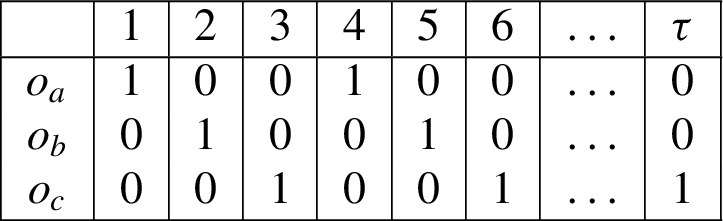
Figure 2 shows an example TP-k assignment $tpa$ for the graph of Example 1 when $k = 2$ and $t_{a} = 2$ . Each table in the figure represents a different k-temporal assignment $ta$ (for the sake of simplicity, we assume those shown are the only possible k-temporal assignments in $TA$ ). Note that $\sum_{ta \in TA} tpa (ta) = 1$ . For any given k-temporal assignment $ta$ , the ith column, with $i \in {1, \dots, τ}$ in the corresponding table represents the k-assignment associated by $ta$ with time point i. Moreover each temporal assignment satisfies Constraints (1) during the analysis period, and for each k-assignment α, $\sum_{v \in V_{obs}} α (v) = k$ .

In addition the defender also generates temporal probabilistic k-assignment to minimize the attacker’s probability of successor the expected damage.
3.3. Temporal probabilistic program induced by the enterprise network

An enterprise network provides important information about the asset values of its vertices, how a vertex can be attacked, and the probability of success. We use APT-programs to combine all this information. We provide a formal transformation from an enterprise network $EN = (V, S, T, V_{obs}, E, asset_val, c_prob)$ to an APT-program $Π_{EN}$ . In addition, this program captures the effects of a k-assignment $ta$ on the enterprise network by using the $unobserved$ atoms present in the activation program $Π_{ta}$ (see Definition 6). Note that these atoms are derived directly from the enterprise network as each vertex is either observed (i.e. has a security software running on it that generates security alerts) or is unobserved (i.e. has no such security software running on it). We use the following example to illustrate the situation.

Example 7.
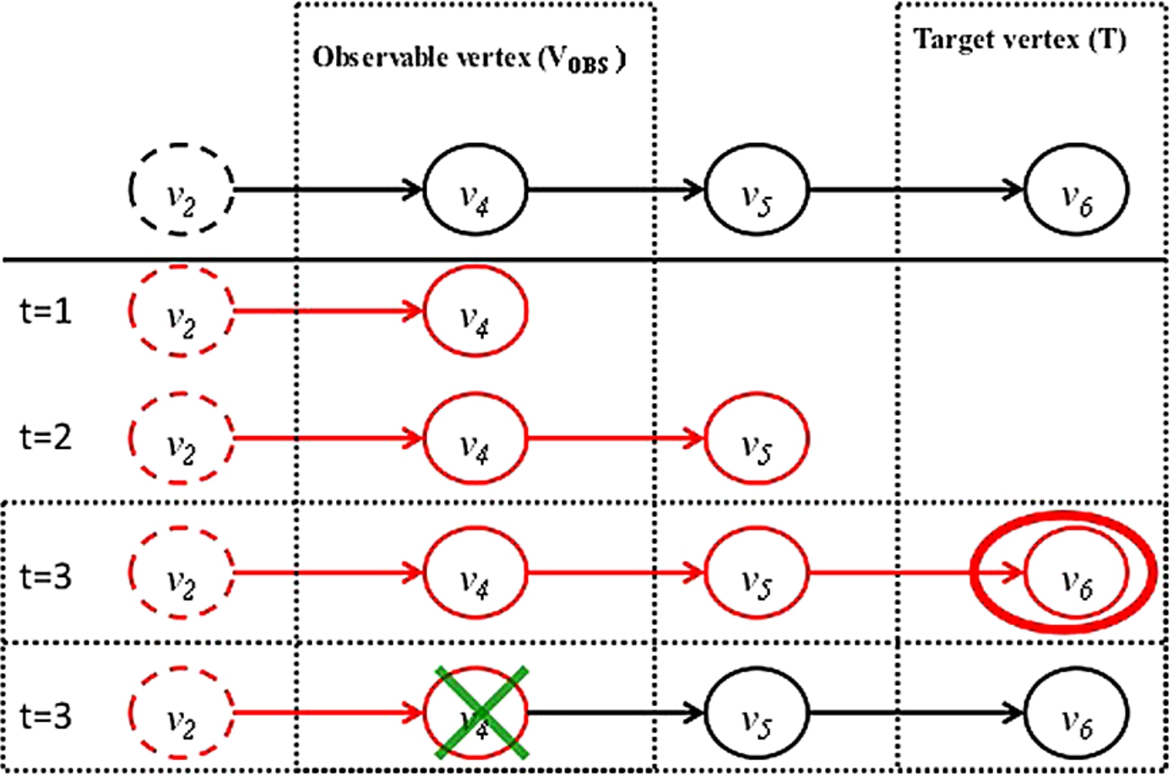
Given sub-network $EN$ in Fig. 1, consider the set $S = {v_{2}, v_{4}, v_{5}, v_{6}}$ of vertices. Suppose $v_{4}$ is the only observable vertex (i.e. the only vertex with a security program running on it that generates security alerts that an analyst working for the MSS service might need to see) and $v_{6}$ is the target. Suppose $v_{2}$ was compromised by the attacker and $T = {0, 1, 2, 3}$ . Figure 3 shows a possible strategy an attacker may use to reach $v_{6}$ . In this strategy, $v_{4}$ is compromised at $t = 1$ , $v_{5}$ at $t = 2$ and $v_{6}$ at $t = 3$ .

If an analyst observed $v_{4}$ at $t = 2$ , he knows that $v_{2}$ must have been previously compromised and that $v_{4}$ can be used to attack other vertices. If he were to somehow disable any vulnerable software in $v_{6}$ (or take other corrective action) at time $t = 2$ , he could potentially stop the attack on $v_{6}$ .

Fig. 3.
Example of an attack.

The preceding example shows that for a vertex v to be compromised at time t, all vertices that could be used to reach it have to be unobserved till time t. We therefore define the program $Π_{EN}$ as follows. This program encodes the enterprise network as an APT-program.
Definition 8 (Encoding an enterprise network as an APT-program ( $Π_{EN}$ )).

$\begin{array}{l} attacked (Ve) : [1.0, X, X^{'}] \leftarrow Ve \in S \land X ⩽ X^{'} \\ \begin{matrix} attacked (Ve) : [⨁_{(v, Ve) \in E} c_prob (v, Ve) * P_{v}, X, X^{'}] \leftarrow & Ve \in V ∖ (V_{obs} \cup S) \land X ⩽ X^{'} \land \\ \underset{(v, Ve) \in E}{⋀} attacked (v) : [P_{v}, X - 1, X^{'}] \end{matrix} \\ \begin{matrix} attacked (Ve) : [⨁_{(v, V_{e}) \in E} c_prob (v, Ve) * P_{v}, X, X^{'}] \leftarrow & Ve \in V_{obs} \land X ⩽ X^{'} \land \\ \underset{(v, V_{e}) \in E}{⋀} attacked (v) : [P_{v}, X - 1, X^{'}] \land \\ ⋀_{t = X}^{X^{'}} unobserved (Ve) : [1.0, t] \end{matrix} \\ attacketTot (Ve) : [⨁_{t \in T} P_{t}] \leftarrow Ve \in T \land \underset{t \in T}{⋀} attacked (Ve) : [P_{t}, t, t] . \end{array}$

A detailed explanation of this APT-program $Π_{EN}$ is in order. We consider the four rules in turn. The first three rules cover the cases when $v \in S$ , $v \in V ∖ (V_{obs} \cup S)$ , and $v \in V_{obs}$ . The last rule estimates the probability that a vertex in $T$ is attacked. The first three rules, whose the heads have the form $attacked (Ve) : [P, X, X^{'}]$ ,8

⁸
Please remember that we allow at most 2 temporal annotations.

define the probability P that a vertex

Ve

is attacked at time X, and that the probability P (for time X) can be used to infer the probability for other vertices at times

X^{'}

greater than X. Thus, these rules whose heads also have two temporal annotations: the first (X) indicates the time X when the event represented by its atom occurs, while the second (

X^{'}

) checks if the probability that an event occurs at a certain time can be used to infer occurrence of another event at another time

X^{'}

The first rule tells us that any vertex that is a source vertex can be attacked with 100% certainty at any time.

The second rule considers a vertex $Ve$ that is neither a source vertex nor a vertex with a security program running on it. Such a vertex can only be compromised after another vertex v that precedes it in the graph was compromised. We assume that this compromise of $Ve$ occurs one time unit before v was compromised.9

⁹

If the defender believes this is not true, he can replace $(X - 1)$ in the body of this rule by some other value $(X - c)$ for some constant $c ⩾ 1$ .

The third rule assigns a proper value to $attacked (Ve)$ considering whether the vertex $Ve$ is observed or not by a security analyst (see Definition 6).

The fourth rule is simple. It says that when a vertex $Ve$ which is a target vertex us attacked, then a new predicate, $AttackedTot (Ve)$ holds with a probability that is a combination of the probabilities that it is attacked at each time point.

It is important to note that without the variable

X^{'}

, is not possible to model the situation described in Example 7 where the defender can stop the attack on the node

v_{6}

by simply monitoring the vertex

v_{4}

at time

t = 2

. If vertex

v_{4}

is monitored at time

t = 2

, then the attack cannot spread to

v_{6}

because at time 3 (

X^{'} = 3

) the node

v_{4}

that was attacked at time

t = 1

(

X = 1

) is not under attack anymore.

Example 8.

Consider the subnetwork in Example 7, and suppose $v_{2}$ is the only source vertex. Then the ground instances of the first rule of $Π_{EN}$ (with possibly true bodies) are the following: $\begin{array}{l} attacked (v_{2}) : [1.0, 0, 0] \leftarrow v_{2} \in S \land 0 ⩽ 0 \\ attacked (v_{2}) : [1.0, 0, 1] \leftarrow v_{2} \in S \land 0 ⩽ 1 \\ attacked (v_{2}) : [1.0, 0, 2] \leftarrow v_{2} \in S \land 0 ⩽ 2 \\ attacked (v_{2}) : [1.0, 0, 3] \leftarrow v_{2} \in S \land 0 ⩽ 3 \\ attacked (v_{2}) : [1.0, 1, 1] \leftarrow v_{2} \in S \land 0 ⩽ 1 \\ attacked (v_{2}) : [1.0, 1, 2] \leftarrow v_{2} \in S \land 1 ⩽ 2 \\ attacked (v_{2}) : [1.0, 1, 3] \leftarrow v_{2} \in S \land 1 ⩽ 3 \\ attacked (v_{2}) : [1.0, 2, 2] \leftarrow v_{2} \in S \land 2 ⩽ 2 \\ attacked (v_{2}) : [1.0, 2, 3] \leftarrow v_{2} \in S \land 2 ⩽ 3 \\ attacked (v_{2}) : [1.0, 3, 3] \leftarrow v_{2} \in S \land 3 ⩽ 3 . \end{array}$

The 2nd rule describes vertices that are neither source vertices nor observable ones. It states that the probability that a vertex $Ve$ is attacked at time X, depends on the probability that at least one vertex in the in-neighborhood of $Ve$ is attacked at time $X - 1$ . This probability is obtained via the t-conorm $⨁_{(v, Ve) \in E} c_prob (v, Ve) * P_{v}$ where $P_{v}$ is the probability that the vertex v is attacked at time $X - 1$ . Moreover, the probability that $V_{e}$ is attacked at time X can be used to infer the probability that other vertices are attacked at time $X^{'}$ .

Example 9.

Continuing with Example 7, we see that $V ∖ (V_{obs} \cup S) = {v_{5}, v_{6}}$ . The appropriate partial ground instances of the second rule of $Π_{EN}$ that could have true bodies are shown below: $\begin{array}{l} attacked (v_{5}) : [p_{45} * P, 1, 1] \leftarrow v_{5} \in V ∖ (V_{obs} \cup S) \land 1 ⩽ 1 \land attacked (v_{4}) : [P, 0, 1] \\ attacked (v_{5}) : [p_{45} * P, 1, 2] \leftarrow v_{5} \in V ∖ (V_{obs} \cup S) \land 1 ⩽ 2 \land attacked (v_{4}) : [P, 0, 2] \\ attacked (v_{5}) : [p_{45} * P, 1, 3] \leftarrow v_{5} \in V ∖ (V_{obs} \cup S) \land 1 ⩽ 3 \land attacked (v_{4}) : [P, 0, 3] \\ attacked (v_{5}) : [p_{45} * P, 2, 2] \leftarrow v_{5} \in V ∖ (V_{obs} \cup S) \land 2 ⩽ 2 \land attacked (v_{4}) : [P, 1, 2] \\ attacked (v_{5}) : [p_{45} * P, 2, 3] \leftarrow v_{5} \in V ∖ (V_{obs} \cup S) \land 2 ⩽ 3 \land attacked (v_{4}) : [P, 1, 3] \\ attacked (v_{5}) : [p_{45} * P, 3, 3] \leftarrow v_{5} \in V ∖ (V_{obs} \cup S) \land 3 ⩽ 3 \land attacked (v_{4}) : [P, 2, 3] \\ attacked (v_{6}) : [p_{56} * P, 1, 1] \leftarrow v_{6} \in V ∖ (V_{obs} \cup S) \land 1 ⩽ 1 \land attacked (v_{5}) : [P, 0, 1] \\ attacked (v_{6}) : [p_{56} * P, 1, 2] \leftarrow v_{6} \in V ∖ (V_{obs} \cup S) \land 1 ⩽ 2 \land attacked (v_{5}) : [P, 0, 2] \\ attacked (v_{6}) : [p_{56} * P, 1, 3] \leftarrow v_{6} \in V ∖ (V_{obs} \cup S) \land 1 ⩽ 3 \land attacked (v_{5}) : [P, 0, 3] \\ attacked (v_{6}) : [p_{56} * P, 2, 2] \leftarrow v_{6} \in V ∖ (V_{obs} \cup S) \land 2 ⩽ 2 \land attacked (v_{5}) : [P, 1, 2] \\ attacked (v_{6}) : [p_{56} * P, 2, 3] \leftarrow v_{6} \in V ∖ (V_{obs} \cup S) \land 2 ⩽ 3 \land attacked (v_{5}) : [P, 1, 3] \\ attacked (v_{6}) : [p_{56} * P, 3, 3] \leftarrow v_{6} \in V ∖ (V_{obs} \cup S) \land 3 ⩽ 3 \land attacked (v_{5}) : [P, 2, 3] \end{array}$ where $p_{45} = c_prob (v_{4}, v_{5})$ and $p_{56} = c_prob (v_{5}, v_{6})$ .

The 3rd rule describes the vertices in $V_{obs}$ . It says that the conditional probability of an observable vertex $Ve$ being attacked at some time $X^{'} ⩾ X$ , given that it is attacked at time X, depends on whether at least one in-neighbor of $Ve$ is attacked (similarly to the 2nd rule). Moreover, it must hold that the vertex $Ve$ is not observed by any analyst during time interval $[X, X^{'}]$ , i.e. $⋀_{t = X}^{X^{'}} unobserved (Ve) : [t]$ .

Example 10.

Example 7 has only one observable vertex $v_{4}$ . The set of ground instances of the 3rd rule that could be true is: $\begin{array}{l} \begin{matrix} attacked (v_{4}) : [p_{24} * P, 1, 1] \leftarrow & v_{4} \in V_{obs} \land 1 ⩽ 1 \land attacked (v_{2}) : [P, 0, 1] \land \\ unobserved (v_{4}) : [1.0, 1] \end{matrix} \\ \begin{matrix} attacked (v_{4}) : [p_{24} * P, 1, 2] \leftarrow & v_{4} \in V_{obs} \land 1 ⩽ 2 \land attacked (v_{2}) : [P, 0, 2] \land \\ unobserved (v_{4}) : [1.0, 1] \land unobserved (v_{4}) : [1.0, 2] \end{matrix} \\ \begin{matrix} attacked (v_{4}) : [p_{24} * P, 1, 3] \leftarrow & v_{4} \in V_{obs} \land 1 ⩽ 3 \land attacked (v_{2}) : [P, 0, 3] \land \\ unobserved (v_{4}) : [1.0, 1] \land unobserved (v_{4}) : [1.0, 2] \land \\ unobserved (v_{4}) : [1.0, 3] \end{matrix} \\ \begin{matrix} attacked (v_{4}) : [p_{24} * P, 2, 2] \leftarrow & v_{4} \in V_{obs} \land 2 ⩽ 2 \land attacked (v_{2}) : [P, 1, 2] \land \\ unobserved (v_{4}) : [1.0, 2] \end{matrix} \\ \begin{matrix} attacked (v_{4}) : [p_{24} * P, 2, 3] \leftarrow & v_{4} \in V_{obs} \land 2 ⩽ 3 \land attacked (v_{2}) : [P, 1, 3] \land \\ unobserved (v_{4}) : [1.0, 2] \land unobserved (v_{4}) : [1.0, 3] \end{matrix} \\ \begin{matrix} attacked (v_{4}) : [p_{24} * P, 3, 3] \leftarrow & v_{4} \in V_{obs} \land 3 ⩽ 3 \land attacked (v_{2}) : [P, 2, 3] \land \\ unobserved (v_{4}) : [1.0, 3] \end{matrix} \end{array}$ where $p_{24} = c_prob (v_{2}, v_{4})$ .

The 4th rule in $Π_{EN}$ defines the probability that a target vertex is attacked during the whole time period $T$ .

Example 11.

Continuing with Example 7, the partial ground rules for the fourth rule in $Π_{EN}$ are: $\begin{matrix} \begin{matrix} attacked (v_{6}) : [\oplus (P_{1}, P_{2}, P_{3})] \leftarrow & v_{6} \in T \land attacked (v_{6}) : [P_{1}, 1, 1] \land attacked (v_{6}) : [P_{2}, 2, 2] \land \\ attacked (v_{6}) : [P_{3}, 3, 3] . \end{matrix} \end{matrix}$

Given a subset $T^{'} \subseteq T$ of target vertices, we wish to compute the probabilities of $Π_{EN} ⊧ ⋀_{v \in T} attacketTot (v)$ , $P_{l} (Π ⊧ ⋀_{v \in T} attacketTot (v))$ and $P_{h} (Π ⊧ ⋀_{v \in T} attacketTot (v))$ . We use Example 7 to illustrate these computations.

Example 12.

Example 7 has two cases: $v_{4}$ is not observed and $v_{4}$ is observed at time 3. In the first case, Definition 6, has the following facts: $\begin{array}{l} unobserved (v_{4}) : [1, 0] \leftarrow \\ unobserved (v_{4}) : [1, 1] \leftarrow \\ unobserved (v_{4}) : [1, 2] \leftarrow \\ unobserved (v_{4}) : [1, 3] \leftarrow . \end{array}$ The “firable” partial ground rules of $Π_{EN}$ are: $\begin{array}{l} \begin{matrix} attacketTot (v_{6}) : [\oplus (P_{1}, P_{2}, P_{3})] \leftarrow & v_{6} \in T \land attacked (v_{6}) : [P_{1}, 1, 1] \land \\ attacked (v_{6}) : [P_{2}, 2, 2] \land attacked (v_{6}) : [P_{3}, 3, 3] \end{matrix} \\ attacked (v_{6}) : [p_{56} * P, 3, 3] \leftarrow v_{6} \in V ∖ (V_{obs} \cup S) \land 3 ⩽ 3 \land attacked (v_{5}) : [P, 2, 3] \\ attacked (v_{5}) : [p_{45} * P, 2, 3] \leftarrow v_{5} \in V ∖ (V_{obs} \cup S) \land 2 ⩽ 3 \land attacked (v_{4}) : [P, 1, 3] \\ \begin{matrix} attacked (v_{4}) : [p_{24} * P, 1, 3] \leftarrow & v_{4} \in V_{obs} \land 1 ⩽ 3 \land attacked (v_{2}) : [P, 0, 3] \land \\ unobserved (v_{4}) : [1.0, 1] \land unobserved (v_{4}) : [1.0, 2] \land \\ unobserved (v_{4}) : [1.0, 3] \end{matrix} \\ attacked (v_{2}) : [1.0, 0, 3] \leftarrow v_{2} \in S \land 0 ⩽ 3 . \end{array}$ If $p_{24} = p_{45} = p_{56} = 1$ then $P_{l} (Π_{EN} \cup Π_{ta} ⊧ attacketTot (v_{4})) = P_{h} (Π_{EN} \cup Π_{ta} ⊧ attacketTot (v_{4})) = 1$ .

However, suppose $v_{4}$ is observed at time 3. Then, the last fact, by Definition 6, becomes $unobserved (v_{4}) : [0.0, 3] \leftarrow$ and the fourth rule assigns 0 to the probability that vertex $v_{4}$ is attacked at time 1 (to use for time 3) and consecutively $P_{l} (Π_{EN} \cup Π_{ta} ⊧ attacketTot (v_{4})) = P_{h} (Π_{EN} \cup Π_{ta} ⊧ attacketTot (v_{4})) = 0$ .

4. Attacker perspective

In the rest of this section, we formally describe how the defender reasons about the attacker. Throughout this paper, when we talk about the attacker’s behavior, what we really mean is how the defender believes the attacker will behave. assuming he, the defender, is playing the role of the attacker. This perspective is quite common in the class of Stackelberg games that are widely used in security. We thus study (the defender’s view of) the attacker’s strategy, study the complexity of the problem of generating good attacks when the defender considers it from the attacker’s point of view, and then present algorithms the defender believes the attacker might use to generate optimal and sub-optimal but good attacks.

4.1. Attacker strategy: Definition and complexity

We first formally define an attacker strategy w.r.t. an arbitrary but fixed enterprise network $EN = (V, S, T, V_{obs}, E, asset_val, c_prob)$ .

Definition 9 (Attack).

Given an enterprise network $EN = (V, S, T, V_{obs}, E, asset_val, c_prob)$ , an attack is a set $atk \subseteq T$ of target vertices.

$atk$ is simply the set of vertices the (defender believes) the attacker wishes to target. We use $ATK$ to denote the set of all possible attacks. We now define the success probability and expected damage associated with an attack.

Definition 10 (Success probability, damage, expected damage of attack).

Given an enterprise network $EN = (V, S, T, V_{obs}, E, asset_val, c_prob)$ .

The lowest and highest success probabilities of an attack $atk$ w.r.t. a k-temporal assignment $ta$ (respectively a k-temporal probabilistic assignment $tpa$ ) are: $\begin{array}{l} \begin{matrix} {psucc}_{l} (atk, ta) & = P_{l} (Π_{EN} \cup Π_{ta} ⊧ \underset{v \in atk}{⋀} attacketTot (v)) \\ = \sum_{ta \in TA} (tpa (ta) \times {psucc}_{l} (atk, ta)) \end{matrix} \\ \begin{matrix} {psucc}_{h} (atk, tpa) & = P_{h} (Π_{EN} \cup Π_{ta} ⊧ \underset{v \in atk}{⋀} attacketTot (v)) \\ = \sum_{ta \in TA} (tpa (ta) \times {psucc}_{h} (atk, ta)) . \end{matrix} \end{array}$

The lowest and highest expected damage caused by attack $atk$ and a k-temporal assignment $ta$ (respectively a k-temporal probabilistic assignment $tpa$ ) are: $\begin{array}{l} \begin{matrix} {exp_dam}_{l} (atk, ta) & = \sum_{v \in atk} P_{l} (Π_{EN} \cup Π_{ta} ⊧ attackedTot (v)) \times asset_val (v) \\ = \sum_{ta \in TA} tpa (ta) \times {exp_dam}_{l} (atk, ta) \end{matrix} \\ \begin{matrix} {exp_dam}_{h} (atk, tpa) & = \sum_{v \in atk} P_{h} (Π_{EN} \cup Π_{ta} ⊧ attackedTot (v)) \times asset_val (v) \\ = \sum_{ta \in TA} tpa (ta) \times {exp_dam}_{h} (atk, ta) . \end{matrix} \end{array}$

Note that if the defender believes that the attacker has a different way of assigning an asset value to a node than the defender, then we can replace $asset_val (v)$ in the two formulas defining expected damage above by ${asset_val}^{'} (v)$ where ${asset_val}^{'}$ is the asset value assigned to vertex v by the attacker.

The following result states that when $ta$ is fixed, the probability of success is anti-monotonic w.r.t. the attack.

Proposition 1.
Suppose $ta$ is a fixed k-temporal assignment Then the lowest and highest success probability of an attacker are anti-monotone w.r.t. the attack, i.e for all ${atk}_{1}$ and ${atk}_{2}$ in $ATK$ such that $\emptyset \subseteq {atk}_{1} \subseteq {atk}_{2}$ :
${psucc}_{l} ({atk}_{1}, ta) ⩾ {psucc}_{l} ({atk}_{2}, ta)$ .

${psucc}_{l} ({atk}_{1}, tpa) ⩾ {psucc}_{l} ({atk}_{2}, tpa)$ .

${psucc}_{h} ({atk}_{1}, ta) ⩾ {psucc}_{h} ({atk}_{2}, ta)$ .

${psucc}_{h} ({atk}_{1}, tpa) ⩾ {psucc}_{h} ({atk}_{2}, tpa)$ .

On the other hand, when we fix a temporal probabilistic assignment $tpa$ , the result below states that the expected damage is monotonic w.r.t. the attack. Proposition 2.
Suppose we fix a k-temporal probabilistic assignment $tpa$ . Then the lowest and highest expected damage of an attacker are monotone w.r.t. the attack, i.e. for all ${atk}_{1}$ and ${atk}_{2}$ in $ATK$ such that ${atk}_{1} \subseteq {atk}_{2}$ we have that
${exp_dam}_{l} ({atk}_{1}, ta) ⩽ {exp_dam}_{l} ({atk}_{2}, ta)$ .

${exp_dam}_{l} ({atk}_{1}, tpa) ⩽ {exp_dam}_{l} ({atk}_{2}, tpa)$ .

${exp_dam}_{h} ({atk}_{1}, ta) ⩽ {exp_dam}_{h} ({atk}_{2}, ta)$ .

${exp_dam}_{h} ({atk}_{1}, tpa) ⩽ {exp_dam}_{h} ({atk}_{2}, tpa)$ .

4.2. Optimal strategies for the attacker

Next, we define three optimization problems that the defender believes the attacker may seek to solve. We study the computational complexity of these problems, and then develop algorithms that the defender believes that attacker may use to solve these problems.

4.3. Optimization problems for the attacker

The three optimization problems for the attacker (as perceived by the defender) are given below. The defender believes the attacker may generate his strategy according to one or the other of these problems.

Definition 11 (Attacker decision problem (At-DP)).

Suppose $EN$ is an enterprise network. The At-DP problem takes as input: (i) a k-temporal probabilistic assignment $tpa$ , (ii) a success probability cutoff χ and (iii) an expected damage cutoff ϵ. It returns “yes” if there exists an attack $atk$ such that ${psucc}_{l} (atk, tpa) ⩾ χ$ and ${exp_dam}_{l} (atk, tpa) ⩾ ϵ$ .

Note that this is an estimate, made by the defender, of the attacker’s success probability if the defender uses a particular temporal probabilistic assignment $ta$ . The same estimate is used in the statement of the following problems.

Definition 12 (Attacker success maximization problem (At-SMP)).

Suppose $EN$ is an enterprise network. The At-SMP problem takes as input: (i) a k-temporal probabilistic assignment $tpa$ , and (ii) an expected damage cutoff ϵ. It returns an attack $atk$ (if one exists) such that ${exp_dam}_{l} (atk, tpa) ⩾ ϵ$ that maximizes ${psucc}_{l} (atk, tpa)$ .

Definition 13 (Attacker damage maximization problem (At-DMP)).

Suppose $EN$ is an enterprise network. The At-DMP problem takes as input: (i) a k-temporal probabilistic assignment $tpa$ , and (ii) a success probability cutoff χ. It returns an attack $atk$ (if one exists) such that ${psucc}_{l} (atk, tpa) ⩾ χ$ that maximizes ${exp_dam}_{l} (atk, tpa)$ .

The decisional variant of the last two problems is called the At-DP problem.

4.4. Complexity results for the attacker

The following result states that the attacker decision problem is intractable.

Theorem 3.
The Attacker decision problem (At-DP) Definition 11 is NP-complete.

Since At-DP problem is NP-complete (Theorem 3), then it is NP-hard, it follows that its optimization versions are NP-hard too. Corollary 1.
Both the optimization problems At-SMP and At-DMP in Definition 12 and Definition 13 are in ${FP}^{NP}$ and NP-hard.

4.5. Using ILP to solve the attacker’s problem

In this section, we present algorithms that leverage integer linear programming (ILP) to solve the attacker problems described above. We note that ILP is a commonly used technique both to solve probabilistic logic programs [42,49,50] and for solving Stackelberg games [7,30,44]. We will use the APT-logic program representation of an enterprise network and the associated APT-logic rules to provide a high-level representation of the adversary’s possible actions, and then automatically generate integer linear programs to capture what is optimal for the attacker. If a security officer for an MSS had to write down this ILP, he would be writing something analogous to assembler code instead of using a high level language – the process would be extremely cumbersome.

In our ILPs, we define some specific variables whose intuitions are summarized in Table 5 (see Appendix C). For each target vertex v in T, we define a binary variable $z_{v} \in {0, 1}$ indicating whether the vertex v belongs to $atk$ ( $z_{v} = 1$ ) or not ( $z_{v} = 0$ ), i.e. indicating whether the attacker chooses to attack vertex v or not. Moreover, for each $ta \in TA$ , we use a real variable ${su}_{ta}$ to represent ${psucc}_{l} (atk, ta)$ and a binary variable ${sub}_{ta}$ to model the min operator in the t-norm (1 if it is the min, 0 otherwise). The ILP named ILP At-DP shown below solves the At-DP problem.10

¹⁰
In order to transform this formulation into one with an objective function, it is enough to use the known ILP trick that relaxes each constraint by adding for a new artificial “slack” variable into each constraint and then setting the objective function to minimize the sum of all the slack variables.

By assuming $tpa$ is modeled by the variables ${z_{v} | v \in T}$ , Constraints (2) and (3) model the fact that ${psucc}_{l} (atk, tpa) ⩾ χ$ and ${exp_dam}_{l} (atk, tpa) ⩾ ϵ$ , respectively. Constraint (2) is based on the variables ${su}_{ta}$ ( $\forall ta \in AS$ ) whose value is equal to $P_{l} (Π_{EN} \cup Π_{ta} ⊧ ⋀_{v \in atk} attackedTot (v)) = min (0, 1 + \sum_{v \in atk} ({psucc}_{l} ({v}, ta) - 1))$ when the Constraints (4), (5), and (6) hold. In particular the variable ${sub}_{ta}$ ( $\forall ta \in AS$ ) is used to model the min operator. If $1 + \sum_{v \in atk} ({psucc}_{l} ({v}, ta) - 1) > 0$ then ${sub}_{ta} = 0$ and ${su}_{ta} = 1 + \sum_{v \in atk} ({psucc}_{l} ({v}, ta) - 1)$ , otherwise ${sub}_{ta} = 1$ and ${su}_{ta} = 0$ . Constraint (3) is straightforward since ${psucc}_{l} ({v}, ta)$ is equal to $P_{l} (Π_{EN} \cup Π_{ta} ⊧ attacketTot (v))$ .

The following result shows how a minor modification to ILP At-DP, together with an appropriate objective function, can help solve both the Attacker Success Maximization Problem (At-SMP) and the Attacker Damage Maximization Problem (At-DMP).

Proposition 4.

Let ILP-SMP (resp. ILP-DMP) be the integer linear program obtained by removing Constraint ( 2 ) (resp. Constraint ( 3 )) from ILP At-DP. Then of maximizing the objective function $\sum_{ta \in AS} tpa (ta) \times {su}_{ta}$ (resp. $\sum_{v \in T} (asset_val (v) * \sum_{ta \in AS} tpa (ta) * {psucc}_{l} ({v}, ta)) \times z_{v}$ ) w.r.t. ILP-SMP (resp. ILP-DMP) solve the optimization problem in Definition 12 (resp. Definition 13 ).

Thus, the defender knows that a savvy attacker can compute the optimal set of attacks to use against a given enterprise by setting up the integer linear programs ILP-SMP and ILP-DMP defined above and then optimizing one of the two objective functions given above. It is up to him whether he wishes to maximize the success probability or whether he wishes to maximize (expected) damage to the enterprise network.

In the real world, it has long been known that players are not rational (i.e. in practice, they do not necessarily do what is optimal for them). Though we do not treat this case theoretically in this paper, our experiments allow us to consider sub-rational actors. Section 6 provides a Monte-Carlo algorithm to simulate attacks that an attacker can launch. The degree of rationality of the attacker is controlled there via two variables – we will discuss this later in Section 6.

5. Optimal strategies for the defender

In the preceding section, the defender places himself in the shoes of the attacker and sees how the attacker may respond to any given temporal assignment. For each such temporal assignment, the attacker has a “best” attack that either maximizes success probability or expected damage. The defender therefore wants to choose the temporal assignment that minimizes the maximal success probability or expected damage as appropriate. This is what we describe below.

We formulate three problems the defender must solve, together with a study of the computational complexity of those problems, and algorithms for the defender to use in order to minimize the attacker’s success probability and/or damage caused (in accordance with the defender’s perception of the attacker).

5.1. Optimization problems for the defender

The first defender optimization problem, Def-DP, returns yes if the defender has a monitoring strategy (temporal probabilistic assignment made by the defender) that keeps both the expected success probability and expected damage below some thresholds.

Definition 14 (Defender decision problem (Def-DP)).

Suppose $EN$ is an enterprise network. The Def-DP problem takes as input: (i) a success probability cutoff χ and (ii) an expected damage cutoff ϵ. It returns “yes” if there exists a k-temporal probabilistic assignment $tpa$ such that for all attacks $atk$ , ${psucc}_{h} (atk, tpa) ⩽ χ$ and ${exp_dam}_{h} (atk, tpa) ⩽ ϵ$ .

The next problem, Def-SMP, tries to find a monitoring strategy that minimizes the success probability of an attacker’s attack, subject to the requirement that the expected damage caused be below a threshold.

Definition 15 (Defender success minimization problem (Def-SMP)).

Suppose $EN$ is an enterprise network. The Def-SMP problem takes as input an expected damage cutoff ϵ. It returns a k-temporal probabilistic assignment $tpa$ (if one exists) such that (i) for all attacks $atk$ ${exp_dam}_{h} (atk, tpa) ⩽ ϵ$ and (ii) $max {{psucc}_{h} (atk, tpa) | atk is an attack}$ is minimized.

The next problem, Def-DMP, tries to find a monitoring strategy for the defender that minimizes the expected damage the attacker causes, subject to the success probability being below a given threshold.

Definition 16 (Defender damage minimization problem (Def-DMP)).

Suppose $EN$ is an enterprise network. The Def-SMP problem takes as input a success probability cutoff ϵ. It returns a k-temporal probabilistic assignment $tpa$ (if one exists) such that (i) for all attacks $atk$ ${psucc}_{h} (atk, tpa) ⩽ ϵ$ and (ii) $max {{exp_dam}_{h} (atk, tpa) | atk is an attack}$ is minimized.

Note that the parameters χ in Definition 15 and ϵ in Definition 16 can be considered optional. For instance, initially, the security manager will find a monitoring strategy minimizing the expected damage (the probability of success) without consider the constraint about the probability of success (the expected damage), i.e. $χ = 1.0$ ( $ϵ = \infty$ ). Once a minimum value of expected damage $e^{*}$ (probability of success $s^{*}$ ) is found, the security manger may want a monitoring strategy that minimizes the probability of success (expected damage) by fixing the expected damage (the probability of success), i.e. $ϵ = e^{*}$ ( $χ = s^{*}$ ).

The result below states that the defender’s decision problem is computationally intractable.

Theorem 5.
The Def-DP problem in Definition 14 is NP-complete.

Since the decisional problem is NP-complete (Theorem 5), it follow that its optimization versions are hard too. Corollary 2.
Both the optimization problems in Definition 15 and Definition 16 are in ${FP}^{NP}$ and NP-hard.

5.2. Using LP to solve the defender’s problem

We now provide a linear program (not an integer LP) LP Def-DP that solves the defender optimization problems Def-DP, Def-SMP, and Def-DMP.11

¹¹
The reader may wonder how an NP-hard problem can be solved via a linear program which is polynomially solvable. The reason there is no inconsistency is because the linear programs we consider such as LP Def-DP are exponential in the size of the original problem Def-DP. Later, we will show how to use column generation methods to significantly improve performance.

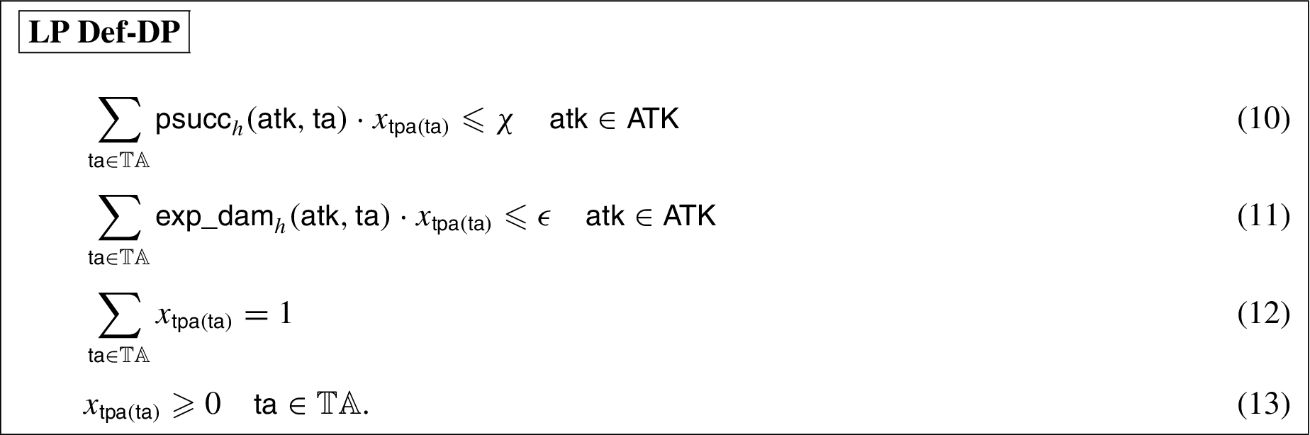
We start by showing a set of linear constraints that models the problem in Definition 14. We associate with each k-temporal assignment $ta \in TA$ , a variable $x_{tpa (ta)}$ representing the (unknown) probability of the temporal assignment $ta$ . We use the set of constraints LP Def-DP. Table 5 provides a succinct explanation of the variables used in the ILPs in this section (see Appendix C).

The first constraint in LP Def-DP says that the expected probability of a successful attack should be below a threshold and likewise, the second constraint says that the expected damage should be less than a threshold. Both these are expected value computations. The third and fourth constraints say that $tpa$ should be a probability distribution.

Proposition 6.

Each solution of the linear program LP Def-DP below is a solution to the defender’s Decision Problem given in Definition 14 (and vice versa).

The main problem with the constraint formulation LP Def-DP is the exponential number of constraints and variables. We have a variable for each $ta \in TA$ , and two constraints of type (10) and (11) for each attack $atk \in ATK$ . The following two propositions show an important result: we can get rid of the exponential number of constraints and replace them with a tractable number of constraints via an alternative encoding. However, the set of variables in the resulting LPs is still intractable. The proposition below states that the set of constraints (10) can be replaced by a tractable number of constraints.

Proposition 7.

The set of Constraints ( 10 ) is equivalent to the following set of constraints: $\begin{matrix} \sum_{ta \in TA} {psucc}_{h} ({v}, ta) \cdot x_{tpa (ta)} ⩽ χ v \in T . \end{matrix}$

A similar result holds for the set of constraints having the form (11).

Proposition 8.

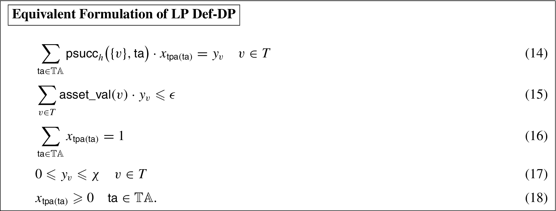
The set of Constraints ( 11 ) is equivalent to the following set of constraints: $\begin{array}{l} \sum_{ta \in TA} {psucc}_{h} ({v}, ta) \cdot x_{tpa (ta)} = y_{v} v \in T \\ \sum_{v \in T} asset_val (v) \cdot y_{v} ⩽ ϵ \\ y_{v} ⩾ 0 v \in T . \end{array}$

By using Proposition 7 and Proposition 8, we obtain the following tractable set of constraints.

An equivalent formulation, that will be useful in Section 5.4, replaces Constraint (14) with the following constraint: $\begin{matrix} (19) & \sum_{ta \in TA} {psucc}_{h} ({v}, ta) \cdot x_{tpa (ta)} ⩽ y_{v} v \in T . \end{matrix}$

Finally, by using Proposition 6, Proposition 7 and Proposition 8, the next results follow in a straightforward manner.

Proposition 9.

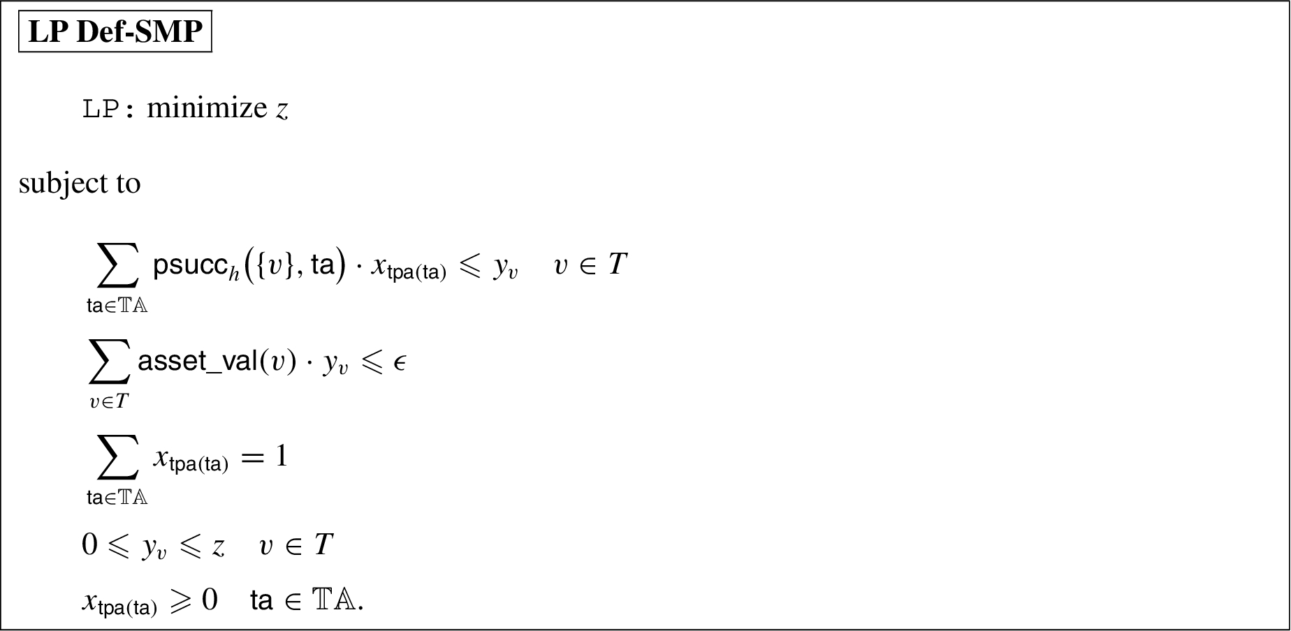
Each solution of the linear program LP Def-SMP below is a solution to the defender’s success minimization problem given in Definition 15 (and vice versa).

Proposition 10.

Each solution of the linear program LP Def-MMP below is a solution to the defender’s damage minimization problem given in Definition 15 (and vice versa).

Though the three LPs given above have a tractable number of constraints, they all have an exponential number of variables. In order to address this problem, we use the column generation technique.

5.3. Column generation problem (CGP)

Column generation is a technique used to solve linear programs that contain a huge number of variables. It works on a restricted formulation of the LP that initially contains some, not all, variables. CGP proceeds iteratively to solve this “restricted problem”. While there exists another variable not present in the restricted LP whose “reduced cost” (defined below) is negative, it adds one such variable to the restricted program and re-solves the resulting LP. This is continued till no such new variable exists. In our case, we insert variables representing the temporal assignments into the reduced program. It is important is to find a new variable with negative reduced cost – this step is calling “solving CGP”.

Definition 17 (Column generation problem (CGP)).

Given the set of dual variables ${d v_{v} | v \in T}$ for the constraints in Line 14, and the dual variable $\hat{d v}$ for the constraint in Line 16, the column generation problem finds a k-temporal assignment $ta$ whose reduced cost ${rc}_{ta}$ is less than 0 where ${rc}_{ta} = - \hat{d v} - \sum_{v \in T} d v_{v} \times {psucc}_{h} ({v}, ta) < 0$ .

Note that $\forall v \in T : d v_{v} ⩽ 0$ because the dual variables associated with the Constraints (19) are less or equal than zero by definition. The following result states that the decisional variant of the CGP, i.e the problem of checking if there exists a temporal assignment $ta$ whose reduced cost is negative, is intractable.

Theorem 11.
The decisional column generation problem is NP-complete.

5.3.1. ILP formulation for CGP

We solve CGP via an integer linear program that models the temporal logic program fixpoint operator $T_{Π}$ defined earlier as well as the k-temporal assignment. This builds upon a long history of work in classical and non-monotonic logic programming where fixpoint operators are captured via linear programs [10].

We consider a restricted version of APT-logic programs whose rules in $groundPG (Π_{EN})$ have the following form: $\begin{matrix} r) a (\dots) : [\oplus_{h} (c_{1}^{r} * X_{1}, \dots, c_{2}^{r} * X_{l}), \dots] \leftarrow \underset{i}{⋀} p x_{i} (\dots) : [X_{i}, \dots] \land \underset{j}{⋀} p c_{j} (\dots) : [1, \dots] \end{matrix}$ where $a (\dots) : [f (X_{1}, \dots, X_{l}), \dots]$ and ${p x_{i} (\dots) : [X_{i}, \dots] | i}$ are atoms where only the probabilistic annotation is not ground, and ${p c_{j} (\dots) : [1, \dots] | j}$ are completely ground atoms. We use $source (Π_{EN})$ to denote the set of all atoms in $groundPG (Π_{EN})$ involving a source vertex in $EN$ (i.e. the atoms in the head of the first rule in $Π_{EN}$ ). For each rule r, we use $bodyPA (r)$ to denote the set of partial ground temporal atoms in the body of r, $bodyG (r)$ denotes the set of the ground atoms in the body. Given an atom a that is a ground atom or an atom where only the probabilistic annotation is not ground, $atomT (a)$ denotes the temporal ground version of a. Furthermore, we assume that for each ground temporal atom a there exists only one ground rule $r_{a}$ s.t. the temporal version of its head is a. It is easy to see that these restrictions perfectly match the last three rules in $Π_{EN}$ , while the first fact rule is mapped by assigning value 1.0 in the interpretation to each ground temporal atom $a \in source (Π_{EN})$ .

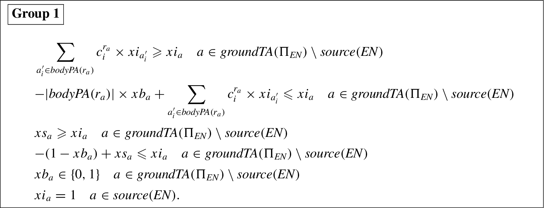
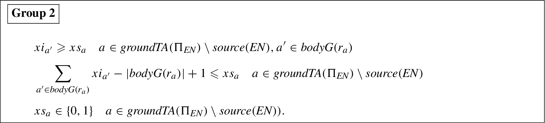
In our ILP formulation, we use a positive real variable $x i_{a}$ for each temporal ground atom a in $groundTA (Π_{EN}) ∖ source (EN)$ representing the value assigned by the interpretation for the atom a. Moreover we use the variable $x s_{a}$ indicating if $⋀_{j} p c_{j} (\dots) : [1, \dots]$ in $r_{a}$ is satisfied by the current interpretation. We then divide the constraints into two groups: Group 1 and Group 2. Group 1 requires that for each atom a, the binary variable $x i_{a}$ is equal to ${\oplus_{h}}_{a_{i}^{'} \in bodyPA (r_{a})} c_{i}^{r_{a}} * x i_{a^{'}}$ if $x s_{a} ≅ 1$ , and 0 otherwise. In this section we do not impose any constraints on variables related to $unobserved ()$ atoms. These variables will represent the output of CGP. The constraints are the following

The variable $x b_{a}$ for each atom $a \in groundTA (Π_{EN})$ is used to model the min operator in the t-conorm and the test on the variable $x s_{a}$ . The constraints in Group 2 require that for each atom $a \in groundTA (Π_{EN}) ∖ source (EN)$ the variable $x s_{a}$ is 1 if for all $a^{'} \in bodyPA (r_{a})$ the value of the current interpretation for $a^{'}$ is equal to 1 (i.e. $x i_{a^{'}} = 1.0$ ) and 0 otherwise.

These two groups of constraints and variables model the fixpoint computation under the assumption that $Π_{EN}$ is acyclic. We will denote all of these constraints as fix-point constraints.

Proposition 12.
Suppose $ta$ is a k-temporal assignment $ta$ . Let $C$ be the set of in constraints Group 1 and Group 2 together with the following constraints $\begin{matrix} x i_{unobserved (v) : [t]} = ta (t) (v) \forall v \in V_{obs}, t \in T . \end{matrix}$ Then: for all $a \in groundTA (Π_{EN}) ∖ source (EN)$ , the value of the variable $x b_{a}$ in all solutions of $C$ is equal to $T_{Π_{EN} \cup Π_{ta}}^{\infty} (a)$ .

5.3.2. Capturing the k-temporal assignment and its reduced cost minimization

In this section, we develop an ILP that uses a binary variable $y b_{v, t}$ for each $v \in V_{obs}$ and $t \in T$ , representing whether the vertex v is monitored at time t ( $y b_{v, t} = 1$ ) or not ( $y b_{v, t} = 0$ ). The formulation is as follows:

where the constraints from Line 21 to Line 24 and variables ${z b_{v, t} | v \in V_{obs}, t \in T}$ are used to model the Constraint (1) in Definition 5.

Proposition 13.
Each solution of the Integer linear program ILP CGP below is a solution to the Column Generation Problem (CGP) Definition 17 (and vice versa).

5.4. Polynomial heuristic algorithm for CGP

We now provide a polynomial heuristic algorithm to solve the CGP. If we obtain a solution with the heuristic algorithm, then we insert the corresponding variable into the restricted program otherwise we call the exact method based on ILP. Let $CH = {(v, t) | v \in V, t \in {1, \dots, | T | - t_{a}}}$ .

Given a set $H \subseteq CH$ , the temporal assignment ${ta}_{H}^{'}$ is such that $\begin{matrix} {ta}_{H}^{'} (t) (v) = \{\begin{matrix} 1 & if \exists t^{'} \in {max (0, t - ta), \dots, t} : (v, t^{'}) \in H \\ 0 & otherwise . \end{matrix} \end{matrix}$

By following the above definitions, Constraint (1) in Definition 5 is automatically satisfied. However, for ${ta}_{H}$ to be a k-temporal assignment, ${ta}_{H}$ has to satisfy the constraint that for each time $t \in T : | {v | v \in V_{obs}, {ta}_{H} (t) (v) = 1} | ⩽ k$ .

We define a function $F : CH \to R$ such that $F (H) = - {rc}_{{ta}_{H}} = \hat{d v} + \sum_{v \in T} d v_{v} \times {psucc}_{h} ({v}, {ta}_{H})$ .

Proposition 14.
The column generation problem can be rewritten as follows: $\begin{matrix} (30) & max {F (H) | \forall t \in T : | {v | \forall v \in V_{obs}, {ta}_{H} (t) (v) = 1} | ⩽ k} . \end{matrix}$
Theorem 15.
The function F is a monotone function, i.e. $(\forall H \subseteq CH) (\forall H^{'} \subset H) : F (H^{'}) ⩽ F (H)$ .

We would have liked F to be submodular so that we could leverage the famous Nemhauser–Wolsey [48] result to generate a polynomial time algorithm with approximation guarantees for CGP. Unfortunately, this is not the case because of the min operator in $\oplus_{h} (x, y) = min (1, x + y)$ .
Example 13.
Consider a simple network with four nodes ${a, b, c, d}$ and the following edges ${(a, b), (a, c), (b, d), (c, d)}$ where $c_prob$ is always 1, the source is a, the target is d, only b and c are observable, $t_{a} = 2$ , $d v = 0$ , $d v_{d} = - 1$ and $T = {1, 2}$ . Consider $H = \emptyset$ , $H^{'} = (b, 1)$ and $h = (c, 1)$ . In this case, $F (H) = F (H^{'}) = F (H \cup {(c, 1)}) = - 1$ and $F (H^{'} \cup {(c, 1)}) = 0$ . Thus F is not submodular because the main condition is violated $F (H \cup {(c, 1)}) - F (H) = 0 ⩽ F (H^{'} \cup {(c, 1)}) - F (H^{'}) = 1$ .

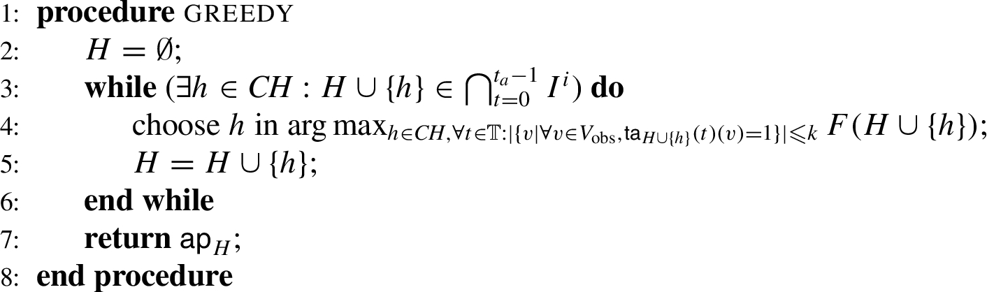
We therefore propose the following heuristic greedy algorithm to solve the CGP problem.

Algorithm 1
GreedyCGP algorithm

Note that since the function F is monotone, the Algorithm 1 increases the value $F (H)$ in each iteration.
6. Monte-Carlo simulation of attacks

In this section, we describe how Monte-Carlo simulation can be used to generate attacks for our experiments.

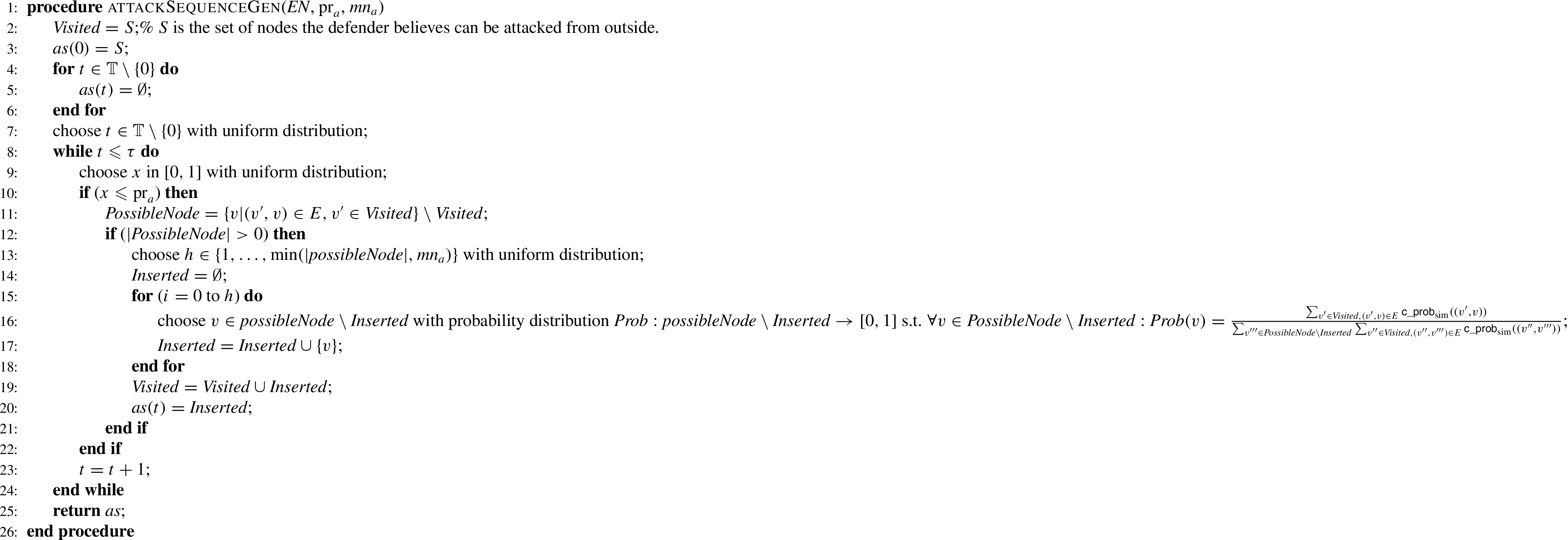
An attack sequence is a function $as : T \to 2^{| V |}$ s.t. for each $t, t^{'} \in T$ , $t \neq t^{'} \to as (t) \cap as (t^{'}) = \emptyset$ . For each time point $t \in T$ , this function assigns a set of nodes attacked at time t. In order to generate this attack sequence we propose a simulation algorithm. Let ${pr}_{a} (t)$ be a probability that the attacker decides to attack new nodes at time t, and let ${mn}_{a}$ the maximum number of nodes that the attacker decides to attack at any given time point. These two parameters control the attacker’s rationality. As ${pr}_{a} (t)$ decreases, for instance, the attacker more prefers to stay in the current situation without additional attacks, which is definitely sub-optimal behavior.

Algorithm 2 generates a random attack sequence. It initializes the set of $Visited$ nodes to the set of source vertices S mentioned in Definition 1 (line 2) and chooses uniformly at random the time t when the attack will start (line 7). Next, the algorithm for each time in ${t, \dots, τ}$ it decides with probability ${pr}_{a}$ to attack some nodes to that time (line 10) and in case, it will compute the possible nodes to attacks (line 11) and how many nodes h will be attacked at that time (line 13). Then in the case the algorithm will attack at that time, for h time it will choose a node to insert in $inserted$ with a specific probability distribution upon $possibleNode ∖ Inserted$ (line 16). After the h iterations it will adds $inserted$ to $visited$ (line 19). At the end, it will return the attack sequence $as$ (line 25).

Algorithm 2

Attack sequence generator

We now define an attack sequence that successfully attacks a target vertex.

Definition 18.

Given an enterprise network $EN$ , an attack sequence $as$ , a temporal assignment $ta$ , a target vertex v, and a time t, v is attacked at time t by $as$ , denoted $(as, ta) ⊧ (v, t)$ , if there exists a sequence $⟨ (v_{1}, t_{1}), \dots, (v_{m}, t_{m}) ⟩$ s.t.

$\forall i \in {1, \dots, m} : v_{i} \in as (t_{i})$ and $v_{m} = v$ and

and $t_{1} ⩽ t_{2} ⩽ \dots ⩽ t_{m}$ and $t_{m} = t$ and

and $\forall i \in {1, \dots, m - 1} : (v_{i}, v_{i + 1}) \in E$ and

and $(\forall i \in {1, \dots, m}) (\forall t^{'} \in {t_{i}, \dots, t_{m}}) : ta (t^{'}) (v_{i}) = 0$ .

(as, ta) ⊧ v

means that vertex v is attacked if

\exists t \in T

such that

(as, ta) ⊧ (v, t)

Since real systems are attacked by several attackers at the same time, we consider a collection $AS$ of attack sequences. We say $(AS, ta) ⊧ v$ if there exists $as \in AS$ s.t. $(as, ta) ⊧ v$ . We define the attack function as follows: $\begin{matrix} attack (AS, ta) = \{\begin{matrix} 1 & \exists v \in T : (AS, ta) ⊧ v \\ 0 & otherwise . \end{matrix} \end{matrix}$ Then, given a set $CAS$ of sets $AS$ of attack sequences, we can estimate the expected probability of success as $\begin{matrix} {psucc}_{sim} (tpa) = \frac{\sum_{AS \in CAS} \sum_{ta \in TA} tpa (ta) \cdot attack (AS, ta)}{| CAS |} \end{matrix}$ and the expected damage as $\begin{matrix} {exp_dam}_{sim} (tpa) = \frac{\sum_{AS \in CAS} \sum_{ta \in TA} tpa (ta) \cdot \sum_{v \in T, (AS, ta) ⊧ v} asset_val (v)}{| CAS |} . \end{matrix}$

7. Mixed, pure, and greedy defender strategies

The preceding section defined approaches based on column generation to solve both the defender’s Success Minimization Problem (Def-SMP) and the defender’s Damage Minimization Problem (Def-DMP) – we call these solutions Mixed-Def-SMP or Mixed-Def-DMP respectively (or just Mixed when the problem being solved is clear from context). In addition, we propose a pure and a greedy strategy for these problems below. These are denoted Pure-Def-SMP, Pure-Def-DMP, and Greedy – the last is common to both problems. Later, we experimentally compared Mixed with both Pure and Greedy for both problems.

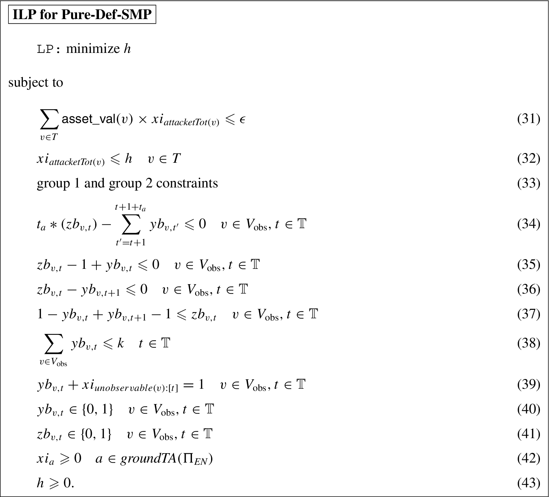
7.1. The PURE strategies

In classical game theory, a pure strategy is one involving no randomization. The Pure-Def-SMP and Pure-Def-DMP returns a pure strategy, i.e. k-temporal assignment. They are defined in the following ways:

Definition 19 (Pure defender success minimization problem (Pure-Def-SMP)).

Suppose $EN$ is an enterprise network. The Pure-Def-SMP problem takes as input an expected damage cutoff ϵ. It returns a k-temporal assignment $ta$ (if one exists) such that (i) for all attacks $atk$ ${exp_dam}_{h} (atk, ta) ⩽ ϵ$ and (ii) $max {{psucc}_{h} (atk, ta) | atk is an attack}$ is minimized.

Definition 20 (Pure defender damage minimization problem (Pure-Def-DMP)).

Suppose $EN$ is an enterprise network. The Pure-Def-SMP problem takes as input a success probability cutoff ϵ. It returns a k-temporal assignment $ta$ (if one exists) such that (i) for all attacks $atk$ ${psucc}_{h} (atk, ta) ⩽ ϵ$ and (ii) $max {{exp_dam}_{h} (atk, ta) | atk is an attack}$ is minimized.

The decisional version for both these problems is as follows.

Definition 21 (Pure defender decision problem (Pure-Def-DP)).

Suppose $EN$ is an enterprise network. The Def-DP problem takes as input: (i) a success probability cutoff χ and (ii) an expected damage cutoff ϵ. It returns “yes” if there exists a k-temporal probabilistic assignment $tpa$ such that for all attack $atk$ , ${psucc}_{h} (atk, tpa) ⩽ χ$ and ${exp_dam}_{h} (atk, tpa) ⩽ ϵ$ .

The result below states that the pure defender decision problem is computationally intractable.

Theorem 16.
The Pure-Def-DP problem in Definition 21 is NP-complete.

Since the decisional problem is NP-complete (Theorem 16), it follow that its optimization versions are hard too.
Corollary 3.
Both the optimization problems in Definition 19 and Definition 20 are in ${FP}^{NP}$ and NP-hard.

Pure-Def-SMP and Pure-Def-DMP can be solved by slight modifications to the ILP formulation used to solve the column generation problem in Section 5.3 – we change the objective function and add some new constraints. The formulation of the ILP for Pure-Def-SMP and Pure-Def-DMP are given below.

Finally the next result follows straightforward Proposition 17.
Each solution of the Integer linear program ILP for Pure-Def-SMP (ILP for Pure-Def-DMP) below is a solution to the defender’s pure success minimization problem given in Definition 19 (pure success minimization problem given in Definition 20 ) and vice versa.

7.2. The greedy strategies

The Greedy method maintains an attacked node list ${Attacked}_{{as}_{i}}$ for each ${as}_{i} \in AS$ as time goes by. (Remember that $AS$ may consist of several simultaneous attacks.) When deciding which observable vertices to protect, Greedy combines all ${Attacked}_{{as}_{i}}$ and selects the vertices with the highest asset values to protect. Of course, this assignment should be done in a manner that is consistent with the minimum $ta$ requirement (cf. Line 13 to Line 19). It is important to notice that in line 22 we remove from the set of nodes previously attacked ${PrevAttacked}_{{as}_{i}}$ the set of nodes $ta (t)$ that are currently monitored.

Algorithm 3

Greedy k-temporal assignment

8. Experiments

This section describes the result of experiments we conducted to assess the efficacy of our algorithms (see Algorithm 3).

8.1. Experimental setting

Code and environment. Our code was implemented in Java with IBM ILOG CPLEX 12.6 for solving (integer) linear programs. All the experiments were run on an Intel Xeon CPU clocked at 2.40 GHz, running Linux, with 24 GB RAM.

Enterprise network data. We tested our algorithms on 15 enterprise networks obtained from three real networks: the first two were networks used in [39], while the third one is the CDX 2009 Network [61] – these networks are denoted EN0, EN1, and EN2 respectively and are described in Table 3. For each real network EN, we generate several virtual enterprise networks ENxD by duplicating the network D times and adding some random edges, where $D \in {1, 2, 4, 6, 8, 10}$ . For instance, EN2x10 denotes the enterprise network EN2 (i.e. the CDX 2009 network) duplicated 10 times, together with some randomly added edges. For each of these networks, we randomly assign asset values for each target node in a range between 10,000 and 200,000 and normalize them to make $\sum_{v \in T} asset_val (v) = 1$ . For each edge e, we set $c_prob (e)$ by randomly selecting a value from $[0.4, 1]$ . We set the value of $t_{a}$ to be in ${2, 3, 5, 10}$ .12

¹²
$t_{a} = 1$ represents the situation where the analyst can immediately identify problems generated with an alert and fix it which is an unlikely situation.

Table 3

Enterprise networks used in experiments. Note that 10 ∼ 25% of V are set to target nodes in EN0x10, EN1x4, EN1x10 and EN2x10

EN	$\| V \|$	$\| E \|$	$\| S \|$	$\| {v \| (v^{'}, v) \in E, v^{'} \in S} \|$	$\| V_{obs} \|$	$\| T \|$
EN0x1	13	50	2	2	11	11
EN0x2	26	110	2	3	24	24
EN0x4	52	230	2	6	50	50
EN0x6	78	350	2	7	76	76
EN0x8	104	470	2	11	102	102
EN0x10	130	588	2	14	128	(13)
EN1x1	8	34	1	4	7	7
EN1x2	16	78	1	5	15	15
EN1x4	32	166	1	8	31	31 or (4)
EN1x6	48	254	1	11	47	47
EN1x8	64	342	1	12	63	63
EN1x10	80	430	1	14	79	(12)
EN2x1	21	102	1	4	20	20
EN2x2	42	224	1	5	41	41
EN2x4	84	468	1	9	83	83
EN2x6	126	712	1	10	125	125
EN2x8	168	956	1	11	167	167
EN2x10	210	1200	1	14	209	(21)

For each enterprise network, we solve the defender’s Success Minimization Problem (Def-SMP) and the defender’s Damage Minimization Problem (Def-DMP) after setting $ϵ, χ \in {0.1, 0.2, \dots, 0.9, 1.0}$ .13

¹³

ϵ and χ are the maximum expected damage and maximum success probability, respectively.

8.2. Experimental results

8.2.1. Quality of protection with Mixed-Def-SMP and Mixed-Def-DMP algorithms as number of analysts and runtime is varied

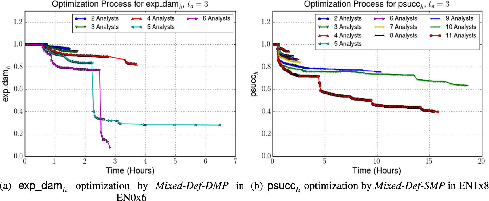
Figure 4 shows the efficacy of the Mixed-Def-SMP and Mixed-Def-DMP in protecting the enterprise network as these algorithms are allowed to run for increasing amounts of time with varying numbers of analysts. In particular, Fig. 4 shows how the expected damage ${exp_dam}_{h}$ and the max attack success probability ${psucc}_{h}$ vary with increased run time of these algorithms. We note that:

After running for about 1.5–2.5 hours (depending on the number of analysts), all algorithm level off in the sense that they do not further reduce expected damage beyond that point.

We note that small changes in the number of available analysts can make a big difference. In particular, when the number of analysts is increased from 4 to 5 or 6, there is a huge drop in the expected damage caused by the attacker. A similar trend holds for probability of success – when going from 10 to 11 analysts, there is a huge drop in the probability of an attack being successful.

8.2.2. Runtime of Mixed-Def-SMP and Mixed-Def-DMP algorithms as enterprise network size and number of analysts is varied

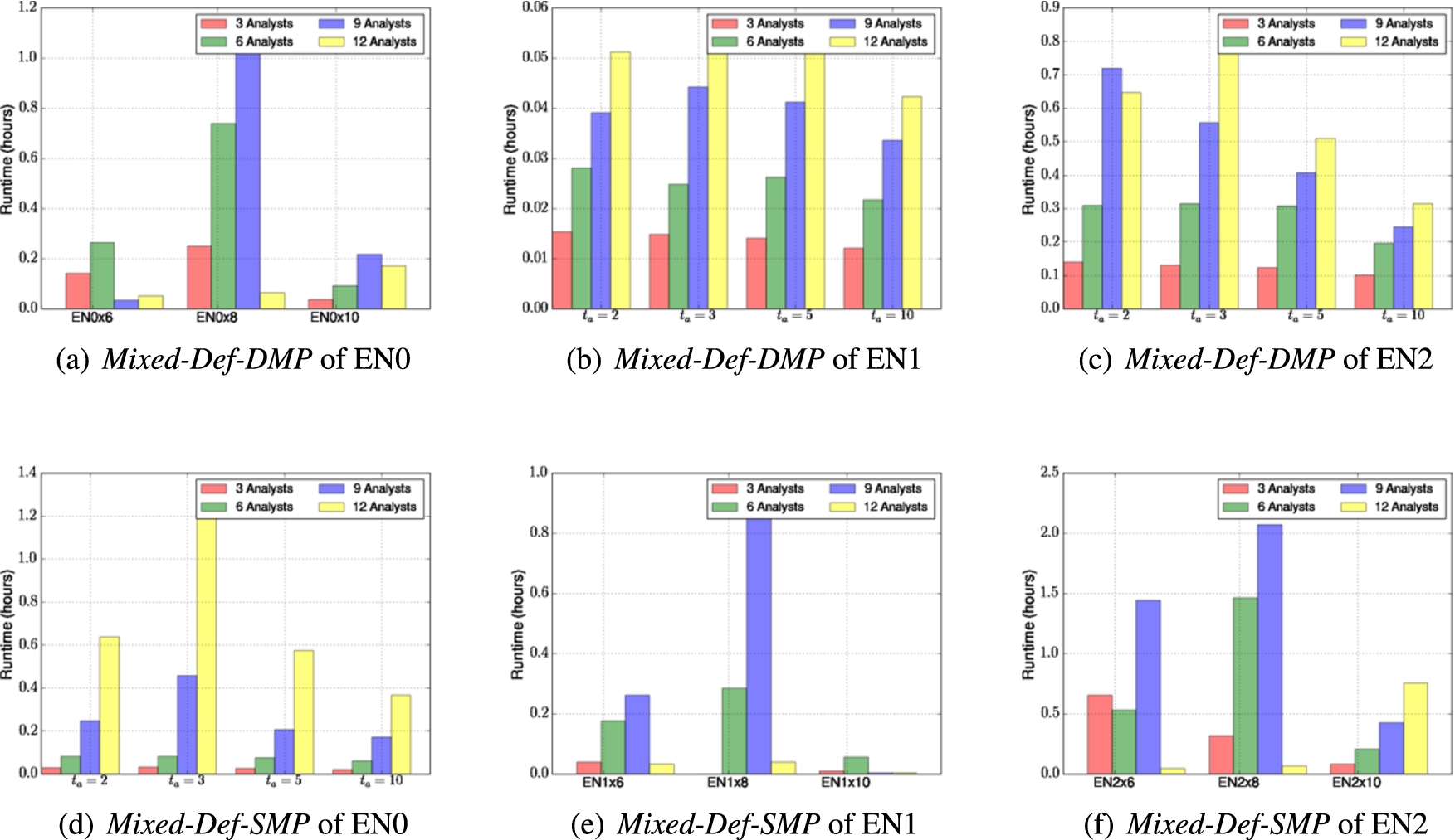
Figure 5 shows the run time of Mixed-Def-DMP and Mixed-Def-SMP. In particular, we see that as we increase the number of analysts, runtime increases, but at a general, mostly linear slope. Similarly, as the size of the enterprise network increases, we see an increased run-time.

Setting $t_{a} = 3$ often led to long runtimes. When $t_{a}$ is either very small (e.g. 2), or very large (e.g. 10), both Mixed-Def-SMP and Mixed-Def-DMP quickly converge to the optimal solution. Mixed-Def-SMP took a longer time than Mixed-Def-DMP in almost all cases because target nodes have different asset values. Using Mixed-Def-DMP, protecting some target nodes can easily lead to a negative reduced cost whereas all target nodes are equally important in Mixed-Def-SMP.

Fig. 4.

Efficacy of defense by Mixed-Def-SMP and Mixed-Def-DMP algorithms as number of analysts and runtime is varied.

Fig. 5.

Runtime of Mixed-Def-SMP and Mixed-Def-DMP algorithms as the size of enterprise networks is varied. (Due to the lack of space, we show for a subset of analyst numbers we had run.)

8.2.3. Column generation step improved by the GreedyCGP algorithm

In order to show the efficacy of the greedy column generation algorithm GreedyCGP, we show how many times on average (by considering all different parameter settings) we avoid calling the expensive exact ILP CGP, because the GreedyCGP is able (by itself) to find a column with negative reduced cost.14

¹⁴
The ILP CGP is called only if GreedyCGP fails to find a column with negative reduced cost.

We then compared the number of columns generated on average by GreedyCGP algorithm and the ILP CGP algorithm. This is summarized in Table 4. We found that the majority of columns are generated by GreedyCGP without using ILP CGP. For example, 88% of columns were found by GreedyCGP and only 12% columns by ILP CGP in EN2x10, and ILP CGP was never called for EN0x1 because we could protect the entire network using only the columns generated by GreedyCGP.

Table 4

The number of columns generated by GreedyCGP and ILP CGP (averaged over all analyst numbers, $t_{a} = 3$ )

EN	Columns generated by GreedyCGP	Columns generated by ILP CGP
EN0x1	7.9	0.0
EN0x2	12.2	1.5
EN0x4	39.8	6.8
EN0x6	104.9	2.8
EN0x8	271.3	7.2
EN0x10	24.4	7.0
EN1x1	8.7	0.5
EN1x2	7.0	2.1
EN1x4	25.1	5.5
EN1x6	72.3	12.4
EN1x8	115.3	13.2
EN1x10	7.6	5.9
EN2x1	11.7	0.4
EN2x2	27.7	1.1
EN2x4	144.6	5.0
EN2x6	280.2	2.2
EN2x8	435.8	2.0
EN2x10	39.2	5.3

8.3. Parameters in defending against multiple attacks

Hereafter, we study the performance of our Mixed, Pure, and Greedy algorithms for the defender’s Damage Minimization Problem and the defender’s Success Minimization Problem in protecting an enterprise network against multiple attacks. For simplicity, we write Mixed and Pure instead of Mixed-Def-SMP, Mixed-Def-DMP. We generate various simulated attacks for each enterprise network by varying the parameters of Algorithm 2 as follows:

$| CAS | = 10000$ . We randomly generated 10,000 collections of sets of attack sequences.

The number of simultaneous attack sequences h ranges from 1 to 20. Each attack sequence $AS$ consists of 1–20 simultaneous attacks.

The probability ${pr}_{a} = 0.75$ . If a vertex u has been attacked at time t, then the attacker attacks a neighbor v of u with 75% probability. (Appendix A reports additional results when ${pr}_{a}$ is selected uniformly at random from the $[0, 1]$ interval.) Due to space reasons, we only report the results of ${pr}_{a} = 0.75$ in the text).

The number of attacks ${mn}_{a}$ is drawn randomly from 2 to 20. In other words, if an attack has already targeted vertex u, attackers target between 2–20 of its neighbors.

${c_prob}_{sim} (u, v) = c_prob (u, v)$ considers the case when attackers behave in the same way as the data used to find k-temporal probabilistic assignment $tpa$ .

${c_prob}_{sim} (u, v) = 1$ means attackers behave differently from the data above, suggesting some random behavior.

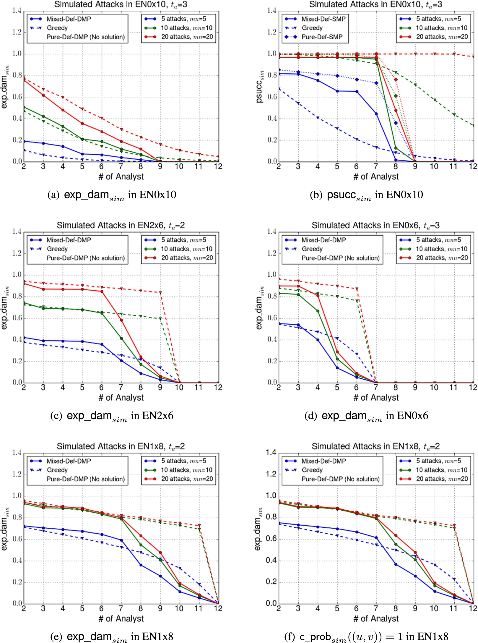
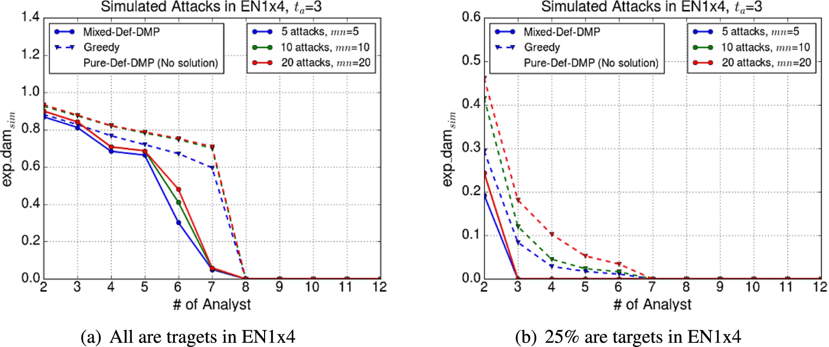
8.4. Defending against multiple attacks: Experimental results

We summarized various charts in Fig. 6 for ${exp_dam}_{sim}$ and ${psucc}_{sim}$ . For all charts of ${exp_dam}_{sim}$ (or ${psucc}_{sim}$ ), we computed the pure and mixed solutions by solving the defender’s Damage Minimization Problem (or the defender’s Success Minimization Problem). For simplicity, we say Mixed and Pure instead of Mixed-Def-SMP, Mixed-Def-DMP, and so on if the experiment result analysis is the case regardless of the problem to solve.

Fig. 6.

Simulated attack results when users behave in accordance with the data: Cases (a)–(e) and differently from the data: Case (f).

Efficacy of Mixed-Def-SMP, Mixed-Def-DMP, and Greedy Algorithms as the Total Number of Simultaneous Attacks and the Number of Analysts are Varied and Attackers Behave Similarly to the Data. Figure 6 shows how the expected damage caused by attacks and the probability of success of attacks vary as the number of analysts and the total number of simultaneous attacks change and when the attackers behave similarly to the data. We specifically make the following observations:

Observation 1. Figure 6(c), (d), (e), and (f) show that the minimum number of analysts to completely protect enterprise networks is the same as the number of neighbors of source vertices15

¹⁵

This is summarized in the column for $| {v | (v^{'}, v) \in E, v^{'} \in S} |$ in Table 3 for each enterprise network.

if all vertices are target vertices and are observable. However, a smaller number of analysts is enough with a clever assignment if the ratio of target vertices to all vertices is reduced. In EN0x10, for example, 9 analysts can protect the entire network from attackers because only 10% of nodes are targets. This phenomenon is explained by the following example.

Example 14.

Consider an enterprise network where the nodes are ${source, o_{a}, o_{b}, o_{c}, v, target}$ and the edges are ${(source, o_{a}), (source, o_{b}), (source, o_{c}), (o_{a}, v), (o_{b}, v), (o_{c}, v), (v, target)}$ . Here $source$ , $target$ are source and target vertices respectively, while $o_{a}$ , $o_{b}$ , $c_{c}$ are observable vertices. Even though $| {v | (v^{'}, v) \in E, v^{'} \in S} | = 3$ in this case, it is possible to obtain a temporal assignment with just one analyst that keeps the enterprise safe. An example of such a temporal assignment is:

When this assignment is used by the defender, the attacker is unable to reach the target before he is detected by an analyst. In this example, this is because there is only one target node which is a certain distance away from the source node. In this case, the attacker needs to attack 2 non-target nodes before he reaches the target.

Observation 2. In all cases, Mixed produces better results than Pure for both ${exp_dam}_{sim}$ and ${psucc}_{sim}$ , which is exactly why we use k-temporal probabilistic assignment $tpa$ rather than temporal assignment $ta$ . With 8 analysts in EN0x10 (Fig. 6(b)), for example, Mixed-Def-SMP is approximately 4 ∼ 5 times better than Pure-Def-SMP. Moreover, in many cases, Pure-Def-DMP was unable to find a solution for the defender’s Damage Minimization Problem because there was no way to achieve the attack success probability less than ϵ only with one k-temporal assignment. In those cases, we omitted the graphs for Pure-Def-DMP.

Observation 3. Mixed and Pure did not show any big improvement on Greedy when analyst numbers were small (e.g. 2 ∼ 4 analysts). This is because in this case, there always exist possible unprotected attack paths. Moreover, Greedy works well if both the number of attacks is small and there are very few analysts. However, when the attack numbers are increased to 10 and $mn = 10$ , Greedy shows poor performance when compared with Mixed.

Efficacy of Mixed-Def-SMP, Mixed-Def-DMP, and Greedy Algorithms as the Total Number of Simultaneous Attacks and the Number of Analysts are Varied and Attackers Behave Differently from the Data. In order to test a slightly different situation, we set ${c_prob}_{sim} ((u, v)) = 1$ , which means attackers behave differently from the data. This may happen in the real world when attackers change their attack strategies from time to time so that previously collected attack statistics become useless. Greedy’s performance is not greatly affected by ${c_prob}_{sim} ((u, v))$ due to its dynamic assignment property. However, though the performance of Mixed was slightly affected, Fig. 6(f) shows no major changes in our conclusions.

Observation 4. As expected, Fig. 7 shows that all three algorithms are greatly affected by the $t_{a}$ values. As $t_{a}$ increases, the performance of all three algorithms decreases. Comparing Fig. 6(e), Fig. 7(c) and Fig. 7(d), we see a big performance degradation from $t_{a} = 2$ to $t_{a} = 3$ . After $t_{a} = 3$ , the performance stabilizes. On the other hand, there exist significant performance changes for ${psucc}_{sim}$ in EN0x10 between $t_{a} = 3$ , Fig. 6(b), and $t_{a} = 5$ , Fig. 7(b). Likewise, $t_{a}$ is one of the key factors to decide performance.

Fig. 7.

Simulated attack results by varying $t_{a}$ values.

Efficacy of Mixed-Def-SMP, Mixed-Def-DMP, and Greedy Algorithms as the Total Number of Target Vertices is Varied. Figure 8 shows the efficacy of our algorithms in defending the enterprise network as the number of target vertices is varied – the figure only reports this for the network EN1x4 – results for other networks are not shown for space reasons, but exhibit similar results. As Fig. 8 shows, 3 analysts were enough to block all attack attempts after randomly setting 15% of vertices as targets, whereas at least 8 analysts were needed if all vertices are targets. All methods showed smaller ${exp_dam}_{sim}$ as target numbers are decreased. Moreover, Mixed was substantially better than Greedy for all analyst numbers in Fig. 8(b).

Fig. 8.

Simulated attack results by varying the number of target vertices.

9. Related work

We divide our related work into 3 parts: (i) work on scheduling of human agents to monitor cybersecurity alerts generated by various cybersecurity programs, (ii) work on the use of logic in computer security in general, and (iii) work on the relationship between logic and optimization which is heavily used in this paper.

9.1. Related work on scheduling human agents to monitor cybersecurity alerts

Intrusion detection has been studied for over three decades [3,26,27]. Most of the early research focused on misuse detection models (developing signatures of known attacks; any matched activity is flagged as a possible attack) or anomaly detection models (characterizing normal behaviors of all users and programs; any significant deviation from the normal profile is considered suspicious). Because the volume of alerts generated by intrusion detection sensors was overwhelming, a great deal of later work focused on developing techniques (based on machine learning [59] or data mining [6], for example) for reducing false positives.

There has been some work that has focused on the requirements of human cybersecurity analysts and ways to improve their efficiency [23,31,64]. The task of a cybersecurity analyst includes examining the alerts generated by an intrusion detection system (IDS) such as SNORT or a Security Information and Event Management (SIEM) tool such as Bro [52] and identifying those that are considered as significant and require further investigation.

In this paper, we view cybersecurity analysts as a resource that must be allocated to the process of examining alerts in an optimal way that minimizes risk while meeting the resource constraint. The constraint on the resource is that an enterprise has an arbitrary, but fixed number security analysts available at any point in time. The goal of this paper is to determine a schedule of alerts to show to each analyst, under the assumption that each analyst takes a fixed amount of time to process an alert. Our notion of risk is that such a schedule must minimize both the expected damage to the system (if, for example, an analyst cannot monitor some alerts) and the probability that an attacker would be successful.

9.2. Related work on use of logic for cybersecurity

The use of logic in cybersecurity was first introduced in the context of security by three authors, all in 1992: [11,14,33]. The first two of these papers looked at the use of deontic logic and deontic logic like constructs to capture what is permitted, what is obligatory, and what is forbidden in terms of access control, while the third looked at the use of logic in order to answer queries to databases without revealing secret information. Much further work looked at database query answering by [13,36,60,62] who studied the problem of answering queries to databases without allowing the user to infer data from the answer that he was not authorized to know.

Later efforts looked at the use of logic for expressing security policies, namely who should be authorized to access a body of data, and who should not, and the conditions under which such access should be granted. Examples of work involving logic for policy expression include [4,35,40,55].

None of these works, however, look at using temporal probabilistic logic in security, nor do they build models of the adversary, nor do they look at the problem of allocating cybersecurity analysts to monitor security alerts generated by security monitoring programs.

9.3. Related work on logic and optimization

Our paper uses a host of integer linear programming methods to solve the problem of effectively allocating security analysts to monitor vertices in an enterprise network. We therefore compare with work at the intersection of logic and optimization. The use of optimization methods for processing logical problems goes back to [41] with a host of successful later work such as [37,54]. Later, Nerode and his co-workers developed methods to use integer programming for computing structures in non-monotonic logic programming [9,10].

A relevant threat was work on constraint logic programming (CLP) [38] which embedded numerical constraints within a logic programming framework. Variants of CLP have been used for cybersecurity research by several authors [22,32,45].

10. Conclusion

Most medium and large enterprises have a small group of personnel who are watching alerts generated by a whole host of diverse programs – intrusion detection programs, firewalls, authentication programs, and others. When the enterprises are large, these programs tend to generate large numbers of alerts with high false positive rates [2].

This paper addresses the problem of assigning cyber-security staff to monitor alerts. As both the attacker and the defender know that the defender cannot successfully monitor all alerts in real-time, we develop a zero-sum game-theoretic framework for this problem. Given an enterprise network, and given a probability distribution of which vertices the defender will protect, we model the attacker as launching a set of attacks (i.e. deciding which vertices in the network to target), so as to either maximize the maximal probability of success of the attack (model 1) or maximize the expected damage caused (model 2). Conversely, the defender tries to find the vertices to protect which will minimize either the maximal probability of a successful attack by the attacker (model 1) or minimize the maximal expected damage by the attacker (model 2). We formalize these as optimization problems and show that they are computationally intractable. For the defender, we develop algorithms that optimize the success probability and expected damage, but because of the previous intractability result, these algorithms are not efficient. In all, we present three algorithms for the defender to use – Pure, Mixed, Greedy. Pure is an exact solution to the problem of which vertices the defender should monitor and when. Mixed is a “mixed” strategy in the common parlance of game theory which means that it uses a probability distribution over pure strategies in order to decide which nodes to protect. As the name suggests, Greedy uses a greedy algorithm.

We ran detailed experiments comparing the efficacy of these three algorithms on one real network, and several synthetic networks derived from the one real network. The Mixed algorithm generally performs the best across the board and delivers good results – both in terms of minimizing the attacker’s success probability and damage caused, and in terms of run time.

Footnotes

Acknowledgments

Parts of this work were funded by the Army Research Office grants W911NF11103, W911NF09102, W911NF-13-1-0421, and W911NF-13-1-0317, by the Office of Naval Research grants N00014-13-1-0703 and N00014-15-1-2007, and by the Maryland Procurement Office contract H98230-14-C-0137.

Experiment with random parameters

In the experiment section, we carefully selected parameters to generate simulated attacks. In some cases, however, characteristics of attacks vary a lot in a collection of attack sequences $AS$ . For that, we create each attack sequence $as \in AS$ after selecting parameters randomly as follows.

Results of same cases shown in the experiment section are reported in Fig. 9. We re-confirm that the proposed methods are the best and Greedy works well only if the number of analysts are small for some enterprise networks such as EN0x10 and EN2x6. In all other cases, the proposed methods always produce the best result regardless of analyst numbers.

Proofs

Variable description table

In the following two tables, we summarize all the variables used for our ILP formulation.

References

K.J.

Ahn and

Guha, Linear programming in the semi-streaming model with application to the maximum matching problem, Information and Computation 222 (2013), 59–79. doi:10.1016/j.ic.2012.10.006.

K.G.

Anagnostakis,

Sidiroglou,

Akritidis,

Xinidis,

Markatos and

A.D.

Keromytis, Detecting targeted attacks using shadow honeypots, in: Proceedings of the 14th Conference on USENIX Security Symposium – Volume 14 (SSYM’05), USENIX Association, Berkeley, CA, USA, 2005, pp. 9–9.

J.P.

Anderson, Computer security threat monitoring and surveillance, Technical report, James P. Anderson Co., Fort Washington, PA, 1980.

C.A.

Ardagna,

Cremonini,

Damiani,

De Capitani di Vimercati and

Samarati, Supporting location-based conditions in access control policies, in: Proceedings of the 2006 ACM Symposium on Information, Computer and Communications Security, ACM, 2006, pp. 212–222.

Azaria,

Richardson,

Kraus and

V.S.

Subrahmanian, Behavioral analysis of insider threat: A survey and bootstrapped prediction in imbalanced data, IEEE Transactions on Computational Social Systems 1(2) (2014), 135–155. doi:10.1109/TCSS.2014.2377811.

Barbara and

Jajodia (eds), Application of Data Mining in Computer Security, Vol. 6, Springer, 2002.

Başar, A tutorial on dynamic and differential games, in: Dynamic Games and Applications in Economics, Springer, 1986, pp. 1–25.

Basin,

Caleiro,

Ramos and

Viganò, Distributed temporal logic for the analysis of security protocol models, Theoretical Computer Science 412(31) (2011), 4007–4043. doi:10.1016/j.tcs.2011.04.006.

Bell,

Nerode,

R.T.

Ng and

V.S.

Subrahmanian, Implementing deductive databases by linear programming, in: Proceedings of the Eleventh ACM SIGACT-SIGMOD-SIGART Symposium on Principles of Database Systems, ACM, 1992, pp. 283–292. doi:10.1145/137097.137892.

10.

Bell,

Nerode,

R.T.

Ng and

V.S.

Subrahmanian, Mixed integer programming methods for computing nonmonotonic deductive databases, Journal of the ACM (JACM) 41(6) (1994), 1178–1215. doi:10.1145/195613.195637.

11.

Bieber and

Cuppens, Expression of confidentiality policies with deontic logic, 1992.

12.

Bishop, What is computer security?, Security & Privacy, IEEE 1(1) (2003), 67–69. doi:10.1109/MSECP.2003.1176998.

13.

Biskup and

P.A.

Bonatti, Lying versus refusal for known potential secrets, Data & Knowledge Engineering 38(2) (2001), 199–222. doi:10.1016/S0169-023X(01)00024-6.

14.

Bonatti,

Kraus and

V.S.

Subrahmanian, Declarative foundations of secure deductive databases, in: Database Theory – ICDT’92, Springer, 1992, pp. 391–406. doi:10.1007/3-540-56039-4_55.

15.

P.A.

Bonatti,

Kraus and

V.S.

Subrahmanian, Foundations of secure deductive databases, IEEE Transactions on Knowledge and Data Engineering 7(3) (1995), 406–422. doi:10.1109/69.390247.

16.

P.A.

Bonatti and

Samarati, Logics for authorizations and security, in: Logics for Emerging Applications of Databases, Springer, 2004, pp. 277–323. doi:10.1007/978-3-642-18690-5_8.

17.

P.P.

Bonissone, Summarizing and propagating uncertain information with triangular norms, International Journal of Approximate Reasoning 1(1) (1987), 71–101. doi:10.1016/0888-613X(87)90005-3.

18.

P.P.

Bonissone, Using T-norm-based uncertainty calculi in a naval situation assessment application, Int. J. Approx. Reasoning 2(3) (1988), 328–329.

19.

Bonneau,

Herley,

P.C.

Van Oorschot and

Stajano, The quest to replace passwords: A framework for comparative evaluation of web authentication schemes, in: Security and Privacy (SP), 2012 IEEE Symposium on, IEEE, 2012, pp. 553–567. doi:10.1109/SP.2012.44.

20.

Boole, An Investigation of the Laws of Thought: On Which Are Founded the Mathematical Theories of Logic and Probabilities, Dover Publications, 1854.

21.

Common Weakness Scoring System, 2011, https://cwe.mitre.org/.

22.

Corin and

Etalle, An Improved Constraint-Based System for the Verification of Security Protocols, Springer, 2002.

23.

D’Amico and

Whitley, The real work of computer network defense analysts: The analysis roles and processes that transform network data into security situation awareness, in: Proceedings of the Workshop on Visualization for Computer Security, 2008, pp. 19–37.

24.

Datta,

Derek,

J.C.

Mitchell and

Pavlovic, A derivation system and compositional logic for security protocols, Journal of Computer Security 13(3) (2005), 423–482. doi:10.3233/JCS-2005-13304.

25.

Dekhtyar,

M.I.

Dekhtyar and

V.S.

Subrahmanian, Temporal probabilistic logic programs, in: ICLP,

De Schreye, ed., MIT Press, 1999, pp. 109–123.

26.

D.E.

Denning, An intrusion-detection model, in: Proceedings of IEEE Symposium on Security and Privacy, Oakland, CA, 1986, pp. 118–131.

27.

D.E.

Denning, An intrusion-detection model, IEEE Trans. Software Eng. 13(2) (1987), 222–232. doi:10.1109/TSE.1987.232894.

28.

Desrosiers and

M.E.

Lübbecke, A Primer in Column Generation, Springer, 2005.

29.

DeTreville, Binder, a logic-based security language, in: Proceedings. 2002 IEEE Symposium on Security and Privacy, IEEE, 2002, pp. 105–113. doi:10.1109/SECPRI.2002.1004365.

30.

J.P.

Dickerson,

G.I.

Simari,

V.S.

Subrahmanian and

Kraus, A graph-theoretic approach to protect static and moving targets from adversaries, in: Proceedings of the 9th International Conference on Autonomous Agents and Multiagent Systems: Volume 1-Volume 1, International Foundation for Autonomous Agents and Multiagent Systems, 2010, pp. 299–306.

31.

R.F.

Erbacher and

S.E.

Hutchinson, Extending case-based reasoning to network alert reporting, in: 2012 ASE International Conference on Cyber Security, 2012, pp. 187–194. doi:10.1109/CyberSecurity.2012.31.

32.

Eronen and

Zitting, An expert system for analyzing firewall rules, in: Proceedings of the 6th Nordic Workshop on Secure IT Systems (NordSec 2001), 2001, pp. 100–107.

33.

Glasgow,

MacEwen and

Panangaden, A logic for reasoning about security, ACM Transactions on Computer Systems (TOCS) 10(3) (1992), 226–264. doi:10.1145/146937.146940.

34.

R.L.

Graham,

E.L.

Lawler,

J.K.

Lenstra and

A.H.G.

Rinnooy Kan, Optimization and approximation in deterministic sequencing and scheduling: A survey, Annals of Discrete Mathematics 5 (1979), 287–326. doi:10.1016/S0167-5060(08)70356-X.

35.

J.Y.

Halpern and

Weissman, Using first-order logic to reason about policies, ACM Transactions on Information and System Security (TISSEC) 11(4) (2008), 21.

36.

M.J.

Hasan, Belief reasoning in MLS deductive databases, ACM SIGMOD Record 28(2) (1999), 109–120.

37.

Hooker, Logic-Based Methods for Optimization: Combining Optimization and Constraint Satisfaction, Vol. 2, John Wiley & Sons, 2011.

38.

Jaffar and

J.-L.

Lassez, Constraint logic programming, in: Proceedings of the 14th ACM SIGACT-SIGPLAN Symposium on Principles of Programming Languages (POPL ’87), ACM, New York, NY, USA, 1987, pp. 111–119. doi:10.1145/41625.41635.

39.

Jajodia,

Noel,

Kalapa,

Albanese and

Williams, Cauldron: Mission-centric cyber situational awareness with defense in depth, in: Proceedings of the Military Communications Conference (MILCOM 2011), 2011.

40.

Jajodia,

Samarati,

M.L.

Sapino and

V.S.

Subrahmanian, Flexible support for multiple access control policies, ACM Transactions on Database Systems (TODS) 26(2) (2001), 214–260. doi:10.1145/383891.383894.

41.

R.G.

Jeroslow, Computation-oriented reductions of predicate to propositional logic, Decision Support Systems 4(2) (1988), 183–197. doi:10.1016/0167-9236(88)90128-5.

42.

Kern-Isberner and

Lukasiewicz, Combining probabilistic logic programming with the power of maximum entropy, Artificial Intelligence 157(1) (2004), 139–202. doi:10.1016/j.artint.2004.04.003.

43.

Kim and

M.H.

Kang, Determining asset criticality for cyber defense, Naval Research Laboratory (2011).

44.

Korzhyk,

Yin,

Kiekintveld,

Conitzer and

Tambe, Stackelberg vs. Nash in security games: An extended investigation of interchangeability, equivalence, and uniqueness, J. Artif. Intell. Res. (JAIR) 41 (2011), 297–327.

45.

Li and

J.C.

Mitchell, Datalog with constraints: A foundation for trust management languages, in: Practical Aspects of Declarative Languages, Springer, 2003, pp. 58–73. doi:10.1007/3-540-36388-2_6.

46.

J.W.

Lloyd, Foundations of Logic Programming, 2nd edn, Springer, 1987.

47.

Mell,

Scarfone and

Romanosky, Common vulnerability scoring system, Security Privacy, IEEE 4(6) (2006), 85–89.

48.

G.L.

Nemhauser,

L.A.

Wolsey and

M.L.

Fisher, An analysis of approximations for maximizing submodular set functions – I, Mathematical Programming 14(1) (1978), 265–294. doi:10.1007/BF01588971.

49.

Ng and

V.S.

Subrahmanian, Probabilistic logic programming, Information and Computation 101(2) (1992), 150–201. doi:10.1016/0890-5401(92)90061-J.

50.

N.J.

Nilsson, Probabilistic logic, Artificial Intelligence 28(1) (1986), 71–87. doi:10.1016/0004-3702(86)90031-7.

51.

Paruchuri, Playing games for security: An efficient exact algorithm for solving Bayesian Stackelberg games, in: AAMAS, 2008.

52.

Paxson, Bro: A system for detecting network intruders in real-time, Computer Networks 31(23–24) (1999), 2435–2463. doi:10.1016/S1389-1286(99)00112-7.

53.

Rahmani,

Sahli and

Kamoun, DDoS flooding attack detection scheme based on F-divergence, Computer Communications 35(11) (2012), 1380–1391. doi:10.1016/j.comcom.2012.04.002.

54.

Raman and

I.E.

Grossmann, Modelling and computational techniques for logic based integer programming, Computers & Chemical Engineering 18(7) (1994), 563–578. doi:10.1016/0098-1354(93)E0010-7.

55.

Samarati and

De Capitani di Vimercati, Access control: Policies, models, and mechanisms, in: Foundations of Security Analysis and Design, Springer, 2001, pp. 137–196. doi:10.1007/3-540-45608-2_3.

56.

Serra,

Jajodia,

Pugliese,

Rullo and

V.S.

Subrahmanian, Pareto-optimal adversarial defense of enterprise systems, ACM Transactions on Information and System Security (TISSEC) 17(3) (2015), 11.

57.

Shakarian,

Parker,

G.I.

Simari and

V.S.

Subrahmanian, Annotated probabilistic temporal logic, ACM Trans. Comput. Log. 12(2) (2011), 14.

58.

Shakarian,

G.I.

Simari and

V.S.

Subrahmanian, Annotated probabilistic temporal logic: Approximate fixpoint implementation, ACM Trans. Comput. Log. 13(2) (2012), 13.

59.

Sommer and

Paxson, Outside the closed world: On using machine learning for network intrusion detection, in: Proceedings of IEEE Symposium on Security and Privacy, 2010, pp. 305–316.

60.

Stouppa and

Studer, Data privacy for ALC knowledge bases, in: Logical Foundations of Computer Science, Springer, 2009, pp. 409–421. doi:10.1007/978-3-540-92687-0_28.

61.

USMA, 2009, http://www.usma.edu/crc/SitePages/DataSets.aspx.

62.

Winslett,

Smith and

Qian, Formal query languages for secure relational databases, ACM Transactions on Database Systems (TODS) 19(4) (1994), 626–662. doi:10.1145/195664.195675.

63.

Yu,

Zhou,

Jia,

Guo,

Xiang and

Tang, Discriminating DDoS attacks from flash crowds using flow correlation coefficient, IEEE Transactions on Parallel and Distributed Systems 23(6) (2012), 1073–1080.

64.

Zimmerman, The Strategies of a World-Class Cybersecurity Operations Center, The MITRE Corporation, 2014.

Using temporal probabilistic logic for optimal monitoring of security events with limited resources

Abstract

Keywords

1. Introduction

2.1. Enterprise networks

Definition 1 (Enterprise network).

2 A defender might simply set S to the most weakly protected vertices in the enterprise, while he might set T to contain all vertices that contain information valuable to the defender.

2.2.1. Syntax of APT-logic programs

5 We will also assume that APT-rule bodies can contain built-in conditions c (e.g. 2 > 1 or v ∈ T ). I ⊧ c if c is true under the pre-interpreted meaning of these constraints as in constraint logic programming [38].

3.1. Defender strategy: k-temporal assignments

3.2. k-temporal probabilistic assignment

Definition 7 (TP-k assignment).

8 Please remember that we allow at most 2 temporal annotations.

4.1. Attacker strategy: Definition and complexity

Definition 9 (Attack).

Definition 10 (Success probability, damage, expected damage of attack).

4.3. Optimization problems for the attacker

Definition 11 (Attacker decision problem (At-DP)).

Definition 12 (Attacker success maximization problem (At-SMP)).

Definition 13 (Attacker damage maximization problem (At-DMP)).

4.4. Complexity results for the attacker

5.1. Optimization problems for the defender

Definition 14 (Defender decision problem (Def-DP)).

Definition 15 (Defender success minimization problem (Def-SMP)).

Definition 16 (Defender damage minimization problem (Def-DMP)).

Definition 17 (Column generation problem (CGP)).

Theorem 11. The decisional column generation problem is NP-complete. 5.3.1. ILP formulation for CGP

Proposition 13. Each solution of the Integer linear program ILP CGP below is a solution to the Column Generation Problem (CGP) Definition 17 (and vice versa). 5.4. Polynomial heuristic algorithm for CGP

7.1. The PURE strategies

Definition 19 (Pure defender success minimization problem (Pure-Def-SMP)).

Definition 20 (Pure defender damage minimization problem (Pure-Def-DMP)).

Definition 21 (Pure defender decision problem (Pure-Def-DP)).

8.1. Experimental setting

12 t a = 1 represents the situation where the analyst can immediately identify problems generated with an alert and fix it which is an unlikely situation.

8.2.1. Quality of protection with Mixed-Def-SMP and Mixed-Def-DMP algorithms as number of analysts and runtime is varied

8.2.2. Runtime of Mixed-Def-SMP and Mixed-Def-DMP algorithms as enterprise network size and number of analysts is varied

14 The ILP CGP is called only if GreedyCGP fails to find a column with negative reduced cost.

8.4. Defending against multiple attacks: Experimental results

9.1. Related work on scheduling human agents to monitor cybersecurity alerts

9.2. Related work on use of logic for cybersecurity

9.3. Related work on logic and optimization

10. Conclusion

Footnotes

Acknowledgments

Experiment with random parameters

Proofs

Variable description table

References

²
A defender might simply set S to the most weakly protected vertices in the enterprise, while he might set T to contain all vertices that contain information valuable to the defender.

⁵
We will also assume that APT-rule bodies can contain built-in conditions c (e.g. $2 > 1$ or $v \in T$ ). $I ⊧ c$ if c is true under the pre-interpreted meaning of these constraints as in constraint logic programming [38].

⁸
Please remember that we allow at most 2 temporal annotations.

Theorem 11.
The decisional column generation problem is NP-complete.

5.3.1. ILP formulation for CGP

Proposition 13.
Each solution of the Integer linear program ILP CGP below is a solution to the Column Generation Problem (CGP) Definition 17 (and vice versa).

5.4. Polynomial heuristic algorithm for CGP

¹²
$t_{a} = 1$ represents the situation where the analyst can immediately identify problems generated with an alert and fix it which is an unlikely situation.

¹⁴
The ILP CGP is called only if GreedyCGP fails to find a column with negative reduced cost.