Efficient protocols for oblivious linear function evaluation from ring-LWE 1

Abstract

An oblivious linear function evaluation protocol, or OLE, is a two-party protocol for the function $f (x) = a x + b$ , where a sender inputs the field elements a, b, and a receiver inputs x and learns $f (x)$ . OLE can be used to build secret-shared multiplication, and is an essential component of many secure computation applications including general-purpose multi-party computation, private set intersection and more.

In this work, we present several efficient OLE protocols from the ring learning with errors (RLWE) assumption. Technically, we build two new passively secure protocols, which build upon recent advances in homomorphic secret sharing from (R)LWE (Boyle et al. in: EUROCRYPT 2019, Part II (2019) 3–33 Springer), with optimizations tailored to the setting of OLE. We upgrade these to active security using efficient amortized zero-knowledge techniques for lattice relations (Baum et al. in: CRYPTO 2018, Part II (2018) 669–699 Springer), and design new variants of zero-knowledge arguments that are necessary for some of our constructions.

Our protocols offer several advantages over existing constructions. Firstly, they have the lowest communication complexity amongst previous, practical protocols from RLWE and other assumptions; secondly, they are conceptually very simple, and have just one round of interaction for the case of OLE where b is randomly chosen. We demonstrate this with an implementation of one of our passively secure protocols, which can perform more than 1 million OLEs per second over the ring $Z_{m}$ , for a 120-bit modulus m, on standard hardware.

Keywords

Oblivious linear evaluation two-party computation cryptographic protocols ring learning with errors zero-knowledge arguments

1. Introduction

Oblivious linear function evaluation, or OLE, is a two-party protocol between a sender, with input $a, b \in F$ , and a receiver, who inputs $x \in F$ and receives $y = a x + b$ . OLE is an arithmetic generalization of oblivious transfer to a larger field $F$ , since OLE over $F_{2}$ can be seen as equivalent to oblivious transfer on the messages $z_{0}$ , $z_{1}$ by setting $a = z_{0} + z_{1}$ and $b = z_{0}$ , so the receiver learns $y = z_{x}$ . Similarly to oblivious transfer, OLE can be used in constructions of secure two-party and multi-party computation, and is particularly useful for the setting of securely computing arithmetic circuits over $F$ [4,30,32,37], where OT tends to be less efficient. As well as general secure computation protocols, OLE can be used to carry out specific tasks like private set intersection [34], secure matrix multiplication and oblivious polynomial evaluation [45,48].

OLE can be constructed from a range of “public-key” type assumptions. In the simplest, folklore construction, the receiver encrypts its input x using a linearly homomorphic encryption scheme and gives this to the sender. Using the homomorphic properties of the scheme, the sender computes an encryption of $y = a x + b$ and sends this back to the receiver to decrypt. This approach can be instantiated with Paillier encryption or lattice-based encryption based on the learning with errors (LWE) [47] or RLWE assumptions [42], and has been implicitly used in several secure multi-party computation protocols [14,39,44]. There are also constructions of OLE from coding-theoretic assumptions [33,37,45] which mostly rely on the hardness of decoding Reed–Solomon codes in certain parameter regimes with a high enough noise rate. These constructions are asymptotically efficient, but so far have not been implemented in practice, to the best of our knowledge. For the special (and easier) case of vector-OLE, which is a large batch of many OLEs with the same input x from the receiver, there are efficient constructions from more standard coding-theoretic assumptions over general codes, which also have good performance in practice [4,16,17,48].

Despite the fact there are many existing constructions of OLE, either implicit or explicit in the literature, very few of these works study the practical efficiency of OLE in its own right (except for the special case of vector-OLE). Instead, most of the aforementioned works either focus on the efficiency of higher-level primitives such as secure multi-party computation, or mainly discuss asymptotic efficiency rather than performance in practice. In this work, we advocate for the practical study of OLE as a standalone primitive. This has the benefits that it can be plugged into any higher-level application that needs it in a modular way, potentially simplifying analysis and security proofs compared with a more monolithic approach.

1.1. Our contributions

We present and study new OLE protocols with security based on the ring learning with errors (RLWE) assumption, with passive and active security. Our passively secure protocols are very simple, consisting of just one message per party, and our most efficient variant achieves the lowest communication complexity of any practical (implemented) OLE protocol we are aware of, requiring around half the bandwidth of previous solutions. We add active security using zero-knowledge proofs, which have a low amortized complexity when performing a large number of OLEs, giving only a small communication overhead over the passive protocols. To adapt existing zero-knowledge proof techniques to our protocols, we have to make several modifications, and describe a new amortized proof of knowledge that can be used to show a batch of secret-key (R)LWE ciphertexts is well-formed (previous techniques only apply to public-key ciphertexts).

We have implemented and benchmarked our most efficient passively secure protocol, and show it can compute more than 1 million OLEs per second on a standard laptop, over a $\approx 120$ -bit ring $Z_{m}$ where m is the product of two CPU word-sized primes. The communication cost per OLE is around 4 elements of $Z_{m}$ per party, and the amortized complexity of our actively secure protocol is almost the same, when computing a large enough number of OLEs. This is almost half the communication cost of previous protocols based on RLWE, and less than 25% of the cost of an actively secure protocol based on oblivious transfer and noisy Reed–Solomon encodings [33].

It is also worth noting that this work corresponds to the extended version of [9]. In particular, the list of new added material includes: (1) detailed proofs for the main results obtained in Sections 3 and 4, (2) a formal description of the missing functionalities in [9], (3) a full description of the considered computational problems and commitment schemes (Section 2), (4) additional details on the existing protocols used for comparison (Section 1.4), and (5) additional details on the zero-knowledge arguments used to make the proposed protocols actively secure (Section 5).

1.2. Outline

In Section 1.3 below, we present an overview of the main techniques in our constructions. We then describe some preliminaries in Section 2. Section 3 contains our OLE protocols based on public-key RLWE encryption, which only require a standard public key infrastructure as a setup assumption. In Section 4, we present more efficient protocols which reduce communication using secret-key encryption, and a more specialized setup assumption. Then, in Section 5, we present details on the zero-knowledge arguments which are used to make the previous protocols actively secure. Finally, in Section 6, we analyze the concrete efficiency of our solutions, compare this with previous OLE protocols, and present implementation results for our most efficient passively secure protocol.

1.3. Techniques

Our protocols construct a symmetric variant of OLE, where one party, Alice, inputs a field element $u \in F$ , the other party, Bob, inputs $v \in F$ , and the parties receive random values α and β (respectively) such that $α + β = u \cdot v$ . This can easily be used to construct an OLE by having the sender, say Alice, one-time-pad encrypt her additional input using α, allowing Bob to correct his output accordingly. In this formulation, OLE is also equivalent to producing an additive secret-sharing of the product of two private inputs; this type of secret-shared multiplication is an important building block in multi-party computation protocols, for instance in constructing Beaver multiplication triples [12]. In our protocols, we first create OLEs over a large polynomial ring $R_{m} = Z_{m} [X] / (X^{N} + 1)$ , which comes from the RLWE assumption, and then convert each OLE over $R_{m}$ to a batch of N OLEs over $Z_{m}$ , for some prime modulus m, using packing techniques from homomorphic encryption [49].

Our point of departure is the recent homomorphic secret sharing scheme by Boyle et al. [20], based on LWE or RLWE. Homomorphic secret sharing is a form of secret sharing in which shares can be computed upon non-interactively, such that the parties end up with an additive secret sharing of the result of the computation. HSS was first constructed under the DDH assumption [19] and variants of threshold and multi-key fully homomorphic encryption [29], followed by the more efficient lattice-based construction of [20], which supports homomorphic computation of branching programs (or, “restricted multiplication” circuits where every multiplication gate must involve at least one input wire). Note that any “public-key” type two-party HSS scheme that supports multiplication leads to a simple OLE protocol: each party sends a secret-sharing of its input, then both parties multiply the shares to obtain an additive share of the product.

1.3.1. Efficient OLE from a public-key setup

Our first construction can be seen as taking the HSS scheme of Boyle et al. and optimizing it for the specific functionality of OLE. When plugging in their scheme to perform OLE, a single share from one party consists of two RLWE ciphertexts: one encrypting the message, and one encrypting a function of the secret key, which is needed to perform the multiplication. Our first observation is that, in the setting of OLE where we have two parties who each have one of the inputs to be multiplied, we can reduce this to just one ciphertext per party, where Alice sends an encryption of her input u multiplied by a secret key, and Bob sends an encryption of his input. Both of these ciphertexts, including the one dependent on the secret key, can be created from a standard public-key infrastructure-like setup where Alice and Bob have each others’ RLWE public keys, thanks to a weak KDM security property of the scheme. This gives a communication complexity of two $R_{q}$ elements per party, for a RLWE ciphertext modulus q, to create a single ring-OLE over $R_{m}$ . We can also obtain a further saving by sending one party’s ciphertext at a smaller modulus $p < q$ .

1.3.2. Reducing communication with a dedicated setup

Our second protocol considers a different setup assumption, where the parties are assumed to have access to a single OLE over $R_{q}$ , which gives them secret shares of the product of two RLWE secret keys. With this, we are able to replace the public-key RLWE ciphertexts from the previous protocol with secret-key ciphertexts, which can be of size just one ring element instead of two. This cuts the overall communication in half, and also reduces computational costs.

1.3.3. Achieving active security

To obtain security against active corruptions, we need to ensure that both parties’ RLWE ciphertexts are correctly generated, in particular, that the small “error” polynomials used as encryption randomness were generated correctly (and not too large). For a public key RLWE encryption, this boils down to proving knowledge of a short vector $s \in Z_{q}^{n}$ , such that $A s = c$ where $A$ , $c$ are public values defined by the RLWE public key and ciphertext, respectively. In practice, we do not know efficient methods of proving the above statement. Instead, we can obtain good amortized efficiency when proving knowledge for many such relations of the form $\begin{matrix} (1) & A {\overline{s}}_{i} = c_{i} \end{matrix}$ for the same matrix $A$ , where now the secret ${\overline{s}}_{i}$ may have slightly larger coefficients than the original secret $s_{i}$ . This overhead is known as the soundness slack parameter, and comes from the fact that a dishonest prover can sometimes make the proof succeed even when $s_{i}$ is slightly larger than the claimed bound. Efficient amortized proofs for (1) have been given in several works [7,24,26,40], most recently with a communication overhead that is independent of the number of relations being proven [5].

Proving correctness of a batch of public-key RLWE ciphertexts can be essentially done by proving a batch of relations of the form in (1), allowing use of these efficient amortized proofs. To achieve active security in our public-key OLE protocol, we use a slightly modified version of the proof from [5], by allowing different size bounds to be proven for different components of $s_{i}$ . This gives us tighter parameters for the encryption scheme.

On the other hand, for our second protocol, things are not so straightforward. To see why, recall that a batch of secret-key RLWE ciphertexts have the form: $\begin{matrix} (2) & (a_{i}, a_{i} \cdot s + e_{i} + (q / p) \cdot x_{i}) \end{matrix}$ Here, $a_{i}$ is a random element in the polynomial ring $R_{q} = Z_{q} [X] / (X^{N} + 1)$ , $e_{i}$ is a small error value in $R_{q}$ , and $s \in R_{q}$ is the secret key. We want to prove that both s and $e_{i}$ have small coefficients.

The problem is, since $a_{i}$ is different for each ciphertext, these cannot be expressed in the form of (1), since they are not linear in a fixed public value. This was not the case for the public-key setting, where every ciphertext is linear in the fixed public key; here, by switching to a secret-key encryption scheme to improve efficiency, we can unfortunately no longer apply the amortization techniques of [5].

Furthermore, there is a second obstacle, since we now have a special preprocessing phase which gives out shares of $s_{A} \cdot s_{B}$ , for the parties’ RLWE secret keys $s_{A}$ and $s_{B}$ . These must be the same secret keys that are used to produce the encryptions, and to ensure this, we also have to tie these together into the ZK proof statement.

To work around these issues, we perform two steps. Firstly, we modify the preprocessing so that each party gets a commitment to its secret key, under a suitable homomorphic commitment scheme (which can also be based on lattices [8]). We then design a new proof of knowledge, which proves knowledge of short $(s, e_{i}, x_{i})$ satisfying (2) with similar amortized efficiency to the proof from [5] for (1). Our proof simultaneously guarantees the secret s is the same s that was committed to in the preprocessing, leveraging the homomorphic properties of the commitment scheme.

1.4. Previous works

1.4.1. OLE from additively homomorphic encryption (AHE)

There is a standard approach to building OLE using linearly homomorphic encryption, where $P_{Alice}$ sends $Enc (u)$ to $P_{Bob}$ , who multiplies this with his input v and adds it to $Enc (β)$ for a random $β \in R_{m}$ . For example, this is the method that is implicitly used in the BDOZ [14] and LowGear [39] protocols for actively secure multi-party computation. One drawback of this method, seen in [14], is that to obtain active security, $P_{Bob}$ needs to prove that he multiplied v correctly into the ciphertext sent by $P_{Alice}$ . This proof of correct multiplication is prohibitively more expensive than proofs of plaintext knowledge, since we do not know of any efficient way to amortize a large batch of them. The LowGear protocol [39] avoids the proof of correct multiplication (while still using a proof of plaintext knowledge from $P_{Alice}$ ) by assuming an additional property of the RLWE encryption scheme called “enhanced CPA” security. This is implied by linear-only encryption, a non-falsifiable assumption used in some zero-knowledge constructions [15].

We evaluate this approach in the “AHE” row of Table 1 below, using parameters based on [39].

1.4.2. OLE from RLWE

Concurrently and independently to our work, an efficient instantiation of the AHE-based template described above is presented in [28], essentially using the LPR encryption scheme as described here. To achieve circuit privacy, the authors in [28] do not rely on traditional “noise drowning” techniques. Instead, the authors devise a more efficient method involving “quotient-and-rounding”. This method reduces the sizes of the ciphertexts and allows for cheaper arithmetic.

1.4.3. OLE from somewhat homomorphic encryption (SHE)

Another approach is to use a somewhat (or partially) homomorphic encryption scheme that supports one multiplication, as well as addition, such as BGV [21]. This method has been used to create multiplication triples in many protocols in the SPDZ family [25,26]. To use this to create OLE, each party first sends an encryption of its input u or v, and then multiply the ciphertexts homomorphically. Next, one party sends an encryption of a random value, which is added to this before being decrypted towards the other party with a distributed decryption protocol. This requires 3 ciphertexts to be sent in all, plus one additional $R_{q}$ element for the distributed decryption, where one party sends its “partial decryption” to the other party, who decrypts the result.2

²
This has slightly lower costs than the SPDZ protocol, since we have simplified the distributed decryption for the two-party OLE setting.

We evaluate this approach in row “SHE” of Table 1, using SHE parameters from the Overdrive variant of SPDZ [39].

1.4.4. OLE from noisy Reed–Solomon encodings (RS)

Another approach is based on oblivious transfer and noisy encodings via Reed–Solomon codes [33,37,45]. Here, the protocol of Ghosh et al. [33] has the best concrete efficiency, and achieves active security almost for free on top of previous passive protocols using simple consistency check. The protocol has not been implemented, but according to estimates from [30], an optimistic choice of parameters for the underlying security assumption leads to a communication cost of 32 field elements per OLE. This still leads to a higher communication cost than our protocols. Note that although the other protocols, being based on RLWE encryption, will likely have similar computational costs, we cannot easily compare the computational efficiency of the RS protocol, since it has not been implemented.

1.4.5. Other OLE protocols

There are several other ways of constructing OLE which are not presented in Table 1, which we now briefly discuss here. Recently, Rathee et al. implemented passively secure protocols for Beaver triple generation over rings using RLWE [46]. These are based on the AHE approach described above, except they also use a CRT optimization where the plaintext space is reduced by using several ciphertexts with different plaintext moduli. This optimization is better suited to their setting with multiplication over general rings mod $2^{k}$ , and does not seem to give a benefit for our setting of a large prime plaintext space.

As mentioned earlier, we can also use Paillier encryption to build OLE from linearly homomorphic encryption, and add active security using either zero-knowledge proofs [14] or a common reference string [23]. However, Paillier ciphertexts are very large (at least 4096 bits) and have a high computational overhead, since exponentiations are in many settings much more costly than polynomial operations in RLWE. It may be advantageous to use Paillier when only a few OLEs are desired, but in the amortized setting it seems unlikely to be competitive. OLE can also be constructed from string oblivious transfer, with Gilboa’s method [35]. Using OT extension [36] this can be quite cheap computationally [38], but has a much higher communication cost that is quadratic in the field bit length, instead of linear for all the protocols in Table 1, and around an order of magnitude higher than our protocol.

Finally, Boyle et al. [18] combined homomorphic secret sharing with a PRG based on the hardness of solving multivariate quadratic equations, to produce a large batch of n Beaver triples or OLEs with $o (n)$ communication. This interesting approach clearly has much lower communication than our methods, but it only achieves such low communication when producing a very large number of triples (more than $2^{30}$ ), so will not be suitable for many applications. Furthermore, its computational efficiency is much worse than our protocol.

2. Preliminaries

In this section we introduce some preliminaries and notation we will use. As basic notation, we write $α ⋆ β$ to denote the component-wise product of the vectors $α$ , $β$ .

2.1. Rings & rounding

Let q be an odd integer and $N = 2^{r}$ be a power of two. We define the ring $R : = Z [X] / ⟨ X^{N} + 1 ⟩$ as well as $R_{q} = R / ⟨ q ⟩$ as the reduction of the polynomials of $R$ modulo q. Representing the coefficients of $f \in R_{q}$ uniquely by its representatives from $[- (q - 1) / 2, (q - 1) / 2]$ we define $‖ f ‖_{\infty}$ as the largest norm of any coefficient of f when considered over the above interval. We define by $U (R)$ the uniform distribution over the finite set R and furthermore let $S_{β} = {x \in R ∣ ‖ x ‖_{\infty} ⩽ β}$ .

We now introduce the computational problems we use over $R_{q}$ , which are Ring-LWE, Module-LWE and Module-SIS. We use Ring-LWE in our basic OLE protocols, while Module-LWE and -SIS are used for our zero-knowledge argument with homomorphic commitments.

Definition 1 (Ring-LWE).

Let $R_{q}$ be a ring as defined above, $n \in N^{+}$ and $σ \in R^{+}$ . Let $D_{σ}$ be a discrete Gaussian distribution over $R_{q}$ with standard deviation σ, and $D_{sk}$ be some secret key distribution over $R_{q}$ . We say that an algorithm $A$ has advantage ϵ in solving the ${RLWE}_{n, σ, D_{sk}}$ problem if $\begin{array}{l} | Pr [b = 1 ∣ a \leftarrow U (R_{q}^{n}), e \leftarrow D_{σ}^{n}, s \leftarrow D_{sk}, b \leftarrow A (a, a \cdot s + e)] \\ - Pr [b = 1 ∣ a \leftarrow U (R_{q}^{n}), u \leftarrow U (R_{q}^{n}), b \leftarrow A (a, u)] | ⩾ ϵ \end{array}$

Definition 2 (Module-LWE).

Let $R_{q}$ be a ring as defined above, $n, k \in N^{+}$ . The ${MLWE}_{n, k, β}$ problem asks to distinguish the distribution $[\begin{matrix} I_{n} & A^{'} \end{matrix}] \cdot y$ for a short $y$ , from the uniform distribution when given $A^{'}$ . We say that an algorithm $A$ has advantage ϵ in solving the ${MLWE}_{n, k, β}$ problem if $\begin{array}{l} | Pr [b = 1 ∣ A^{'} \leftarrow U (R_{q}^{n \times (k - n)}) \land y \leftarrow U (S_{β}^{k}) \land b \leftarrow A (A^{'}, [\begin{matrix} I_{n} & A^{'} \end{matrix}] \cdot y)] \\ - Pr [b = 1 ∣ A^{'} \leftarrow U (R_{q}^{n \times (k - n)}) \land u \leftarrow U (R_{q}^{n}) \land b \leftarrow A (A^{'}, u)] | ⩾ ϵ \end{array}$

The Module-LWE problem is widely believed to be hard for polynomial-time distinguishers when $y$ is sampled from a discrete Gaussian distribution over $R$ with large enough standard deviation. The version of Module-LWE we give here has a more aggressive error distribution, but is often used in practice.

A related well-known problem is called Module-SIS.

Definition 3 (Module-SIS).

Let $R_{q}$ be a ring as defined above and $n, k \in N^{+}$ . The ${MSIS}_{n, k, β}$ problem asks to find a short vector $y$ with $‖ y ‖_{\infty} ⩽ β$ satisfying $[\begin{matrix} I_{n} & A^{'} \end{matrix}] \cdot y = 0^{n}$ when given a random $A^{'}$ . We say that an algorithm $A$ has advantage ϵ in solving the ${MSIS}_{n, k, β}$ problem if $\begin{matrix} Pr [y \in S_{β}^{k} \land [\begin{matrix} I_{n} & A^{'} \end{matrix}] \cdot y = 0^{n} ∣ A^{'} \leftarrow U (R_{q}^{n \times (k - n)}) \land 0 \neq y \leftarrow A (A^{'})] ⩾ ϵ . \end{matrix}$

2.1.1. Rounding

We define by ${⌊ f ⌉}_{p}$ the scaling of each coefficient of f by $p / q$ over the reals and then rounding to the nearest integer in $[- (p - 1) / 2, (p - 1) / 2]$ respectively. A simple but useful result we will use throughout our protocols is the following.

Lemma 1.
Let $p | q$ , $x \leftarrow R_{q}^{n}$ and $y = x + e mod q$ for some $e \in R_{q}^{n}$ with $‖ e ‖_{\infty} < B < q / p$ . Then ${{Pr [⌊ y ⌉}_{p} \neq ⌊ x ⌉}_{p} mod p] ⩽ \frac{2 n p N B}{q}$ .
Proof.
It suffices to consider the case $n = 1$ and $R_{q} = Z_{q}$ , since, by the union bound, the general case can be obtained by multiplying the probability obtained in this particular case by $N \cdot n$ .

Let $x \in Z_{q}$ be uniformly random, let $e \in Z_{q}$ be bounded in norm by B, and let $y = x + e mod q$ . Let E be the event ${{⌊ y ⌉}_{p} \neq ⌊ x ⌉}_{p} mod p$ . To bound the probability of E notice that, due to the fact that $| e | < B$ , e cannot change the nearest integer to x unless at least one of these coefficients lies in a ball of radius $(p / q) B$ centered at $k + \frac{1}{2}$ for some integer k. This condition is equivalent to x lying in a ball of radius B centered at $\frac{q}{p} \cdot (k + \frac{1}{2})$ for some integer k. Since $x \in Z_{q}$ is uniformly random, the probability of this event is upper bounded by $2 B / (q / p) = 2 B p / q$ . □

2.2. Gaussian distributions and simulatability

Definition 4.
The continuous normal distribution over $R^{m}$ centered at $v \in R^{m}$ with standard deviation $σ \in R$ is defined by the function $\begin{matrix} ρ_{v, σ}^{m} (x) = {(\frac{1}{\sqrt{2 π σ^{2}}})}^{m} exp (\frac{- ‖ x - v ‖_{2}^{2}}{2 σ^{2}}) . \end{matrix}$

If $v = 0$ then we just write $ρ_{σ}^{m} (x)$ . For a countable set $S \subset R^{m}$ we furthermore define $ρ_{σ}^{m} (S) = \sum_{x \in S} ρ_{σ}^{m} (x)$ .
Definition 5.
The discrete normal distribution over $Z^{m}$ centered at $v \in Z^{m}$ with standard deviation $σ \in R^{m}$ is defined as $\begin{matrix} D_{v, σ}^{m} (x) = ρ_{v, σ}^{m} (x) / ρ_{σ}^{m} (Z^{m}) . \end{matrix}$

Throughout this work we apply $D$ to vectors from $R^{k}$ in which case we mean that $D_{σ} {(x)}^{k} = D_{σ}^{N k} (\overline{x})$ with $\overline{x} \in Z^{N k}$ being the coefficient-wise embedding of $R^{k}$ into $Z^{N k}$ . We similarly consider sampling $R$ -elements from $D_{σ}$ as sampling each coefficient independently from this distribution.

In order to use random variables sampled according to the aforementioned distribution we have to be able to estimate the size of its values. The following statement allows doing so:
Lemma 2 (See Lemma 4.4 of [40]).

For any $k > 1$ , $\begin{matrix} Pr [‖ x ‖_{2} > k σ \sqrt{m} ∣ x \leftarrow D_{σ}^{m}] < k^{m} exp (\frac{m}{2} (1 - k^{2})) . \end{matrix}$

Rejection sampling for product distributions. We will have to perform rejection sampling on vectors whose elements are distributed according to different Gaussian distributions (in particular, they can have different standard deviations). Throughout this work we will use the following

Lemma 3 (Generalizes Theorem 4.6 of [40]).

Let $k \in N^{+}$ and for $i \in [k]$ let $V_{i} \subseteq Z^{m_{i}}$ such that all elements of $V_{i}$ have norm less than $T_{i}$ , $σ_{i} \in R$ such that $σ_{i} = α T_{i}$ and $h_{i} : V_{i} \to R$ be a probability distribution. If $α > 0$ and $M = exp (12 / α + 1 / (2 α^{2}))$ then the following algorithm $A$ :

$v_{1} \leftarrow h_{1}$ , …, $v_{k} \leftarrow h_{k}$

$x_{1} \leftarrow D_{v_{1}, σ_{1}}^{m_{1}}$ , …, $x_{k} \leftarrow D_{v_{k}, σ_{k}}^{m_{k}}$

Output $(x_{1}, \dots, x_{k}, v_{1}, \dots, v_{k})$ with probability $min (\prod_{i \in [k]} \frac{D_{σ_{i}}^{m_{i}} (x_{i})}{M D_{v_{i}, σ_{i}}^{m_{i}} (x_{i})}, 1)$

is within statistical distance

2^{- 100 + log k} / M

of the distribution of the following algorithm

F

$v_{1} \leftarrow h_{1}$ , …, $v_{k} \leftarrow h_{k}$

$x_{1} \leftarrow D_{σ_{1}}^{m_{1}}$ , …, $x_{k} \leftarrow D_{σ_{k}}^{m_{k}}$

Output $(x_{1}, \dots, x_{k}, v_{1}, \dots, v_{k})$ with probability $1 / M^{k}$

where

A

outputs something with probability at least

{(\frac{1 - 2^{- 100}}{M})}^{k}

In order to prove Lemma 3, we make use of the following Theorem, which was proved by Lyubashevsky [40] and lies at the core of many lattice-based constructions:

Theorem 1 (See Theorem 4.6 of [40]).

Let $V \subseteq Z^{m}$ such that all elements of V have norm less than T, $σ \in R$ such that $σ = ω (T \sqrt{log m})$ and $h : V \to R$ be a probability distribution. Then there exists a constant $M = O (1)$ such that the distributions of the following algorithm $A$ :

$v \leftarrow h$

$x \leftarrow D_{v, σ}^{m}$

Output $(x, v)$ with probability $min (\frac{D_{σ}^{m} (x)}{M D_{v, σ}^{m} (x)}, 1)$

is within statistical distance

2^{- ω (log m)} / M

of the distribution of the following algorithm

F

$v \leftarrow h$

$x \leftarrow D_{σ}^{m}$

Output $(x, v)$ with probability $1 / M$

where

A

outputs something with probability at least

\frac{1 - 2^{- ω (log m)}}{M}

For concreteness, if $σ = α T$ for $α > 0$ then $M = exp (12 / α + 1 / (2 α^{2}))$ , meaning that the output of $A$ is within statistical distance $2^{- 100} / M$ of $F$ and that $A$ outputs something with probability at least $\frac{1 - 2^{- 100}}{M}$ .

We can now use the aforementioned theorem to prove Lemma 3:

Proof.
We perform the experiment from Theorem 1 for each of the k components using discrete Gaussian distributions $D_{σ_{i}}^{m_{i}}$ in the process. Since α is fixed among all components, then in particular the constant M will be the same across all k individual experiments. By a union bound, we obtain the statistical distance $2^{- 100 + log k} / M$ by adding up all k identical terms. The fact that $F$ outputs the vector with probability at least ${((1 - 2^{- 100}) / M)}^{k}$ follows by the independence of the k experiments. □

2.3. Ring-LWE based encryption scheme

In this work we use basic ideas from RLWE-based encryption, particularly in our public-key based construction from Section 3. We describe here a simplified version of the public-key encryption scheme from [42], which we refer to as $LPR$ . The key generation, encryption and decryption procedures are defined as follows:

Gen (a)

On input a public random $a \in R_{q}$ , first sample $s \leftarrow D_{sk}$ and $e \leftarrow D_{σ}$ . Output $sk = (s)$ and $pk = (a, b)$ where $b = a \cdot s + e$ .

{Enc}_{p, q} (pk, x)

On input $pk \in R_{q}^{2}$ and $x \in R_{p}$ , sample $w \leftarrow D_{sk}$ , $e_{0}, e_{1} \leftarrow D_{σ}$ and output $(c_{0}, c_{1})$ , where $c_{1} = - a \cdot w + e_{1}$ and $c_{0} = b \cdot w + e_{0} + (q / p) \cdot x$ .

Dec (sk, (c_{0}, c_{1}))

Compute $x^{'} = c_{0} + s \cdot c_{1} mod q$ , and output ${x = ⌊ x^{'} ⌉}_{p} mod p$ .3

³
Our protocols do not directly use the decryption algorithm, but our simulator in the proof of Theorem 3 does.

Notice that this works if the total noise

e = s \cdot e_{1} + e \cdot w + e_{0}

is bounded by

p / 2 q

On top of these standard procedures, we also use an algorithm $KDMEnc$ which produces an encryption of $x \cdot s$ , where s is the secret key. As observed in [20] (and implicit in [3,22]), this can be done using only the public key by adding the message to the second component of an encryption of zero. ${KDMEnc}_{p, q} (pk, x)$ :

Sample $w \leftarrow D_{sk}$ , $e_{0}, e_{1} \leftarrow D$ and output $(c_{0}, c_{1})$ , where $c_{1} = (q / p) \cdot x - a \cdot w + e_{1}$ and $c_{0} = b \cdot w + e_{0}$ .

2.4. Oblivious linear function evaluation

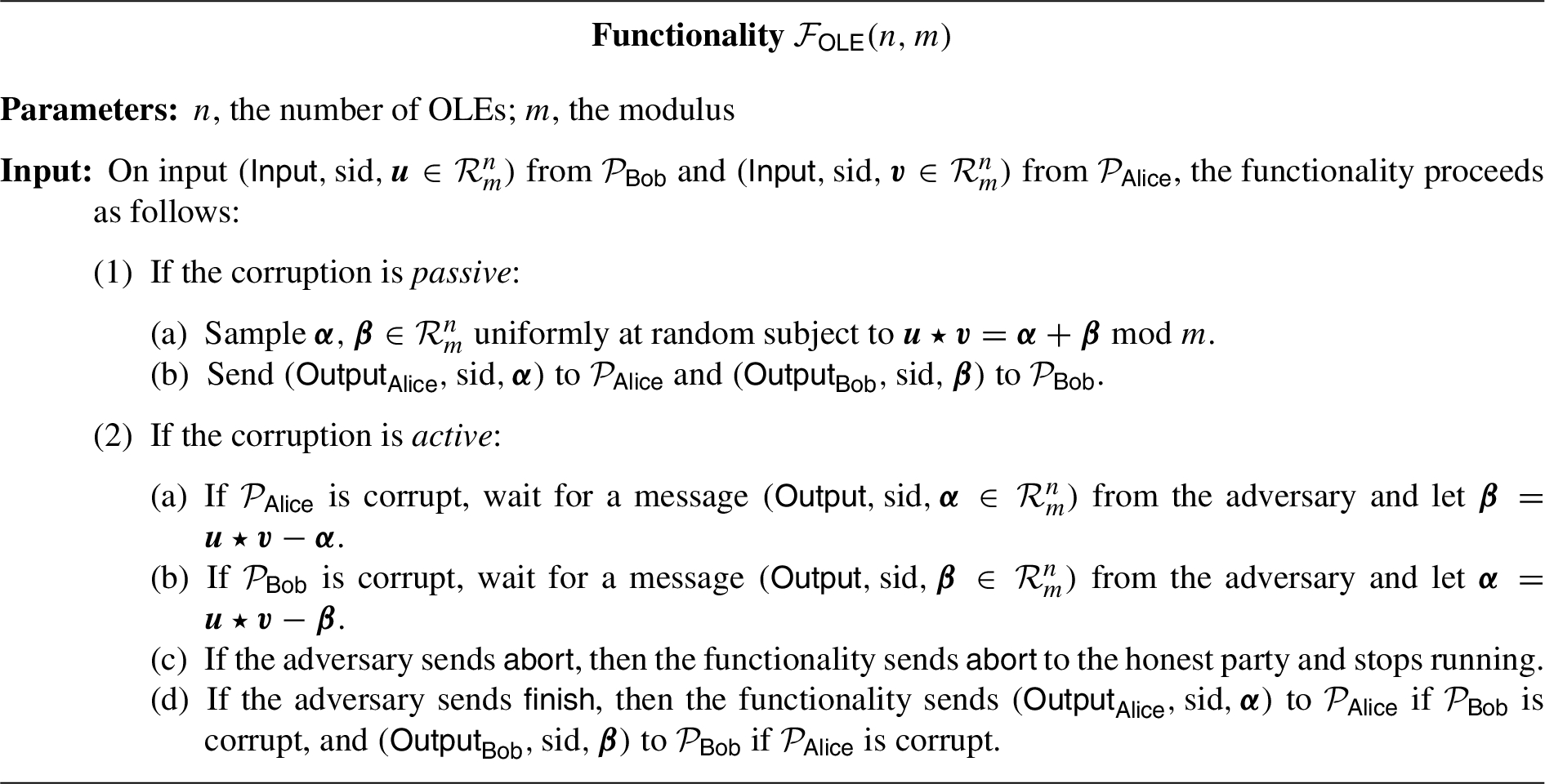
The functionality we implement in this work is oblivious linear evaluation (OLE), which, in a nutshell, consists of producing an additive sharing of a multiplication. A bit more precisely, $P_{Alice}$ and $P_{Bob}$ have each one secret input $v \in R_{m}$ and $u \in R_{m}$ , respectively, and their goal is to get additive random shares of the product $u \cdot v$ . The formal description of the functionality appears in Fig. 1.

Note that our OLE functionality produces several OLE instances simultaneously, and we write $α ⋆ β$ to denote the component-wise product of the vectors $α$ , $β$ .

Fig. 1.

Oblivious linear evaluation functionality.

2.5. SIMD for lattice-based primitives

The OLE functionality above produces OLEs over the ring $R_{m}$ , however, in practice, we wish to produce OLEs over $Z_{m}$ . To do this, we exploit plaintext packing techniques used in homomorphic encryption [49] based on the Chinese remainder theorem. We choose $m = 1 mod (2 N)$ such that the polynomial $X^{N} + 1$ splits completely into a product of linear factors modulo m. This implies that $R_{m}$ is isomorphic to N copies of $Z_{m}$ , so a single OLE over the ring $R_{m}$ can be directly used to obtain a batch of N OLEs over $Z_{m}$ . The isomorphism can be efficiently computed using fast Fourier transform techniques. Therefore, with a single call to our OLE functionality in Fig. 1, we can easily produce a batch of $N \cdot n$ OLEs over $Z_{m}$ .

2.6. Commitments and zero-knowledge arguments

In this work, in order to achieve active security, we make extensive use of commitments schemes and zero knowledge arguments of knowledge.

Commitment schemes

Consider the tuple $C = (KG, Com, Open)$ with $1^{κ}$ as implicit input. $KG$ is a PPT algorithm which generates a public parameter $pk \in {0, 1}^{poly (κ)}$ . $Com$ is a PPT algorithm which on input $pk$ and a message x outputs c, r. Finally, $Open$ is a deterministic poly-time algorithm which on input $pk$ , x, c, r outputs a bit b.

For an algorithm $A$ let $\begin{matrix} Pr [x \neq x^{'} | \begin{matrix} pk \leftarrow KG () \land (x, x^{'}, r, r^{'}, c) \leftarrow A (pk) \\ \land Open (pk, x, c, r) = 1 \land Open (pk, x^{'}, c, r^{'}) = 1 \end{matrix}] ⩽ negl (κ) \end{matrix}$ then we say that C is computationally binding if $A$ is a PPT algorithm and C is statistically binding if $A$ is computationally unbounded.

Furthermore, for an algorithm $A$ if $\begin{matrix} | Pr [i = A (pk, c) | \begin{matrix} pk \leftarrow KG () \land (x_{0}, x_{1}) \leftarrow A (pk) \\ \land i \leftarrow {0, 1} \land (c, r) \leftarrow Com (pk, x_{i}) \end{matrix}] - \frac{1}{2} | ⩽ negl (κ) \end{matrix}$ then we say that the commitment scheme is statistically hiding if $A$ is computationally unbounded or computationally hiding if $A$ is a PPT algorithm.

A commitment scheme is additively homomorphic if for two commitments $(c_{1}, r_{1}) \leftarrow {Com}_{pk} (x_{1})$ , $(c_{2}, r_{2}) \leftarrow {Com}_{pk} (x_{2})$ as well as a constant c, it holds that $Open (pk, c_{1} + c_{2}, x_{1} + x_{2}, r_{1} + r_{2}) = 1$ as well as there exists a polynomial-time algorithm $D$ such that $Open (pk, D (pk, c_{1}, c), x_{1} + c, r_{1}) = 1$ .

In this work we mainly use two different commitment schemes, namely the somewhat additively homomorphic commitment scheme of Baum et al. [8] (denoted as $C = (KG, Com, Open)$ ) as well as a compressing statistically secure commitment scheme $C_{aux} = ({KG}_{aux}, {KG}_{aux}, {Open}_{aux})$ . One can easily instantiate $C_{aux}$ either using the Random Oracle or [27]. The scheme of [8] is only somewhat homomorphic, meaning that it only supports a limited number of addition of commitments due to the growth of r. More details on the used commitment scheme can be found in Section 2.7 below.

Zero-knowledge arguments of knowledge (ZKA)

Let $R$ be an NP relation. For $(p p, x, w) \in R$ we call $p p$ the public parameter, x the statement and w the witness. A Zero-Knowledge Proof of Knowledge for $R$ is an interactive protocol Π between a PPT prover $P$ and a PPT verifier $V$ with the following three properties: Completeness:

If $P$ with input $p p$ , x, w and $V$ with input $p p$ , x follow the protocol honestly, then $V$ outputs 0 only with negligible probability.

Soundness:

The interactive protocol Π is called knowledge-sound with knowledge error ε if for all deterministic polynomial-time algorithms4

⁴
The term “argument of knowledge”, in contrast to “proof of knowledge”, relates to the setting in which soundness is only guaranteed against a polynomially bounded prover.

P^{*}

with input

p p

, x that convince an honest verifier with probability at least ε there exists an expected polynomial-time algorithm

E

which, given black-box access to

P^{*}

, outputs

w^{'}

such that

(p p, x, w^{'}) \in R

except with probability

⩽ ε

Honest-Verifier Zero-Knowledge:

There exists a PPT algorithm $S$ called the simulator whose output distribution on input $p p$ , x and interacting with a PPT algorithm $V^{*}$ is indistinguishable of a transcript of Π run by $P$ , $V^{*}$ .

The actual zero-knowledge arguments that are used with respect to the commitment scheme C can be found in Section 2.7 below.

2.7. Instantiating (somewhat homomorphic) commitments

After having introduced the formal definitions for commitment schemes and zero-knowledge proofs in Section 2.6 we will now recap an implementation which we use in our construction, namely the somewhat homomorphic commitment scheme of Baum et al. [8] and its accompanying zero-knowledge proofs.

A specific property of the scheme of [8] is that it allows “relaxed openings”, meaning that an opening of a commitment $com$ does not just consist of the message x and randomness r but also some additional factor f. The guarantee is then that the scheme is binding as long as it is hard to come up with two $(x, r, f)$ and $(x, r^{'}, f^{'})$ that open the same commitment $com$ . In order to define f properly let $C = {c \in R_{q} ∣ ‖ c ‖_{\infty} = 1 \land ‖ c ‖_{1} = κ}$ as well as $\overline{C} = {c - c^{'} ∣ c \neq c^{'} \in C}$ . [43] showed under which conditions all elements of $C$ , $\overline{C}$ are invertible.

Somewhat homomorphic commitments

The commitment scheme of [8] consists of the following algorithms: $KG$ :

Given $R_{q}$ , N, k, n, β, $σ_{Com}$ sample $A_{1}^{'} \leftarrow R_{q}^{n \times (k - n)}$ as well as $a_{2}^{'} \leftarrow R_{q}^{k - n - 1}$ . Set $A_{1} = [\begin{matrix} I_{n} & A_{1}^{'} \end{matrix}]$ and $a_{2} = [\begin{matrix} 0^{n} & 1 & a_{2}^{'} \end{matrix}]$ and output $pk = (R_{q}, N, k, n, β, A_{1}, a_{2})$ .

Com

On input a valid public key $pk$ and a value $x \in R_{q}$ sample $r \leftarrow S_{β}^{k}$ , compute $\begin{matrix} com = [\begin{matrix} {com}_{1} \\ {com}_{2} \end{matrix}] = [\begin{matrix} A_{1} \\ a_{2} \end{matrix}] \times r + [\begin{matrix} 0^{n} \\ x \end{matrix}] \end{matrix}$ and output $(com, r)$ .

Open

On input a valid public key $pk$ and $com = [\begin{matrix} {com}_{1} \\ {com}_{2} \end{matrix}] \in R_{q}^{n + 1}$ , $x \in R_{q}$ , $r \in R_{q}^{k}$ as well as $f \in \overline{C}$ output 1 iff $\begin{matrix} f \cdot [\begin{matrix} {com}_{1} \\ {com}_{2} \end{matrix}] = [\begin{matrix} A_{1} \\ a_{2} \end{matrix}] \times r + f \cdot [\begin{matrix} 0^{n} \\ x \end{matrix}] and \forall i \in [k] : {‖ r [i] ‖}_{2} ⩽ 4 σ_{Com} \sqrt{N} \end{matrix}$ and 0 otherwise.

[8] showed that their construction is binding under the

{MSIS}_{n, k, 16 σ_{Com} κ N}

assumption and hiding under the

{MLWE}_{n + 1, k, β}

assumption.

It can directly be seen that the commitment scheme is somewhat homomorphic:

If $com = [\begin{matrix} {com}_{1} \\ {com}_{2} \end{matrix}]$ is a commitment that can be opened as $(x, r, f)$ then for a public $x^{'} \in R_{q}$ the commitment ${com}^{'} = [\begin{matrix} {com}_{1} \\ {com}_{2} + x^{'} \end{matrix}]$ can be opened as $(x + x^{'}, r, f)$ .

For h commitments ${com}^{i} = [\begin{matrix} {com}_{1}^{i} \\ {com}_{2}^{i} \end{matrix}]$ with openings $(x^{i}, r^{i}, f)$ we have that $com = [\begin{matrix} \sum_{i \in [h]} {com}_{1}^{i} \\ \sum_{i \in [h]} {com}_{2}^{i} \end{matrix}]$ has opening $(\sum_{i \in [h]} x^{i}, \sum_{i \in [h]} r^{i}, f)$ if $\sum_{i \in [h]} r^{i}$ still fulfills the bound of $Open$ .

In comparison to fully linearly homomorphic commitments it is not possible to generate a commitment

{com}^{'}

from

com

with opening x such that

{com}^{'}

opens to

α \cdot x

for a public α without losing the binding property. Instead, one has to use a zero-knowledge proof to show such a relation. Below we will describe both the standard proof of knowledge for the commitment scheme as well as the proof of linear relation.

2.8. Zero-knowledge proof of opening

The commitment scheme of [8] comes with a highly efficient proof of knowledge and other efficient proofs. The disadvantage of this class of proofs is that soundness does not reduce to a standard opening $(x, r, 1)$ but instead will extract $(x, r, f)$ with $f \in \overline{C}$ . These “extended openings” are never generated by an honest party but possibly by an adversary and are not sufficient in our application. $\begin{matrix} R_{PoK} = \{(p p, u, w) = (\begin{matrix} (R, N, q, pk, σ_{Com}), \\ com, (x, r) \end{matrix}) | \begin{matrix} (x, r) \in R_{q} \times R_{q}^{k} \\ \land {Open}_{pk} (com, x, r, 1) = 1 \end{matrix}\} \end{matrix}$

Instead, we use a “standard” proof of knowledge for a commitment which follows the standard Fiat-Shamir with Aborts signature. The algorithm can be found in Fig. 2.

Fig. 2.

Zero knowledge argument for opening $R_{PoK}$ .

Lemma 4.

Let $M > 1$ and $σ_{Com} ⩾ 12 / ln M \sqrt{β N k}$ as well as $ℓ > κ$ . The algorithm from Fig. 2 is a zero-knowledge argument of knowledge that is complete with probability $1 / M$ , computationally sound and statistically honest-verifier zero knowledge.

Observe that this argument has a much higher communication complexity (by a factor κ) than the optimized AoK of [8] for this commitment scheme, but it has the aforementioned advantage of being more “exact”. Furthermore, in the overall work we will only use it once.

2.9. Zero-knowledge proof of linear relation

Fig. 3.

Zero knowledge argument for linear relation $R_{Lin}$ .

Based on [8] one can easily prove a linear dependency $α \in R_{q}$ between the openings of two commitments. Consider the relation $\begin{matrix} R_{Lin} = \{(p p, u, w) = (\begin{matrix} (R, N, q, pk, σ_{Com}, n, α), \\ {{com}_{i}, {com}_{i}^{'}}_{i \in [n]}, \\ ({x_{i}, r_{i}, r_{i}^{'}, f_{i}}_{i \in [n]}) \end{matrix}) | \begin{matrix} \forall i \in [n] : \\ (x_{i}, r_{i}, r_{i}^{'}, f_{i}) \in R_{q} \times R_{q}^{k} \times R^{k} \times \overline{D} \\ \land {Open}_{pk} ({com}_{i}, x_{i}, r_{i}, f_{i}) = 1 \\ \land {Open}_{pk} ({com}_{i}^{'}, α [i] x_{i}, r_{i}^{'}, f_{i}) = 1 \end{matrix}\} \end{matrix}$

One can use the zero-knowledge proof as outlined in Fig. 3 to prove $R_{Lin}$ , meaning that each of the n commitments ${com}_{i}^{'}$ has an opening that is $α [i]$ away from the opening of ${com}_{i}$ .

Lemma 5.

Let $M > 1$ and $σ_{Com} ⩾ 12 / ln M \sqrt{κ β N k n}$ . The algorithm from Fig. 3 is a zero-knowledge argument of knowledge that is complete with probability $1 / M^{2}$ , computationally sound and statistically honest-verifier zero knowledge.

Proof.

The proof follows as a generalization of the linearity-proof for two commitments of [8]. The only difference is that we adjusted the size of $σ_{Com}$ to allow a rejection-sampling for the whole vector $z_{i}$ , $z_{i}^{'}$ at once, which leads to a slightly worse bound on the extracted openings. □

One important property of the protocol is that the extracted opening for both ${com}_{i}$ , ${com}_{i}^{'}$ will have the same value f for both commitments.

3. OLE from PKI setup

Fig. 4.

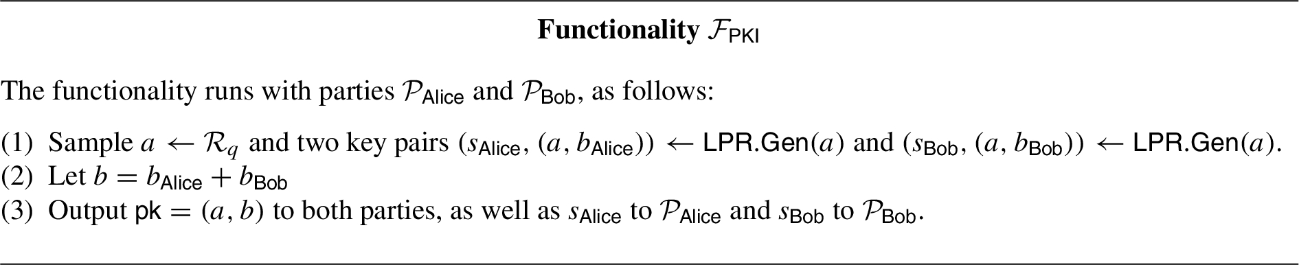
PKI setup functionality.

Fig. 5.

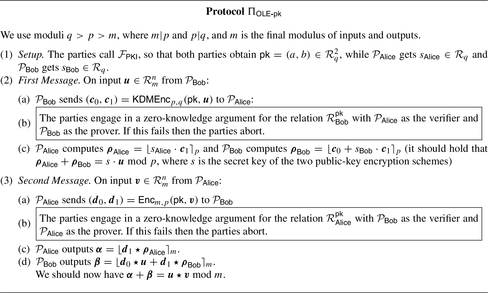
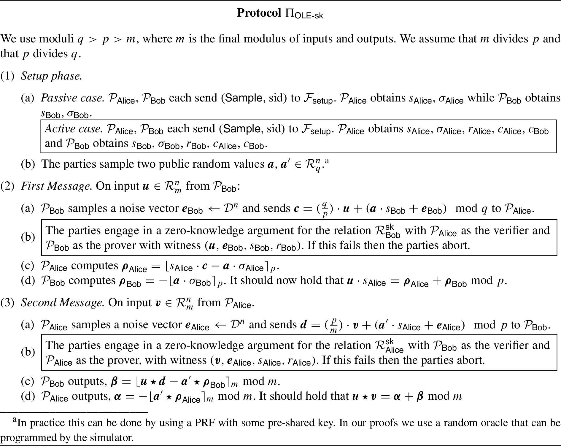
Actively secure OLE protocol from a PKI setup. The passively secure version of the protocol is obtained by removing the framed steps.

In this section we present our first OLE construction, which is particularly simple and efficient. Furthermore, the only setup required is a correlated form of public key infrastructure for the LPR encryption scheme from Section 2.3 in which $P_{Alice}$ and $P_{Bob}$ have each a secret/public key pair for the LPR scheme, where the $a \in R_{q}$ component of the public key is the same for both. This can be seen as a PKI setup in which the public keys are derived using some public randomness. The precise functionality $F_{PKI}$ is given in Fig. 4.

Our protocol, $Π_{OLE - pk}$ , can be found in Fig. 5. The passively secure version $Π_{OLE - pk}^{passive}$ is obtained from the active one by removing the zero knowledge arguments, whose steps are framed in the description of the protocol. To provide a high level idea of our construction, we first recall the main techniques from the homomorphic secret-sharing scheme of Boyle et al. [20]. Suppose two parties have additive secret shares of a RLWE secret key $s \in R_{q}$ , and are also given secret shares modulo q of x, $x \cdot s$ and a public ciphertext $c_{y} = (c_{0}, c_{1}) = Enc (pk, y)$ , for some messages x, y. Boyle et al. observed that if each party locally decrypts $c_{y}$ using its shares, denoted $[x]$ , $[x \cdot s]$ , we have: $\begin{matrix} [x] \cdot c_{0} + [x \cdot s] \cdot c_{1} = [x \cdot (c_{0} + c_{1} \cdot s)] \approx [(q / p) \cdot x \cdot y] . \end{matrix}$ Applying the rounding operation from decryption on the above shares then gives exact additive shares of $x \cdot y$ , provided the error is much smaller than $q / p$ .

To create the initial shares of x and $x \cdot s$ , it is enough to start with shares of s and ciphertexts encrypting x, $x \cdot s$ , since each ciphertext can then be locally decrypted to obtain shares of these values. Boyle et al. also described a variant which removes the need for encryptions of $x \cdot s$ , but at the cost of an additional setup assumption involving shares of $s^{2}$ .

Our OLE protocol from this section builds upon this blueprint, with some optimizations. First, we observe that in the two-party OLE setting, it is not necessary to give out $Enc (pk, x)$ to obtain shares of x, since one of the parties always knows x so they can simply choose these shares to be x and 0. (This is in contrast to the homomorphic secret-sharing setting, where the evaluating parties may be a set of servers who did not provide inputs.) Since we only do one multiplication, it’s therefore enough to give out the two ciphertexts $c_{x} = Enc (pk, x \cdot s)$ and $c_{y} = Enc (pk, y)$ , compared with four ciphertexts used in the HSS scheme from [20]. Since both ciphertexts can be easily generated from the public-key setup, this leads to a very simple protocol where each party (in parallel) sends a single message that is either an encryption of its input, or its input times s.

As an additional optimization, we show that the second ciphertext encrypting y can be defined at a smaller modulus p instead of q, since we only care about obtaining the result modulo $m < p$ , which saves further on bandwidth.5

⁵

This optimization is possible since we skip the “modulus lifting” step from [20], which is only needed when doing several repeated multiplications.

The protocol described above is passively secure, but an active adversary can break the security of this construction by sending incorrectly-formed ciphertexts. Due to our simple communication pattern this turns out to be the only potential source of attack, which we rule out by having the parties prove, in zero knowledge, that their ciphertexts are correctly formed.

3.1. Passive security

We now proceed to the security proof of our protocol $Π_{OLE - pk}^{passive}$ , which consists of protocol $Π_{OLE - pk}$ in Fig. 5 without the zero knowledge arguments framed in the protocol description.

Our proof requires that a random element of $R_{q}$ is invertible with high probability. As we will see, this technicality allows the simulator to “solve equations”, matching real and ideal views. For our choice of parameters this is always the case, and for this we make use of the following lemma.

Lemma 6.
Let $q = \prod_{i = 1}^{k} p_{i}$ , where each $p_{i}$ is an ℓ-bit prime. If the polynomial $f (x) \in Z_{q} [x]$ of degree N used to define $R_{q}$ splits completely mod $p_{i}$ as $f (x) = \prod_{j = 1}^{N} f_{i j} (x) mod p_{i}$ , where each $f_{i j} (x)$ is linear, then the probability that a uniformly random element from $R_{q}$ is not invertible is upper bounded by $\frac{N \cdot k}{2^{ℓ}}$ .
Proof.
The conditions in the lemma imply that $R_{q} ≅ {(F_{p_{1}})}^{N} \times \dots \times {(F_{p_{k}})}^{N}$ , and an element in $R_{q}$ is not invertible if and only if one of its components in $F_{p_{i}}$ from the decomposition above is zero. This happens with probability $1 / 2^{ℓ}$ for each component, so by the union bound, the probability that at least one of these components is zero is bounded by $N \cdot k \cdot 2^{- ℓ}$ . □

Given the above, the probability that at least one component of a vector in $R_{q}^{n}$ is not invertible is upper bounded by $n \cdot N \cdot k \cdot 2^{- ℓ}$ . For all our parameter sets in Section 6, this quantity is below $2^{- λ}$ for $λ \approx 36$ , which is good enough for our purposes since we need it only as an artefact for the proof and it does not lead to any concrete attack or leakage.6
⁶
This restriction can be easily overcome by modifying the definition of security against passive adversaries, allowing the adversary to choose its output. However, we prefer to stick to more standard security definitions.

We also use invertibility to argue correctness of the protocol: it is necessary in the simulation argument to find solutions for a certain equation. If this probability is not good enough for a certain application, the parties could use a PRF to rerandomize their shares so that this lemma can be applied without invertibility. However, in order to keep our exposition simple we do not discuss such extension.

Another simple but useful lemma for our construction is the following.
Lemma 7.
Assume that $p | q$ . Given $y \in R_{p}$ , the set of $x \in R_{q}$ such that ${y = ⌊ x ⌉}_{p}$ is given by $x = (\frac{q}{p}) \cdot y + e$ for $e \in Z \cap (- q / 2 p, q / 2 p]$ . In particular, the mapping $R_{q} \to R_{p}$ given by ${x \mapsto ⌊ x ⌉}_{p}$ is a surjective regular mapping, meaning that every element in the codomain has an equal number of preimages.

Finally, we have the following proposition, concerning correctness of our construction. It follows as a corollary of Proposition 2 by setting the soundness slack parameter τ to be 1, so we defer the proof to that section.
Proposition 1.
Assume that $5 \cdot 2^{κ + 1} \cdot n \cdot m^{2} \cdot N^{3} \cdot B_{err} \cdot B_{sk} ⩽ p ⩽ \frac{q}{5 \cdot 2^{κ + 1} \cdot n \cdot N^{2} \cdot B_{err} \cdot B_{sk}}$ . Let $u, v \in R_{m}^{n}$ be the inputs to Protocol $Π_{OLE - pk}^{passive}$ , and let $α, β \in R_{m}^{n}$ be the outputs. Then, with probability at least $1 - 2^{- κ}$ , $u ⋆ v = α + β$ .

With these tools at hand we proceed with the main result from this section. Theorem 2.
Assume that $5 \cdot 2^{κ + 1} \cdot n \cdot m^{2} \cdot N^{3} \cdot B_{err} \cdot B_{sk} ⩽ p ⩽ \frac{q}{5 \cdot 2^{κ + 1} \cdot n \cdot N^{2} \cdot B_{err} \cdot B_{sk}}$ . Then protocol $Π_{OLE - pk}^{passive}$ , which consists of protocol $Π_{OLE - pk}$ without the underlined steps, realizes functionality $F_{OLE}$ in the $F_{PKI}$ -hybrid model under the RLWE assumption.
Proof.
Let us consider first the case in which $P_{Bob}$ is passively corrupt. The transcript of the computation for an environment $Z$ that corrupts $P_{Bob}$ consists of the inputs $(u, v)$ , the values from the setup phase $(s_{Bob}, b_{Bob}, a)$ , the intermediate messages $(d_{0}, d_{1})$ and the outputs $(α, β)$ . Our goal is to show the existence of a simulator $S$ that, on input $(u, β)$ , can simulate the transcript above so that it is indistinguishable from a real execution.

The simulator proceeds as follows. It emulates the setup phase by sampling a, $s_{Alice}$ , $s_{Bob}$ , $b_{Alice}$ , $b_{Bob}$ as in the real execution, and it sets $(c_{0}, c_{1}) = KDMEnc (pk, u)$ . Then it lets ${ρ_{Bob} = ⌊ c_{0} + s_{Bob} \cdot c_{1} ⌉}_{p}$ , samples $d_{0} \leftarrow R_{p}^{n}$ and samples a uniformly random $d_{1} \in R_{p}^{n}$ subject to ${β = ⌊ d_{0} ⋆ u + d_{1} ⋆ ρ_{Bob} ⌉}_{m}$ . To find a suitable $d_{1}$ , we first apply Lemma 7 to obtain a random preimage $y$ of $β$ under rounding. We then choose $d_{1}$ by finding $x$ such that $y = d_{0} ⋆ u + x ⋆ ρ_{Bob} mod q$ . This can be done since all entries in $ρ_{Bob}$ are invertible with probability at least $2^{- λ}$ .

To argue that the distribution of the values outputted by $S$ are computationally indistinguishable from those in the real execution, we consider a hybrid distribution as follows: Hybrid $H_{1}$ .
The execution is as in the ideal world, but the functionality $F_{OLE}$ is modified so that $S$ can choose the output $β$ . This way, instead of getting $β$ and then sampling $(d_{0}, d_{1})$ so that ${β = ⌊ d_{0} ⋆ u + d_{1} ⋆ ρ_{Bob} ⌉}_{m}$ , the simulator samples $(d_{0}, d_{1})$ completely at random and then defines ${β : = ⌊ d_{0} ⋆ u + d_{1} ⋆ ρ_{Bob} ⌉}_{m}$ , and sends this to the functionality $F_{OLE}$ .
Hybrid $H_{2}$ .
The execution is as in the hybrid $H_{1}$ , but instead of sampling $(d_{0}, d_{1})$ uniformly at random, these are obtained as encryptions of the input $v$ from $Z$ for the real-world $P_{Alice}$ .
Claim 1.
The ideal execution and the hybrid $H_{1}$ are statistically indistinguishable.

This follows from Lemma 7 and from the invertibility of all the entries in $ρ_{Bob}$ , since these imply that the function ${⌊ \cdot ⌉}_{m}$ is a regular function and as a result one can either sample its output $β$ and then sample a uniform input $d_{0} ⋆ u + d_{1} ⋆ ρ_{Bob}$ that maps to $β$ , which corresponds to the ideal world, or one can sample the input uniformly first and then compute the output, which corresponds to the hybrid $H_{1}$ . Claim 2.
The hybrids $H_{1}$ and $H_{2}$ are computationally indistinguishable.

This is based on the security of the RLWE problem. We define an adversary $A^{'}$ playing the CPA game for the LPR encryption scheme, which is defined as follows: $A^{'}$ receives a public key $pk$ from the challenger and it then replies with some message $v$ , the challenger then tosses an internal coin and returns $(d_{0}, d_{1})$ to $A^{'}$ where the pair is either an encryption of $v$ or a uniformly random pair. The goal of $A^{'}$ is to guess the internal bit from the challenger.

Our adversary $A^{'}$ proceeds by playing an honest $P_{Alice}$ and the simulator $S$ above, using the public key received from the challenger. Upon receiving $P_{Alice}$ ’s input $v$ from $Z$ , $A^{'}$ sends $v$ to the challenger and receives $(d_{0}^{}, d_{1}^{})$ $A^{'}$ plays the protocol, but uses $(d_{0}^{}, d_{1}^{})$ in place of $(d_{0}, d_{1})$ .

We notice the following. If $(d_{0}^{}, d_{1}^{})$ is an encryption of $v$ , then the execution corresponds to the hybrid $H_{2}$ . On the other hand, if $(d_{0}^{}, d_{1}^{})$ is uniform, then this is precisely the hybrid $H_{1}$ . Therefore, the advatange of $Z$ is upper bounded by the advantage of $A^{'}$ , which is negligible from the security of the LPR encryption scheme. Claim 3.
The real execution and the hybrid $H_{2}$ are statistically indistinguishable.

Our first observation is that the intermediate values from the setup phase $(s_{Bob}, b_{Bob}, a)$ and the intermediate messages $(d_{0}, d_{1})$ follow the exact same distribution in both executions, so the only potential distinguishing point is the output pair $(α, β)$ : In the hybrid $H_{2}$ it holds that ${β = ⌊ d_{0} ⋆ u + d_{1} ⋆ ρ_{Bob} ⌉}_{m}$ and $α = u ⋆ v - β$ , whereas in the real world $α$ is defined as ${α = ⌊ d_{1} \cdot ρ_{Alice} ⌉}_{m}$ . It suffices to show then that $u ⋆ v = α + β$ holds in the real world as well. This holds with probability at least $1 - 2^{- κ}$ , as shown in Proposition 1.

This concludes the proof of the claim, and with it, the proof of the theorem. □

3.2. Active security

As we saw in the previous section, the correctness of our construction relies on the different terms involved having a certain bound: The input $u$ must be smaller than m, the noise terms used for the encryption have to be upper bounded by $B_{err}$ , and the randomness $w$ and $w^{'}$ used for the encryption must be less than $B_{sk}$ . An actively corrupted party who chooses randomness outside these bounds can easily distinguish between the real and ideal executions.

To achieve active security, each party proves in zero-knowledge that the ciphertexts they send are correctly formed. We begin by analyzing the case of a corrupt $P_{Bob}$ . Consider the message from $P_{Bob}$ , which consists of a batch of ciphertexts $\begin{matrix} (c_{0}, c_{1}) = (b \cdot w + e_{0}, (q / p) \cdot u - a \cdot w + e_{1}) \end{matrix}$

Rewriting this, $P_{Bob}$ has to prove knowledge of vectors (over $R_{q}$ ) $w$ , $u$ , $e_{0}$ , $e_{1}$ satisfying $\begin{matrix} (3) & \underset{A}{\underset{︸}{(\begin{matrix} b & 1 & 0 & 0 \\ - a & 0 & 1 & q / p \end{matrix})}} \cdot \underset{S}{\underset{︸}{{(\begin{matrix} w & e_{0} & e_{1} & u \end{matrix})}^{⊤}}} = \underset{T}{\underset{︸}{(\begin{matrix} c_{0} \\ c_{1} \end{matrix})}} \end{matrix}$ and $‖ w ‖_{\infty} ⩽ B_{sk}$ , $‖ u ‖_{\infty} ⩽ m$ , $‖ e_{0} ‖_{\infty} ⩽ B_{err}$ and $‖ e_{1} ‖_{\infty} ⩽ B_{err}$ . This can be written in matrix form as follows $\begin{matrix} R_{Bob}^{pk} = \{(p p, u, w) = ((R, q, n, β, A), T, S) | \begin{matrix} (A, S, T) \in R_{q}^{2 \times 4} \times R^{4 \times n} \times R_{q}^{2 \times n} \\ \land A S = T \land ‖ s_{i} ‖_{\infty} ⩽ β_{i} \end{matrix}\} \end{matrix}$ where $s_{i}$ is the i-th row of $S$ and the bound vector is $β = (B_{sk}, B_{err}, B_{err}, B_{msg})$ . Such type of statements can be proven efficiently using the amortized proof from [5], as we discuss more thoroughly in Section 5.

We can similarly define a relation for the message $(d_{0}, d_{1})$ that $P_{Alice}$ sends, and we call this relation $R_{Alice}^{pk}$ . We note however that in the proof of Theorem 2 we did not actually use any bound on the message $v$ , so we may exclude the bound $‖ v ‖_{\infty} ⩽ m$ from this relation.

For the rest of this section we assume the existence of zero knowledge arguments of knowledge for the relations $R_{Alice}^{pk}$ and $R_{Bob}^{pk}$ . As mentioned above, we show how to construct these in Section 5.1. Note that when proving knowledge of the relation $R_{Bob}^{pk}$ or $R_{Alice}^{pk}$ above, if the prover is malicious then our proof actually only guarantees that $‖ s_{i} ‖_{2} ⩽ τ \cdot β_{i}$ , where τ is the soundness slack parameter of the zero knowledge argument. We therefore need to choose our parameters with respect to the larger bounds, to ensure correctness of the protocol.

We begin with the following proposition, which shows that, under an appropriate choice of parameters, our protocol guarantees correctness.

Proposition 2.
Assume that $5 \cdot 2^{κ + 1} \cdot n \cdot τ \cdot m^{2} \cdot N^{3} \cdot B_{err} \cdot B_{sk} ⩽ p ⩽ \frac{q}{5 \cdot 2^{κ + 1} \cdot n \cdot τ \cdot N^{2} \cdot B_{err} \cdot B_{sk}}$ . Let $u, v \in R_{m}^{n}$ be the inputs to Protocol $Π_{OLE - pk}$ , and let $α, β \in R_{m}^{n}$ be the outputs. Assume that the relations $R_{Alice}^{pk}$ and $R_{Bob}^{pk}$ defined in Section 3.2 hold, but that at most one of them has slack parameter τ.7
⁷
That is, the bounds in one of the two relations have an extra factor of τ. This corresponds to what can be guaranteed for a corrupt party via the zero knowledge argument.

Then, with probability at least $1 - 2^{- κ}$ , $u ⋆ v = α + β$ .
Proof.
Let us begin by writing the individual public keys as $b_{Bob} = a \cdot s_{Bob} + e_{Bob}$ and $b_{Alice} = a \cdot s_{Alice} + e_{Alice}$ , and let $b = b_{Bob} + b_{Alice}$ and $s = s_{Bob} + s_{Alice}$ , so $b = a \cdot s + e$ where $e = e_{Alice} + e_{Bob}$ . Assuming that b is honestly generated, it holds that $‖ s_{Alice} ‖_{\infty}, ‖ s_{Bob} ‖_{\infty} ⩽ B_{sk}$ and similarly $‖ e_{Alice} ‖_{\infty}, ‖ e_{Bob} ‖_{\infty} ⩽ B_{err}$ . Therefore, $‖ s ‖_{\infty} ⩽ 2 \cdot B_{sk}$ and $‖ e ‖_{\infty} ⩽ 2 \cdot B_{err}$ . We also write $(c_{0}, c_{1}) = (b \cdot w + e_{0}, (q / p) \cdot u - a \cdot w + e_{1})$ and $(d_{0}, d_{1}) = (b \cdot w^{'} + e_{0}^{'} + (p / m) \cdot v, - a \cdot w^{'} + e_{1}^{'})$ . It follows then that $\begin{array}{l} c_{0} + s \cdot c_{1} & = b \cdot w + e_{0} + (q / p) \cdot s \cdot u - s \cdot a \cdot w + s \cdot e_{1} \\ = (b - s \cdot a) \cdot w + e_{0} + (q / p) \cdot s \cdot u + s \cdot e_{1} \\ = (q / p) \cdot s \cdot u + \underset{e}{\underset{︸}{(e_{0} + e \cdot w + s \cdot e_{1})}} mod q . \end{array}$ By recalling that $s = s_{Alice} + s_{Bob}$ , we can write this as $c_{0} + s_{Bob} \cdot c_{1} = (q / p) \cdot s \cdot u + (- s_{Alice} \cdot c_{1} + e) mod q$ . Rounding this equation modulo p, we see that $\begin{matrix} {{⌊ c_{0} + s_{Bob} \cdot c_{1} ⌉}_{p} = s \cdot u + ⌊ - s_{Alice} \cdot c_{1} + e ⌉}_{p} mod p . \end{matrix}$

From $R_{Bob}^{pk}$ we know that $‖ w ‖_{\infty} ⩽ τ \cdot B_{sk}$ and that $‖ e_{i} ‖_{\infty}, ‖ e_{i}^{'} ‖_{\infty}$ for $i = 1, 2$ are upper bounded by $τ \cdot B_{err}$ . By a well-known bound on products of elements in $R_{q}$ , it holds that $‖ e \cdot w ‖_{\infty} ⩽ 2 N τ B_{sk} B_{err}$ as well as $‖ s \cdot e_{1} ‖_{\infty} ⩽ 2 N τ B_{sk} B_{err}$ . Therefore we can upper-bound $‖ e ‖_{\infty} ⩽ 5 τ N B_{err} B_{sk} ⩽ \frac{q}{2^{κ + 1} \cdot n \cdot p \cdot N}$ . Also, since $s_{Alice} \cdot c_{1}$ is close to uniform, it follows from Lemma 1 that ${{{⌊ - s_{Alice} \cdot c_{1} + e ⌉}_{p} = ⌊ - s_{Alice} \cdot c_{1} ⌉}_{p} = - ⌊ s_{Alice} \cdot c_{1} ⌉}_{p}$ with probability at least $1 - 2^{- κ}$ . From this we conclude that $ρ_{Alice} + ρ_{Bob} = s \cdot u mod p$ with high probability.

Now, we can perform a similar analysis for $(d_{0}, d_{1})$ by writing $\begin{array}{l} d_{0} + s \cdot d_{1} & = b \cdot w^{'} + e_{0}^{'} + (p / m) \cdot v - a \cdot s \cdot w^{'} + s \cdot e_{1}^{'} \\ = (b - s \cdot a) \cdot w^{'} + e_{0}^{'} + (q / p) \cdot v + s \cdot e_{1}^{'} \\ = (p / m) \cdot v + \underset{e^{'}}{\underset{︸}{(e_{0}^{'} + e \cdot w^{'} + s \cdot e_{1}^{'})}} mod p . \end{array}$ We can multiply both sides by $u$ to get $d_{0} ⋆ u + (s \cdot u) ⋆ d_{1} = (p / m) \cdot (u ⋆ v) + u ⋆ e^{'} mod p$ , and recalling that $u \cdot s = ρ_{Alice} + ρ_{Bob} mod p$ with high probability we obtain that $\begin{matrix} d_{0} ⋆ u + ρ_{Bob} ⋆ d_{1} = (\frac{p}{m}) \cdot (u ⋆ v) + (- ρ_{Alice} ⋆ d_{1} + u ⋆ e^{'}) mod p . \end{matrix}$

If $R_{Bob}^{pk}$ holds with slack τ and $R_{Alice}^{pk}$ with slack 1, then we know that $‖ u ‖_{\infty} ⩽ τ \cdot m$ , $‖ w^{'} ‖_{\infty} ⩽ B_{sk}$ and $‖ e_{i}^{'} ‖_{\infty} ⩽ B_{err}$ for $i = 1, 2$ , so $‖ e^{'} ‖_{\infty} ⩽ 5 N B_{err} B_{sk}$ . On the other hand, if $R_{Bob}^{pk}$ holds with slack 1 and $R_{Alice}^{pk}$ with slack τ, then we know that $‖ u ‖_{\infty} ⩽ m$ , $‖ w^{'} ‖_{\infty} ⩽ τ \cdot B_{sk}$ and $‖ e_{i}^{'} ‖_{\infty} ⩽ τ \cdot B_{err}$ for $i = 1, 2$ , so $‖ e^{'} ‖_{\infty} ⩽ 5 N τ B_{err} B_{sk}$ . Either case, it holds that $‖ u ⋆ e^{'} ‖_{\infty} ⩽ 5 m τ N^{2} B_{err} B_{sk} ⩽ \frac{p}{2^{κ + 1} \cdot n \cdot m \cdot N}$ . Hence, rounding this equation modulo m, and using Lemma 1, we conclude that $u ⋆ v = α + β mod m$ with probability at least $1 - 2^{- κ}$ , as required. □

With this tool at hand, the security of the actively secure version of our protocol can be proven. Theorem 3.
Assume that $5 \cdot 2^{κ + 1} \cdot n \cdot τ \cdot m^{2} \cdot N^{3} \cdot B_{err} \cdot B_{sk} ⩽ p ⩽ \frac{q}{5 \cdot 2^{κ + 1} \cdot n \cdot τ \cdot N^{2} \cdot B_{err} \cdot B_{sk}}$ . Protocol $Π_{OLE - pk}$ realizes functionality $F_{OLE}$ under the RLWE assumption.
Proof.
We define a simulator $S$ that interacts with the environment $Z$ as follows.

Corrupt Bob. The simulator emulates an honest party $P_{Alice}$ , and it also emulates the PKI resource by sampling $a \leftarrow R_{q}$ and two key pairs $(s_{Alice}, (a, b_{Alice})) \leftarrow Gen (a)$ and $(s_{Bob}, (a, b_{Bob})) \leftarrow Gen (a)$ , and sending the public key $pk = (a, b)$ to both $P_{Alice}$ and $P_{Bob}$ , $s_{Alice}$ to $P_{Alice}$ and $s_{Bob}$ to $P_{Bob}$ . After this setup phase the emulated $P_{Alice}$ receives $(c_{0}, c_{1})$ from $P_{Bob}$ , and she runs the zero knowledge argument for $R_{Bob}^{pk}$ honestly and, if the proof succeeds, $S$ uses the knowledge on the secret key $s = s_{Alice} + s_{Bob}$ to decrypt a message $u$ .

The emulated $P_{Alice}$ computes $(d_{0}, d_{1}) = Enc (pk, 0)$ and sends the input $u$ and output $β$ to the functionality $F_{OLE}$ , where ${β = ⌊ d_{0} ⋆ u + d_{1} ⋆ ρ_{Bob} ⌉}_{m} mod m$ . Then it sends $(d_{0}, d_{1})$ to $P_{Bob}$ and then runs the zero knowledge argument for $R_{Alice}^{pk}$ honestly, which she can do since she knows the witness.

To argue that the real and the ideal world are indistinguishable, it is useful to consider the following hybrid: Hybrid $H$ .
The execution is as in the ideal world, except that the actual input $v$ from real-world $P_{Alice}$ is used to define $(d_{0}, d_{1})$ , and the zero knowledge argument for $R_{Alice}^{pk}$ uses this input.
Claim 4.
The real execution is statistically indistinguishable from the hybrid $H$ .

Begin by noticing that there is no difference between the intermediate messages in these two executions. The only potential difference originates in the input/output relation: in the hybrid it is the case that $α + β = u ⋆ v$ , so we only need to show that this is the case too in the real execution.

To see this, first observe that the extractor $E$ from the ZKA for $R_{Bob}^{pk}$ can interact with $Z$ to obtain a witness for $R_{Bob}^{pk}$ , i.e. $w = (w, e_{0}, e_{1}, u)$ such that $(c_{0}, c_{1}) = (b \cdot w + e_{0}, (q / p) \cdot u - a \cdot w + e_{1})$ with $‖ u ‖_{\infty} ⩽ τ \cdot m$ , $‖ w ‖_{\infty} ⩽ τ \cdot B_{sk}$ , $‖ e_{0} ‖_{\infty} ⩽ τ \cdot B_{err}$ and $‖ e_{1} ‖_{\infty} ⩽ τ \cdot B_{err}$ . What the simulator computes, on the other hand, is $c_{0} + s \cdot c_{1} = (q / p) \cdot s \cdot u + e$ , where $e = e_{0} + e \cdot w + s \cdot e_{1}$ , and then rounds to p. The bounds above imply that $‖ e ‖_{\infty} ⩽ 5 τ N B_{err} B_{sk}$ , which just needs to be below $q / 2 p$ to guarantee correct decryption. This is clearly implied by the bound in the theorem statement.

As a result, the value that the simulator decrypts is exactly the $u$ from the witness. At this point we can apply Proposition 2 with τ being the slack parameter from the ZKA to conclude that $u ⋆ v = α + β$ holds in the real world with probability at least $1 - 2^{- κ}$ . Claim 5.
The hybrid $H$ is computationally indistinguishable from the ideal world.

Here we notice that the only difference between these two scenarios is the message $(d_{0}, d_{1})$ (and its corresponding ZKA). It suffices then to argue that these two are indistinguishable, which intuitively hold because of the security of the encryption scheme and the zero knowledge property of the ZKA for $R_{Alice}^{pk}$ .

In a bit more detail, consider an adversary $A^{'}$ for the following game: $A^{'}$ gets a public key $pk$ and sends $v \in R_{m}^{n}$ to a challenger who samples a bit internally and returns $(d_{0}, d_{1}) = Enc (pk, 0)$ if the bit is 0, and $(d_{0}, d_{1}) = Enc (pk, v)$ if the bit is 1. This is essentially the semantic security of the LPR encryption scheme and its security can be proved based on RLWE [42]. Our adversary $A^{'}$ is defined as follows: it runs a copy of $Z$ internally and interacts with by playing the honest $P_{Alice}$ and the simulator $S$ . $A^{'}$ gets $pk$ from the challenger and uses this for the PKI setup. Notice that $A^{'}$ does not know the secret key s that the challenger used, but it still can give $P_{Bob}$ a uniformly random secret key $s_{Bob}$ , which implicitly defines a secret key $s_{Alice}$ for $P_{Alice}$ (that $A^{'}$ does not know!).

The simulator then receives $v$ from $Z$ and $A^{'}$ passes this value to the challenger, getting back the challenge $(d_{0}, d_{1})$ . $S$ uses this as the second message from $P_{Alice}$ to $P_{Bob}$ . Now, the main issue with the interaction above is that $P_{Alice}$ cannot prove $R_{Alice}^{sk}$ now, since she does not know the witness. To this end, consider the simulator $M$ for the ZKA for $R_{Alice}^{sk}$ . $A^{'}$ has the public parameters and the instance information from the interaction with $Z$ , so it can use $M$ to interact with $Z$ and pass the ZKA. If $Z$ claims the resulting interaction is from the ideal world, then $A^{'}$ outputs 0, and if $Z$ claims the interaction is in the real world then $A^{'}$ outputs 1.

We claim now that the adversary $A^{'}$ above wins the game with an advantage that is negligibly close to the advantage with which $Z$ distinguishes $H$ from the ideal world, which implies that the latter must be negligible, as the original claim stated. To see this, first notice that, for a fixed $(d_{0}, d_{1})$ , $Z$ cannot distinguish between interacting with $M$ and interacting with a prover who knows the witness. This holds by the zero knowledge property of the ZKA. As a result, the advantage of $A^{'}$ is negligibly close to the difference between the probability of $Z$ outputting “ideal world” and the probability of $Z$ outputting “ $H$ ” when the ZKA is computed correctly. Finally, given that the interaction of $Z$ with $A^{'}$ corresponds to either the ideal world (for challenge 0) or the hybrid $H$ (for challenge 1) when the ZKA is computed correctly, we conclude that this difference is precisely the distinguishing advantage of $Z$ , which concludes the proof of the claim and with it the proof of indistinguishability for a corrupt $P_{Bob}$ .

Corrupt Alice (sketch). The proof in this setting is similar to the one considered above and therefore we only provide a sketch. The simulator uses the same idea of encrypting a dummy input $u = 0$ on behalf of the emulated honest $P_{Bob}$ , and running the ZKA for $R_{Bob}^{pk}$ honestly. To prove indistinguishability of the ideal and real worlds, a similar hybrid as above is considered where this message uses the real $u$ .

Proving that the hybrid is indistinguishable from the real world follows along the same lines as above. However, proving that the hybrid is indistinguishable from the ideal world requires a small change, given that now $u$ is not encrypted, but KDM-encrypted. This, fortunately, is not a problem since KDM-encryptions are indistinguishable from proper encryptions, as shown in [20]. □

4. OLE from correlated setup

Ciphertexts in the public key version of the LPR cryptosystem consist of two ring elements. However, in the secret key variant, we can reduce this to one element, since the first element is uniformly random so can be compressed using, for example, a PRG. Given this, a natural way of shaving off a factor of two in the communication complexity of our protocol from Section 3 would be to use secret key encryption instead of public key.

In this section we present an OLE protocol that instantiates precisely this idea. The communication pattern is very similar to the one from Protocol $Π_{OLE - pk}$ , in which there is a setup phase, then $P_{Bob}$ sends an encryption of his input $u$ to $P_{Alice}$ (and proves in zero-knowledge its correctness for the actively secure version), and then $P_{Alice}$ does the same. The challenge, here, is that now, as we are using secret-key encryption to obtain his ciphertext in the first message, there is no way for Bob to encrypt $u$ multiplied by the (combined) secret key.

To make this work, we replace the PKI setup functionality from the previous section with a more specialized setup, where $P_{Bob}$ gets $σ_{Bob} \in R_{q}$ and $P_{Alice}$ gets $σ_{Alice} \in R_{q}$ such that $s_{Alice} \cdot s_{Bob} = σ_{Alice} + σ_{Bob} mod q$ . This can be seen as an OLE itself, where the values being multiplied are small RLWE secret keys; under this interpretation, our protocol can be seen as a form of “OLE extension” protocol. The intuition for why this setup is useful, is that Bob’s secret-key ciphertext can now be distributively “decrypted” using the shares of $s_{Alice} \cdot s_{Bob}$ , which (after rounding) leads to shares of $u \cdot s_{Alice}$ . In the second phase, these shares are then used to “decrypt” Alice’s ciphertext, giving shares of the product $u ⋆ v$ .

Fig. 6.

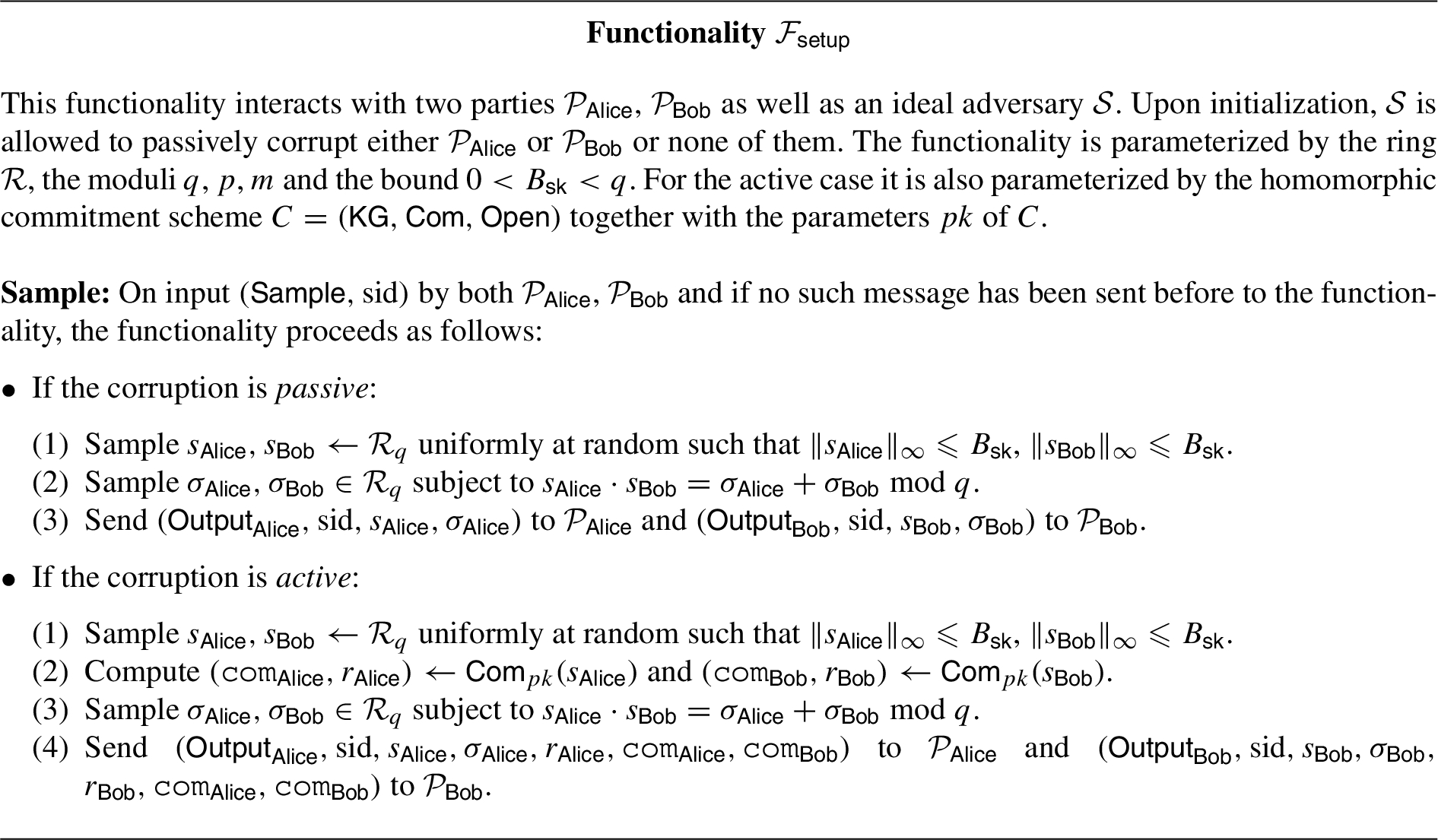
Preprocessing for OLE with passive security.

Fig. 7.

Actively secure OLE protocol based on RLWE. The passively secure version of the protocol is obtained by removing the framed steps.

The setup functionality is described in Fig. 6, where we present both the passive and active versions of the functionality, with the main difference being that in the active setting we must ensure that the corrupt party uses the same secret key for encrypting its input as the secret key distributed in the setup phase. Thus, in this case, when the corrupted party proves in zero knowledge the correctness of its encryption, it also proves that the secret key is the same as in the setup phase. This requires the setup functionality in the active case to output some extra information that allows us to “bind” the key from the setup with the key from the encryption sent, for which we use commitments. We discuss this in more detail when we look at active security in Section 4.2. In Section 4.3, we also discuss how this setup functionality can be implemented in practice.

Our protocol is described in full detail in Fig. 7. As in Section 3, we present the full, actively secure version, but outline in a box those steps that are only necessary for active security.

4.1. Passive security

The following proposition states that our construction satisfies correctness when the parties are honest, and follows from Proposition 4 in Section 4.2, which analyzes the case where the bounds satisfied by the values from one of the parties may not be sharp.

Proposition 3.
Assume that $2^{κ + 1} \cdot n \cdot {(m N)}^{2} \cdot B_{err} ⩽ p ⩽ \frac{q}{2^{κ + 1} \cdot n \cdot N^{2} \cdot B_{err} \cdot B_{sk}}$ . Let $u, v \in R_{m}^{n}$ be the inputs to Protocol $Π_{OLE - sk}$ , and let $α, β \in R_{m}^{n}$ be the outputs. Then, with probability at least $1 - 2^{- κ}$ , $u ⋆ v = α + β$ .

With this proposition, we proceed to the proof of security of our passively secure protocol. Theorem 4.
Assume that $m^{2} \cdot B_{err} \cdot 2^{κ + 1} \cdot n \cdot N^{2} ⩽ p ⩽ \frac{q}{2^{κ + 1} \cdot n \cdot N^{2} \cdot B_{sk} \cdot B_{err}}$ . Then protocol $Π_{OLE - sk}^{passive}$ , which consists of protocol $Π_{OLE - sk}$ without the underlined steps, realizes functionality $F_{OLE}$ in the $F_{setup}$ -hybrid model under the RLWE assumption.
Proof.
Let $S$ be a simulator interacting with the real-world adversary $A$ and the functionality $F_{OLE}$ . We begin by considering the case in which $P_{Bob}$ is passively corrupt. It turns out that the case in which $P_{Alice}$ is corrupt is completely symmetric.

The simulator receives as input the corrupt party’s input $u \in R_{m}^{n}$ , and it emulates an honest $P_{Alice}$ with a dummy input. It also emulates the resource $F_{setup}$ by sending random $s_{Bob}$ and $σ_{Bob}$ to $P_{Bob}$ from the proper distributions. $S$ begins by invoking the ideal functionality $F_{OLE}$ on input $u$ to get back $β_{i} \in R_{m}$ for $i = 1, \dots, n$ . Then $S$ samples $a^{'} \in R_{q}^{n}$ and $d \in R_{m}^{n}$ uniformly at random, and chooses a uniformly random $a \in R_{q}^{n}$ such that ${β = ⌊ u ⋆ d - a^{'} ⋆ {(- ⌊ a \cdot σ_{Bob} ⌉}_{p}) ⌉}_{m}$ . This is possible since, by applying Lemma 7 twice, sampling such $a$ boils down to finding $x$ such that $y = x \cdot σ_{Bob} mod q$ for some fixed $y \in R_{q}^{n}$ , which can be found since $σ_{Bob}$ is invertible with probability at least $2^{- λ}$ from Lemma 6. Finally, $S$ emulates the protocol interaction by setting the initial public value $a$ , and it waits for $c_{Bob}$ from $P_{Bob}$ . At this point $S$ simulates the second message by sending $d$ to $P_{Bob}$ on behalf of the emulated honest party $P_{Alice}$ .

Now we argue that the simulation above is indistinguishable from a real-world execution, which amounts to showing that the view of the environment, defined as $(u, v, s_{Bob}, σ_{Bob}, a, a^{'}, c, d, α, β)$ , is indistinguishable in both executions. To this end, we consider an intermediate hybrid $H$ which is defined as follows: Hybrid $H$ .
$d$ , instead of being uniformly random, it is sampled as in the real execution: $d = (\frac{p}{m}) \cdot v + (a^{'} \cdot s_{Alice} + e_{Alice}) mod m$ .
Claim 6.
The hybrid $H$ and the real world executions are statistically indistinguishable.

To see this, first notice that in the hybrid above $α$ and $β$ are uniformly random subject to $u ⋆ v = α + β$ . Also, $a^{'}$ , $s_{Bob}$ and $σ_{Bob}$ are uniformly random, $c$ is defined as $(\frac{q}{p}) \cdot u + (a \cdot s_{Bob} + e_{Bob}) mod q$ , $d$ equals $(\frac{p}{m}) \cdot v + (a^{'} \cdot s_{Alice} + e_{Alice}) mod m$ (for secrets $s_{Alice}$ and $e_{Alice}$ that $Z$ does not know) and $a$ is uniformly random subject to ${β = ⌊ u ⋆ d - a^{'} \cdot {(- ⌊ a \cdot σ_{Bob} ⌉}_{p}) ⌉}_{m}$ .

Our goal is to show that the distribution above is the same distribution as in the real execution. To this end, first notice that in the real execution $s_{Bob}$ , $σ_{Bob}$ and $a^{'}$ are also uniformly random. Also, $c$ and $d$ are computed as in the hybrid. Furthermore, $a$ is uniformly random and $β$ is defined as $β = ⌊ u ⋆ d - a^{'} ⋆ {(- ⌊ a \cdot σ_{Bob} ⌉) ⌉}_{m}$ , which implies that $β$ is uniformly random from Lemma 7. This is the same as choosing first $β$ uniformly at random and then sampling $a$ conditioned on the equation above, which is what happens in the hybrid. Given the above, it remains to argue that $u ⋆ v = α + β$ in the real world with overwhelming probability, which is precisely what Proposition 3 shows.

We conclude then from the above that the distributions in the real world and in the hybrid are identical. Hence, to finish with the proof of the theorem, if suffices to show that the hybrid and the ideal world are indistinguishable. Claim 7.
The hybrid $H$ and the ideal world executions are computationally indistinguishable.

Begin by noticing that the only difference between these distributions is the choice of $d$ : In the ideal execution it is completely uniform, but in the hybrid it is sampled as $(\frac{p}{m}) \cdot v + (a^{'} \cdot s_{Alice} + e_{Alice}) mod m$ . As a result, $Z$ distinguishes $H$ from the ideal world if and only if it distinguishes $d$ . Such $Z$ would imply an adversary $A^{'}$ for the RLWE game, defined as follows: This adversary plays an honest $P_{Alice}$ and the simulator $S$ . On input a sample $(a^{}, b^{}) \in {(R_{q}^{n})}^{2}$ for the RLWE game, $S$ above is invoked with $a^{}$ and $d^{} = (\frac{p}{m}) \cdot v + b^{}$ in place of $a^{'}$ and $d$ , respectively, where $v$ is the input that $P_{Alice}$ received from $Z$ .

We see that if the sample is an RLWE sample, i.e. $b^{} = a^{} \cdot s + e$ for some s, then the distribution generated by $A^{'}$ is identical to the distribution in the hybrid $H$ , where $P_{Alice}$ gets s as $s_{Alice}$ . On the other hand, if $b^{}$ is uniformly random, then the distribution generated by $A^{'}$ is identical to the distribution in the ideal world. Therefore, if $Z$ claims the execution is in the ideal world, $A^{'}$ concludes that $(a^{}, b^{})$ is a uniform sample, and otherwise it concludes it is an RLWE sample. $A^{'}$ would break the ${RLWE}_{n, D}$ game with essentially the same distinguishing advantage as $Z$ ’s, which contradicts the security of ${RLWE}_{n, D}$ . □

4.2. Active security

An active adversary in the protocol $Π_{OLE - sk}$ can cheat by sending incorrect messages. For example, a corrupt $P_{Bob}$ may send an incorrectly formed $c$ , and one can show that, in fact, by choosing $c$ appropriately a corrupt $P_{Bob}$ may learn some information about $P_{Alice}$ ’s input $v$ . A similar attack can be carried out by a corrupt $P_{Alice}$ . Hence, to achieve active security, we must ensure that the message $c$ sent by $P_{Bob}$ and the message $d$ sent by $P_{Alice}$ are computed honestly.

We implement zero knowledge arguments to show precisely these statements. $P_{Bob}$ proves that he knows $u$ , $e$ and $s_{Bob}$ of the appropriate sizes such that $c = (\frac{q}{p}) \cdot u + (a \cdot s_{Bob} + e_{Bob}) mod q$ , and $P_{Alice}$ proceeds similarly.

An additional technicality, however, is that $s_{Bob}$ (and respectively $s_{Alice}$ ) has to be exactly the same value that was distributed during the setup phase. To enforce this, we consider a modified setup functionality for the actively secure setting that, on top of distributing $s_{Bob} \cdot s_{Alice} = σ_{Bob} + σ_{Alice}$ , also distributes commitments to $s_{Bob}$ and $s_{Alice}$ that can be used in the relation of the zero knowledge argument (Fig. 6).

Given that the protocol is essentially symmetric with respect to the roles of $P_{Alice}$ and $P_{Bob}$ , from now on we focus on discussing the case of a corrupt $P_{Bob}$ . A similar argument applies for the case of corrupt $P_{Alice}$ . The message $c$ that $P_{Bob}$ sends is formed by adding n RLWE samples to $(\frac{q}{p}) \cdot u$ , which is a scaled version of its input $u$ . Furthermore, the RLWE samples must be generated using the secret $s_{Bob}$ distributed in the setup phase. As a result, the relation that $P_{Bob}$ will prove is $\begin{matrix} R_{Bob}^{sk} (τ) = \{\begin{matrix} (p p, u, w) \\ = (\begin{matrix} (R, q, p, m, β, pk, a, {com}_{Bob}), \\ c, (u, e, s, r) \end{matrix}) \end{matrix} | \begin{matrix} c = (\frac{q}{p}) \cdot u + a \cdot s + e mod q \\ \land ‖ u ‖_{\infty} ⩽ τ \cdot β_{1} \land ‖ e ‖_{\infty} ⩽ τ \cdot β_{2} \\ \land {Open}_{pk} ({com}_{Bob}, s, r) = 1 \end{matrix}\} \end{matrix}$ and $R_{Alice}^{sk}$ can be defined similarly.8

⁸
As in public-key protocol from Section 3.2, $P_{Alice}$ does not need to prove the bound on her input $v$ .

Here in the honest case

P_{Bob}

starts with

R_{Bob}^{sk}

, but the guarantee given by the zero-knowledge argument will be for a substantially larger factor τ (see Section 5). The relation essentially shows that the message that

P_{Bob}

sends is well formed, and furthermore, that the

s_{Bob}

used for constructing this message is exactly the same as the one provided in the setup phase.

For the purpose of this section we assume the existence of zero knowledge arguments for the relations $R_{Alice}^{sk}$ and $R_{Bob}^{sk}$ . We develop such results in Section 5.

Now, to proceed with the security proof of our protocol, we first present the following proposition, which states that our construction satisfies correctness even when the bound on the parameters may have some slack.

Proposition 4.

Assume that $2^{κ + 1} \cdot n \cdot τ \cdot {(m N)}^{2} \cdot B_{err} ⩽ p ⩽ \frac{q}{2^{κ + 1} \cdot n \cdot τ \cdot N^{2} \cdot B_{err} \cdot B_{sk}}$ . Let $u, v \in R_{m}^{n}$ be the inputs to Protocol $Π_{OLE - sk}$ , and let $α, β \in R_{m}^{n}$ be the outputs. Assume that the relations $R_{Alice}^{sk}$ and $R_{Bob}^{sk}$ hold, but that at most one of them has slack parameter τ. Then, with probability at least $1 - 2^{- κ}$ , $u ⋆ v = α + β$ .

Proof.

We begin by noticing that $s_{Alice} \cdot c = (\frac{q}{p}) \cdot s_{Alice} \cdot u + (a \cdot s_{Alice} \cdot s_{Bob} + s_{Alice} \cdot e_{Bob}) mod q$ , so, taking into account that in the real world $F_{setup}$ guarantees that $s_{Alice} \cdot s_{Bob} = σ_{Alice} + σ_{Bob}$ , we have that $a \cdot σ_{Bob} + s_{Alice} \cdot e_{Bob} = (s_{Alice} \cdot c - a \cdot σ_{Alice}) - (\frac{q}{p}) \cdot s_{Alice} \cdot u mod q$ . Rounding this equation mod p, and noticing that $(\frac{q}{p}) \cdot s_{Alice} \cdot u$ rounds exactly to the integer $s_{Alice} \cdot u$ , we obtain ${{⌊ a \cdot σ_{Bob} + s_{Alice} \cdot e_{Bob} ⌉}_{p} = ⌊ s_{Alice} \cdot c - a \cdot σ_{Alice} ⌉}_{p} - s_{Alice} \cdot u mod p$ .

Now, if $R_{Alice}^{sk}$ has slack τ and $R_{Bob}^{sk}$ has slack 1, it follows that $‖ s_{Alice} ‖_{\infty} ⩽ τ \cdot B_{sk}$ and $‖ e_{Bob} ‖_{\infty} ⩽ B_{err}$ , which implies that $‖ s_{Alice} \cdot e_{Bob} ‖_{\infty} ⩽ N τ B_{err} B_{sk}$ . On the other hand, if $R_{Alice}^{sk}$ has slack 1 and $R_{Bob}^{sk}$ has slack τ, it follows that $‖ s_{Alice} ‖_{\infty} ⩽ B_{sk}$ and $‖ e_{Bob} ‖_{\infty} ⩽ τ \cdot B_{err}$ , which also implies that $‖ s_{Alice} \cdot e_{Bob} ‖_{\infty} ⩽ N τ B_{err} B_{sk}$ . Since $a \cdot σ_{Bob}$ is uniformly random, and given that $‖ s_{Alice} \cdot e_{Bob} ‖_{\infty} ⩽ τ N B_{err} B_{sk} ⩽ \frac{q}{2^{κ + 1} n p N}$ , Lemma 1 implies that ${{⌊ a \cdot σ_{Bob} + s_{Alice} \cdot e_{Bob} ⌉}_{p} = ⌊ a \cdot σ_{Bob} ⌉}_{p}$ with probability at least $1 - 2^{- κ}$ .

For the second message, we see that in the real world $P_{Alice}$ sends $d = (\frac{p}{m}) \cdot v + (a^{'} \cdot s_{Alice} + e_{Alice}) mod m$ to $P_{Bob}$ , where $v$ is $P_{Alice}$ ’s input. Now, if $R_{Alice}^{sk}$ has slack τ and $R_{Bob}^{sk}$ has slack 1, it follows that $‖ e_{Alice} ‖_{\infty} ⩽ τ \cdot B_{err}$ and $‖ u ‖_{\infty} ⩽ m$ , which implies that $‖ u ⋆ e_{Alice} ‖_{\infty} ⩽ τ m N B_{err}$ . On the other hand, if $R_{Alice}^{sk}$ has slack 1 and $R_{Bob}^{sk}$ has slack τ, it follows that $‖ e_{Alice} ‖_{\infty} ⩽ B_{err}$ and $‖ u ‖_{\infty} ⩽ τ \cdot m$ , which implies too that $‖ u ⋆ e_{Alice} ‖_{\infty} ⩽ τ m N B_{err}$ . Using Lemma 1, we can conclude that $u ⋆ v = α + β$ , except with probability at most $2^{- κ}$ . □

Given this, we can prove the security of our actively secure OLE protocol, as stated in the following theorem.

Theorem 5.

Assume that $2^{κ + 1} \cdot n \cdot τ \cdot {(m N)}^{2} \cdot B_{err} ⩽ p ⩽ \frac{q}{2^{κ + 1} \cdot n \cdot τ \cdot N^{2} \cdot B_{err} \cdot B_{sk}}$ . Then protocol $Π_{OLE - sk}$ realizes functionality $F_{OLE}$ in the $F_{setup}$ -hybrid model under the RLWE assumption.

Proof.

As usual, we define a simulator $S$ that interacts with the real-world adversary $A$ and the functionality $F_{OLE}$ . As stated before, we only consider the case in which $P_{Bob}$ is actively corrupt, since the analysis for $P_{Alice}$ is similar.

The simulator emulates an honest $P_{Alice}$ with dummy input, and it also emulates the resource $F_{setup}$ honestly which distributes $(s_{Bob}, σ_{Bob}, r_{Bob}, c_{Alice}, c_{Bob})$ to $P_{Bob}$ . The emulated $P_{Alice}$ also interacts with $P_{Bob}$ to sample $a$ and $a^{'}$ .

Upon receiving $c$ from $P_{Bob}$ , the emulated $P_{Alice}$ engages with $P_{Bob}$ in the zero knowledge argument for $R_{Bob}^{sk}$ , and if the emulated $P_{Alice}$ accepts, $S$ uses defines $u$ as the quotient of the (componentwise) division between $c - a \cdot s_{Bob}$ and $q / p$ . Then $S$ defines $d$ as an honest $P_{Alice}$ would do, with dummy input $v = 0$ , and sends $(u, β)$ to the functionality $F_{OLE}$ , where $β$ is defined as ${{⌊ u ⋆ d + a^{'} ⋆ ⌊ a \cdot σ_{Bob} ⌉}_{p} ⌉}_{m} mod m$ . $P_{Alice}$ then sends $d$ to $P_{Bob}$ , and at this point the emulated $P_{Alice}$ can play the zero knowledge argument for $R_{Alice}^{sk}$ honestly since it knows the witness for the relation (recall that $S$ used a dummy input $v = 0$ for $P_{Alice}$ ).

We claim that the ideal and real world executions are indistinguishable to $Z$ . To this end, we consider the following hybrid: Hybrid $H$ .

The execution is as in the ideal world, except that the actual input $v$ from real-world $P_{Alice}$ is used to define $d$ , and the zero knowledge argument for $R_{Alice}^{sk}$ uses this input.

Claim 8.

The real execution is computationally indistinguishable from the hybrid $H$ .

This argument is similar to the one applied in the first claim in the proof of Theorem 4. Intuitively, the fact that the actual input $v$ is used to define $d$ implies that from this message onwards the hybrid $H$ and the real world look identical. Furthermore, if the first zero knowledge argument succeeds, then we know that $c$ is well formed, and at this point the proof becomes essentially identical to the one in the passive case. We now proceed with the details.

Let us begin by considering the extractor $E$ for the zero knowledge argument for $R_{Bob}^{sk}$ . Notice that $P_{Bob}$ convinces $P_{Alice}$ with the same probability in both worlds since, up to that point, the two interactions are indistinguishable. If this probability is negligible then clearly $H$ and the real execution would be indistinguishable, as the interaction would terminate here. Otherwise, the extractor $E$ would extract from $P_{Bob}$ a witness $w = (u, e_{Bob}, s_{Bob}^{'}, r_{Bob})$ for the relation $R_{Bob}^{sk}$ , which means that $c = (\frac{q}{p}) \cdot u + (a \cdot s_{Bob}^{'} + e_{Bob}) mod q$ , where $‖ u ‖_{\infty} ⩽ τ \cdot m \in R_{m}^{n}$ , $‖ e_{Bob} ‖_{\infty} ⩽ τ \cdot B_{err}$ , and ${Open}_{p k} (c_{Bob}, s_{Bob}^{'}, r_{Bob}) = 1$ , where $c_{Bob}$ was the commitment produced in the setup phase. Furthermore, from the computationally binding property of the commitment scheme we see that, with overwhelming probability, $s_{Bob} = s_{Bob}^{'}$ , where $s_{Bob}$ was the value distributed in the setup phase.

Now, notice that the real world and the hybrid $H$ coincide in the second zero knowledge argument for the relation $R_{Alice}^{sk}$ , so $Z$ cannot distinguish up to this point either. Hence, to conclude the argument about the two worlds being indistinguishable, it remains to be shown then that the input/output relation is the same in both worlds. To see this, first observe that the $u$ extracted from the first zero knowledge argument is the same as the one extracted by $S$ in the world $H$ , which follows directly from the uniqueness of the quotient and the fact that $‖ e_{Bob} ‖_{\infty} ⩽ τ \cdot B_{err} < q / p$ . As a result, we can apply Proposition 4 to obtain that $u ⋆ v = α + β$ with overwhelming probability in the real world, which is precisely the relation in the hybrid $H$ . With this we conclude then that $H$ is indistinguishable from the real world. Claim 9.

The hybrid $H$ is computationally indistinguishable from the ideal world.

Intuitively, this holds since the only difference between the hybrid $H$ and the ideal world is the message $d$ and its zero knowledge argument: In $H$ the actual input $v$ is used to construct $d$ , but in the ideal world a dummy input of 0 is used instead. These cannot be distinguished due to the security of RLWE and the zero knowledge property of the ZKA.

In a bit more detail, consider an adversary $A^{'}$ for the following game: $A^{'}$ gets $d$ from a challenger, where $d$ is either $a \cdot s + e$ (challenge 0) or $(\frac{q}{p}) \cdot v + (a \cdot s + e)$ (challenge 1) for some $v$ chosen by $A^{'}$ and $s \leftarrow R_{q}$ , $e \leftarrow D$ that are kept secret. This is essentially the semantic security of the LPR encryption scheme and its security can be proved based on RLWE [42]. Our adversary $A^{'}$ is defined as follows: it runs a copy of $Z$ internally, getting $v$ from $Z$ which is passed to the challenger. Furthermore, $A^{'}$ interacts with $Z$ as the simulator $S$ , using the message $d$ received by the challenger as the second message from $P_{Alice}$ to $P_{Bob}$ .

The main issue with the interaction above is that $A^{'}$ cannot prove $R_{Alice}^{sk}$ now, since it does not know the witness. To this end, consider the simulator $M$ for the ZKA for $R_{Alice}^{sk}$ . $A^{'}$ has the public information $x = (c, a, B_{err}, B_{sk}, m, τ, c_{Bob})$ from the interaction with $Z$ , so it can use $M$ on input x to interact with $Z$ and pass the ZKA. If $Z$ claims the resulting interaction is from the ideal world, then $A^{'}$ outputs 0, and if $Z$ claims the interaction is in the real world then $A^{'}$ outputs 1.

We claim now that the adversary $A^{'}$ above wins the game with an advantage that is negligibly close to the advantage with which $Z$ distinguishes $H$ from the ideal world. To see this, first notice that, for a fixed $d$ , $Z$ cannot distinguish between interacting with $M$ and interacting with a prover who knows the witness. This holds by the zero knowledge property of the ZKA. As a result, the advantage of $A^{'}$ is negligibly close to the difference between the probability of $Z$ outputting “ideal world” and the probability of $Z$ outputting “ $H$ ” when the ZKA is computed correctly. Finally, given that the interaction of $Z$ with $A^{'}$ corresponds to either the ideal world (for challenge 0) or the hybrid $H$ (for challenge 1) when the ZKA is computed correctly, we conclude that this difference is precisely the distinguishing advantage of $Z$ .

The above implies that the distinguishing advantage of $Z$ has to be negligible, which concludes the proof of the claim and with it the proof of the theorem. □

A careful analysis of the above proof of $Π_{OLE - sk}$ shows that we only need the existence of a witness for the statements proven in Zero-Knowledge, but the proofs themselves must not be proofs of knowledge. Consider, for example, the case of a corrupted $P_{Bob}$ . The argument is that the simulator exists in the $F_{setup}$ -hybrid and therefore already knows $s_{Bob}$ . This value $s_{Bob}$ must have been used to set up $c$ by soundness of the ZK proof for $R_{Bob}^{sk}$ . The simulator can therefore remove $a \cdot s_{Bob}$ from $c$ , round the outcome to recover $u$ and then recover the randomness as well. As a result, we may relax the conditions on the zero knowledge argument by not requiring a proof of knowledge, as the mere soundness from the ZKA would suffice.

4.3. Realising the setup functionality

To implement the setup functionality, $F_{setup}$ , that is needed in these protocols, we can use a modified version of the public-key OLE protocol, $Π_{OLE - pk}$ , from Section 3. To realise $F_{setup}$ with passive security, the parties simply run $Π_{OLE - pk}$ on their inputs $s_{Alice}$ , $s_{Bob}$ . For the case of active security, the parties also send a commitment to their input, and must then prove that the ciphertexts from $Π_{OLE - pk}$ are well-formed and consistent with the commitment. Note that here, we do not want to use the zero-knowledge proof from Section 3.2, firstly because it is designed for an amortized setting rather than a one-time setup, and secondly, because it only proves approximate bounds on the error polynomials, which would lead to worse parameters in our OLE protocol.

Instead, each party can run a one-shot zero-knowledge proof, to prove that the error terms and plaintexts in each ciphertext come from exactly the correct (e.g. ternary) distribution. For example, this can be done efficiently using MPC-in-the-head techniques [10]. Another possibility may be to adapt the techniques of Esgin et al. [31], who give efficient one-shot proofs for ternary lattice relations based on the same commitment scheme used in our construction.

5. Zero-knowledge arguments

In this section we describe in detail the zero-knowledge arguments that are necessary to implement the actively secure versions of our OLE protocols. Both of the arguments are amortized, meaning that i) they prove n statements in parallel and ii) for large enough n the communication from the prover $P$ to the verifier $V$ becomes strictly sublinear in n. While the first argument follows directly from [5], the second one is a non-trivial modification of this approach. It implies an amortized argument for proving well-formedness of secret-key (R)LWE ciphertexts, which to the best of our knowledge, has not been done previously and may be of independent interest.

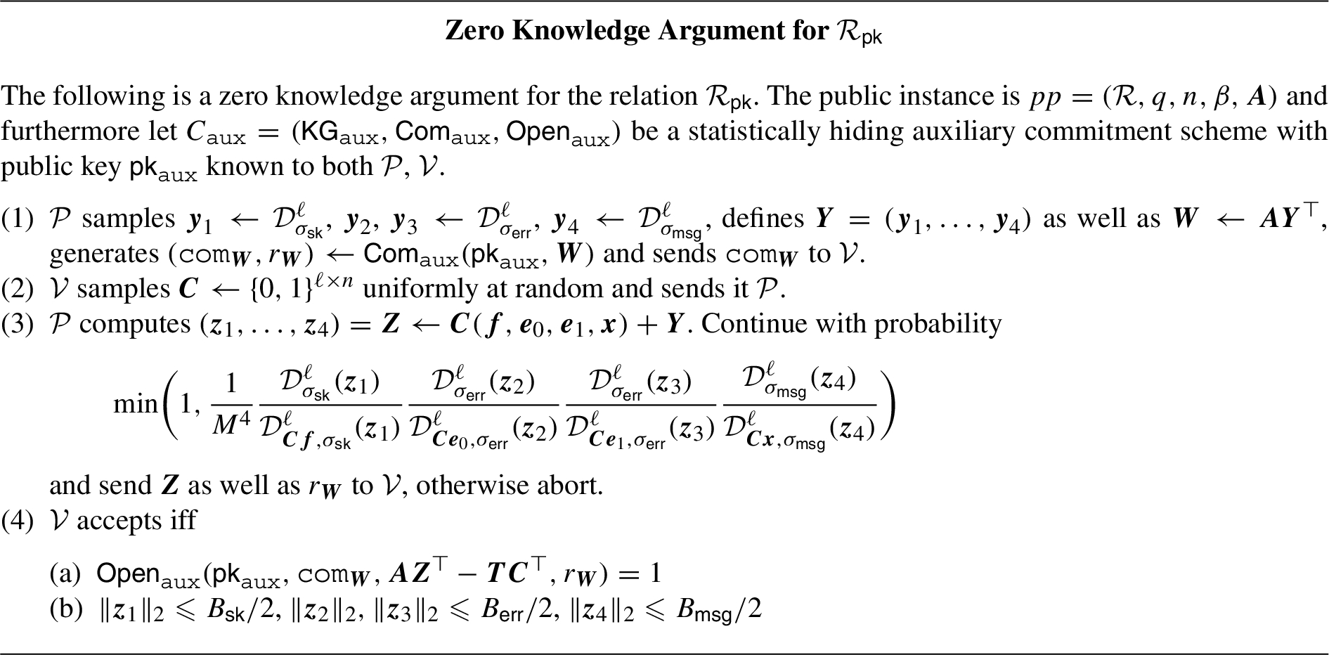
5.1. Argument for public OLE

Fig. 8.

Zero knowledge argument for $R_{pk}$ .

Recall the relations $R_{Alice}^{pk}$ and $R_{Bob}^{pk}$ considered in Section 3.2. We present in this section a zero-knowledge argument of knowledge for these relations. We begin by noticing that these relations can be expressed in matrix-form as $T = A S$ where $A$ is derived from the public parameters, $T$ is the target and $S$ is the secret we want to prove knowledge of. More concretely $\begin{matrix} \underset{A}{\underset{︸}{(\begin{matrix} b & 1 & 0 & 0 \\ - a & 0 & 1 & q / p \end{matrix})}} \cdot \underset{S}{\underset{︸}{{(\begin{matrix} f & e_{0} & e_{1} & x \end{matrix})}^{⊤}}} = \underset{T}{\underset{︸}{(c_{0}, c_{1})}} \end{matrix}$ where we show that $S$ has a bound of $B_{sk}$ , $B_{err}$ , $B_{err}$ , $B_{msg}$ for each row, respectively.

We consider one single relation $R_{pk}$ , defined as in $R_{Bob}^{pk}$ (or $R_{Alice}^{pk}$ ), but using the 2-norm instead of the ∞-norm.9

⁹

The choice of norm is irrelevant for the purpose of the existence of a proof, since bounds in one norm can be translated to the other.

To prove this relation, we use the interactive argument between

P

and

V

that is outlined in Fig. 8. We obtain the following theorem.

Theorem 6.

Assume that $\forall i \in [n] : ‖ f [i] ‖_{2} ⩽ T_{sk}$ , $‖ e_{0} [i] ‖_{2}, ‖ e_{1} [i] ‖_{2} ⩽ T_{err}$ , $‖ x [i] ‖_{2} ⩽ T_{msg}$ . Let $ℓ ⩾ κ + 2$ , $M > 1$ and $σ_{x} ⩾ 12 / (ln M) \sqrt{n ℓ} T_{x}$ . Furthermore, let $C_{aux}$ be a statistically hiding and computationally binding commitment scheme. Then the aforementioned protocol is a zero-knowledge argument of knowledge for $R_{pk}$ with $(B_{sk}, B_{err}, B_{msg}) = (\sqrt{8 N} σ_{sk}, \sqrt{8 N} σ_{err}, \sqrt{8 N} σ_{msg})$ that is complete with probability $1 / M^{4}$ , computationally sound and statistically zero-knowledge.

Proof.

The proof follows directly from Theorem 1 of [5] where the zero-knowledge argument is done individually for each row of $S$ using Lemma 3. We will therefore only sketch the most important parts.

Completeness. We will focus on the contribution of $f$ throughout the argument but it generalizes to $e_{0}$ , $e_{1}$ , $x$ accordingly. We know that for $i \in [n]$ it holds that $‖ f [i] ‖_{2} ⩽ T_{sk}$ . Thus $‖ (C f) [i] ‖_{2} ⩽ \sqrt{n} \cdot T_{sk}$ for all elements of the vector and hence $‖ C f ‖_{2} ⩽ \sqrt{ℓ n} T_{sk}$ . Using $σ_{sk}$ from the statement as well as Lemma 3 we can see that $Z$ will be sent with the required probability. As therefore particularly $z_{1} \sim D_{σ_{sk}}^{ℓ}$ we can upper-bound its norm using Lemma 2 setting $k = 2$ and using $N ≫ κ$ . Therefore Step 4b succeeds with overwhelming probability, while Step 4a holds by linearity.

Honest-Verifier Zero-Knowledge. In the simulation $S$ will simply sample $C$ as in the protocol, generate $\begin{matrix} (z_{1}, \dots, z_{4}) \leftarrow D_{σ_{sk}}^{ℓ} \times D_{σ_{err}}^{ℓ} \times D_{σ_{err}}^{ℓ} \times D_{σ_{msg}}^{ℓ}, \end{matrix}$ set $W \leftarrow A Z^{⊤} - T C^{⊤}$ and commit to the respective value $W$ . $S$ then outputs the transcript $(c_{W}, C, (r_{W}, Z))$ with probability $1 / M^{4}$ . Observe that indistinguishability follows by Lemma 3 as well as the statistical hiding property of $C_{aux}$ .

Soundness. By a standard heavy-column argument we can rewind a successful prover $P^{*}$ on different challenges for the same first message $c_{W}$ and are able to obtain multiple transcripts for different $(C, Z)$ , but fixed ${com}_{W}$ . Observe that by the binding property of $C_{aux}$ we must have that ${com}_{W}$ always opens to the same value. This allows us to obtain multiple equations of the form $T {(C - C^{'})}^{⊤} = A {(Z - Z^{'})}^{⊤}$ . We will extract $f [i]$ , $e_{0} [i]$ , $e_{1} [i]$ , $x [i]$ by rewinding with all columns of $C$ , $C^{'}$ being fixed during rewinding except for the i-th column, which means that all except for the i-th part of $T$ will disappear when being multiplied by ${(C - C^{'})}^{⊤}$ . Then by the aforementioned equation and the bounds on the $z_{i}$ from successfully produced transcripts the result follows. The lower bound of $ℓ ⩾ κ + 2$ is a consequence of the heavy-column argument of [5]. □

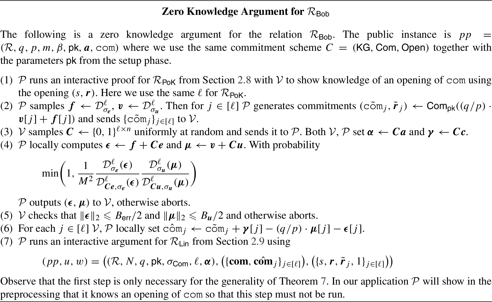
5.2. Argument for private OLE

For the OLE in Fig. 7 with preprocessing the relation which each party has to prove looks different from the aforementioned $R_{pk}$ and we cannot apply the same argument as above. In more detail, one of the two relations (the other follows along the same lines) that we want to prove is $\begin{matrix} R_{Bob}^{sk} = \{\begin{matrix} (p p, u, w) \\ = (\begin{matrix} (R, q, p, m, β, pk, a, com), \\ c, (u, e, s, r) \end{matrix}) \end{matrix} | \begin{matrix} (a, c, u, e) \in R_{q}^{n} \times R_{q}^{n} \times R^{n} \times R^{n} \\ \land c = (\frac{q}{p}) \cdot u + a \cdot s + e mod q \\ \land ‖ u ‖_{2} ⩽ B_{u} \land ‖ e ‖_{2} ⩽ B_{err} \\ \land {Open}_{pk} (com, s, r) = 1 \end{matrix}\} \end{matrix}$ where $β = (B_{u}, B_{err})$ .10

¹⁰
Observe that, again, we have switched to the 2-norm.

Towards constructing an interactive argument, we first observe that the equation to be proven can be alternatively written as $\begin{matrix} - a \cdot s = (q / p) \cdot u + e - c \end{matrix}$ which means that all such statements are in fact linear in s. At first glance it might seem plausible to apply a standard amortization technique such as in Fig. 8 but that is not possible: amortization techniques require that the instances are linear in a public value, whereas in our case we need to exploit linearity in the secret. In Fig. 9 we present a zero-knowledge argument for the specific relation whose overhead is $O (κ)$ , i.e. the number of additional vectors in $R_{q}^{n}$ only depends on the statistical security parameter κ.

Fig. 9.

Zero knowledge argument for $R_{Bob}$ .

Theorem 7.

Assume that $\forall i \in [n] : ‖ v [i] ‖_{2} ⩽ T_{u}$ , $‖ e [i] ‖_{2} ⩽ T_{e}$ . Let $ℓ ⩾ κ + 3$ , $M > 1$ and $σ_{x} ⩾ 12 / (ln M) \sqrt{n ℓ} T_{x}$ . Furthermore, let C be a statistically hiding and computationally binding commitment scheme. Then the aforementioned protocol is a zero-knowledge argument of knowledge for $R_{Bob}^{sk}$ with $(B_{u}, B_{err}) = (\sqrt{8 N} σ_{u}, \sqrt{8 N} σ_{e})$ that is complete with probability $1 / M^{4}$ , computationally sound and statistically zero-knowledge.

Proof.

The proof uses elements of the proof of Theorem 6, though some modifications are necessary to obtain the full statement.

Completeness. The proof of completeness follows along the exact same lines as the proof of Theorem 6, except that we now only have 2 vectors to perform rejection sampling on and not 4. All of the bounds can be determined the exact same way, and the correctness of the opening follows by homomorphism of the commitment scheme and the completeness of the arguments for $R_{PoK}$ and $R_{Lin}$ . We assume that both arguments succeed with probability $1 / M$ which yields the claim.

Honest-Verifier Zero-Knowledge. The simulator will start by a simulation of the argument for $R_{PoK}$ . If this sub-simulator outputs $τ_{1}$ then we will continue simulating, otherwise abort if the sub-simulator for $R_{PoK}$ aborts and output its aborting transcript.

As in the proof of Theorem 6, the simulator then generates $C \leftarrow {0, 1}^{ℓ \times n}$ honestly and samples $ϵ \leftarrow D_{σ_{e}}^{ℓ}$ , $μ \leftarrow D_{σ_{u}}^{ℓ}$ . Given this, we can compute $α$ , $γ$ as in the protocol.

Next, sample the commitments ${\hat{com}}_{j}$ as uniformly random commitments and generate the ${\tilde{com}}_{j}$ such that the equation from Step 6 holds. With probability $1 / M^{2}$ we output $(τ_{1}, {{\tilde{com}}_{j}}_{j \in [ℓ]}, C)$ and abort, otherwise we generate $τ_{2}$ as the output of the statistical zero-knowledge simulator of the argument for $R_{Lin}$ . Here, we abort and only output $(τ_{1}, {{\tilde{com}}_{j}}_{j \in [ℓ]}, C, ϵ, μ)$ if this sub-simulator aborts or otherwise output $(τ_{1}, {{\tilde{com}}_{j}}_{j \in [ℓ]}, C, ϵ, μ, τ_{2})$ if the sub-simulator succeeds.

Observe that the overall probability of outputting a full simulated transcript is $1 / M^{4}$ , a transcript without $τ_{2}$ $1 / M^{3}$ and a transcript only containing $τ_{1}$ with probability $1 / M$ which is the same as in the protocol. The values $ϵ$ , $μ$ are distributed as in the protocol by Lemma 3 whereas ${{\tilde{com}}_{j}}_{j \in [ℓ]}$ are statistically indistinguishable from those of the protocol due to the statistical hiding of the commitment scheme. Then, since $τ_{1}$ , $τ_{2}$ are statistically indistinguishable from the real transcript of the arguments for $R_{PoK}$ , $R_{Lin}$ the statement follows.

Soundness. Assume that there exists a prover $P^{*}$ that can convince a verifier with probability $ϵ > 2^{- κ + 3}$ . Observe that $P^{*}$ s randomness tape is fixed, except for the inputs coming from the interaction. We first rewind the prover on the subprotocol for $R_{PoK}$ where we extract the opening $(s, r, 1)$ . Observe that by the binding property of C $P^{*}$ is not able to open c to any $(s^{'}, r^{'}, f^{'})$ with $s^{'} \neq s$ throughout the rest of this argument.

Next, we fix some choice for $R_{PoK}$ and continue with the rest of the protocol with $P^{*}$ , calling this new hybrid algorithm $P_{1}$ . This fixes the commitments ${\tilde{com}}_{j}$ for the remaining protocol. By the standard heavy-column Lemma, with probability at least $1 / 2$ we have that the fraction of choices of $C$ and randomness in $R_{Lin}$ which make $P_{1}$ output a valid transcript is at least $2^{- κ + 2}$ .

Using the same fixing of $C$ we now arrive at a prover $P_{2}$ which with probability $1 / 4$ outputs valid transcripts with probability at least $> 2^{- κ + 1}$ . Using the soundness of $R_{Lin}$ in Step 7 we have that any ${\hat{com}}_{j}$ must contain a value of the form $- α [j] \cdot s$ for some $α [j]$ as $com$ in $R_{Lin}$ can only be opened to s due to the binding property of the scheme. Observe that these openings of ${\hat{com}}_{j}$ can be transformed into openings of ${\tilde{com}}_{j}$ by linearity of the scheme, i.e. they do also work for $P_{1}$ .

Next, using the same heavy-column argument as in the proof of Theorem 6 we can then for each $i \in [n]$ extract two accepting transcripts that have $C$ , $C^{'}$ where all columns of $C$ are identical to $C^{'}$ except for column i, which means that there is a j such that $\begin{matrix} - (α^{'} [j] - α [j]) s = γ [j] - γ^{'} [j] - (q / p) (μ [j] - μ^{'} [j]) - (ϵ [j] - ϵ^{'} [j]) \end{matrix}$ where by the definition of $α$ , $γ$ it must now hold that $\begin{matrix} a [i] \cdot s = c [i] - (q / p) (μ [j] - μ^{'} [j]) - (ϵ [j] - ϵ^{'} [j]) . \end{matrix}$ Setting $u [i] = μ [j] - μ^{'} [j]$ and $e [i] = ϵ [j] - ϵ^{'} [j]$ then yields the necessary values of the appropriate bounds. Observe that the loss in success probability is only constant (i.e. we can amplify it back by repeating the experiment) and that the extractor runs in expected time $poly (ϵ, κ)$ . □

In terms of complexity of the aforementioned protocol, we start by sending $ℓ = O (κ)$ commitments ${\tilde{com}}_{j}$ of $O (1)$ $R_{q}$ elements, then sample $ℓ \cdot n$ bits and then send two $R_{q}$ -vectors $ϵ$ , $μ$ which are of length ℓ each. Furthermore, we need to run a ZK argument of both relations $R_{PoK}$ , $R_{Lin}$ which each require additional $O (κ)$ $R_{q}$ -elements of communication (see Section 2.6. Therefore we obtain $O (κ)$ total communication.

5.3. On utilizing other zero-knowledge arguments

Both $R_{pk}$ and $R_{sk}$ can also be proven using other zero-knowledge arguments, and we will now explain why we chose this specific approach.

On individual arguments. An alternative to the use of amortized arguments such as those used in our protocol is to use arguments for each linear relation separately, e.g. using [10]. For n such instances the overall communication will then at least be $O (n N)$ and also computation must now be performed for each of the n instances. Amortization allows to instead reduce computation and communication to net κ instances, thus reducing the overhead.

On other amortized proofs. The recent work of [6] extended previous MPC preprocessing to use the more efficient challenge spaces of [5]. This can most likely be applied in our setting too and would lead to an earlier point at which amortization outperforms individual arguments. We leave this as interesting future work.

On generic proofs. Generic argument systems such as [2] or [13] outperform our proofs in terms of communication for large enough instances due to their sublinear (in the proven circuit) communication. This low communication comes at the expense of higher computation on the prover side, thus potentially decreasing the throughput of our protocol. [2,13] can use amortization over multiple instances, but so far it has not been studied how these perform in the lattice setting in comparison to specialized amortization techniques.

6. Evaluation

In this section, we evaluate the efficiency of our OLE protocols, and compare this with protocols based on previous techniques. Firstly, we look at the communication complexity and compare this with other protocols. Then, in Section 6.3, we present implementation results for our passively secure secret-key protocol to demonstrate its practicality.

6.1. Choosing parameters

We estimate parameters for our OLE protocols according to the correctness requirement in Proposition 2. For RLWE we use a ternary secret distribution (so, $B_{sk} = 1$ ) a Gaussian error distribution with $σ = 3.19$ and $B_{err} = 6 σ$ ; the soundness slack parameter is $τ = 1$ for passive protocols and $τ \approx 24 \sqrt{8 N n κ}$ otherwise. The statistical security parameter is $κ = 40$ .

6.2. Comparison to previous protocols

Table 1
Comparison of the complexity of our OLE protocols with previous works based on homomorphic encryption

Protocol Security Rounds * Total comm. (bits)

passive active $log m \approx 128$ $log m \approx 64$

passive active passive active

PK-OLE RLWE + FS † 1 1516 1630 1004 1120

SK-OLE RLWE + FS 1 758 815 502 560

AHE RLWE + FS + LOE ‡ 2 1320 1476 800 956

SHE RLWE + FS 2 3682 3682 2310 2310

RS noisy encodings – 8 4096 4096 2048 2048

Protocol	Security	Rounds *	Total comm. (bits)
PK-OLE	RLWE	+ FS †	1	1516	1630	1004	1120
SK-OLE	RLWE	+ FS	1	758	815	502	560
AHE	RLWE	+ FS + LOE ‡	2	1320	1476	800	956
SHE	RLWE	+ FS	2	3682	3682	2310	2310
RS	noisy encodings	–	8	4096	4096	2048	2048

1 round means that each party sends one message simultaneously. 2 rounds either means that each party sequentially sends one message (for AHE), or one simultaneous message, twice in succession (for SHE).

^†

FS is Fiat-Shamir.

^‡

LOE is linear-only encryption [15].

Table 1 presents the communication complexity, measured from the protocol specifications, of our two public-key and secret-key OLE protocols, and compares this with two other protocols based on RLWE-based homomorphic encryption, either additively homomorphic (AHE) or somewhat homomorphic (SHE), as well as a protocol based on noisy Reed–Solomon encodings (RS). As can be seen from the table, ours is the only protocol with just a single round of communication, where each party simultaneously sends just one message (as in a non-interactive key exchange), whereas both other protocols require two rounds. Our secret-key protocol, which requires some special preprocessing, has the lowest communication cost of all the protocols, with both passive and active security. Furthermore, compared with the previously most efficient protocol based on AHE with active security, our active protocols avoid the need for assuming linear-only encryption, which is a relatively strong and un-studied assumption, compared with standard RLWE.

A full description of these protocols can be found in Section 1.4.

6.3. Experimental results

We have implemented the passive version of the secret-key protocol (see in Fig. 7) in Go language, making use of the ring package provided by the lattigo library [41]. Our implementation features a full-RNS (Residue Number System) realization of all the protocol operations, using a moduli of 60-bit limbs. For comparison purposes, we have also implemented the AHE-based OLE protocol described in Appendix A. The implementation of the OLE passive protocol has been integrated into the lattigo library [41].

The execution times of the protocol steps were tested on a laptop with an Intel Core i7-8550U processor with 16 GB RAM, running Arch Linux with kernel 5.6.4 and Go 1.14.2 The latency is not simulated, as it is highly dependent on the particular deployment; we include instead the communication complexity of the involved messages, from which the latency can be derived.

Table 2

Parameter sets and run times in the passive case of Fig. 7

Parameter	Par. set 1	Par. set 2
q	360 bits (6 limbs)	480 bits (8 limbs)
p	240 bits (4 limbs)	360 bits (6 limbs)
m	60 bits (1 limb)	120 bits (2 limbs)
bit security	$\approx 159$	$\approx 116$
# OLEs	2097152	2097152

(a) Example parameter sets ( $n = 128$ and $N = 16384$ ) and global run times for the passive case of Fig. 7 (uniformly random ternary secret keys ${- 1, 0, 1}$ and Gaussian noise with $σ = 3.19$ ).

Bob	Par. set 1	Par. set 2	Alice	Par. set 1	Par. set 2
Step $2 . (a)$	$462 ms$	$601 ms$	Step $2 . (c)$	$564 ms$	$817 ms$
Step $2 . (d)$	$533 ms$	$772 ms$	Step $3 . (a)$	$350 ms$	$479 ms$
Step $3 . (c)$	$263 ms$	$438 ms$	Step $3 . (d)$	$242 ms$	$412 ms$
1st msg.	$995 ms$	$1373 ms$	1st msg.	$564 ms$	$817 ms$
2nd msg.	$263 ms$	$438 ms$	2nd msg.	$591 ms$	$890 ms$

(b) Run times in the passive case of Fig. 7 for the example parameter sets of Table 2(a) ( $n = 128$ and $N = 16384$ , uniformly random ternary secret keys ${- 1, 0, 1}$ and Gaussian noise with $σ = 3.19$ ).

Table 3

Total run times expressions and extrapolated run times in the passive case of Fig. 7

Run time expressions for Bob and Alice
$T_{Bob} = max (T_{2 . a} + T_{2 . d}, T_{3 . a} + T_{d}) + T_{3 . c}$
$T_{Alice} = max (T_{3 . a}, T_{2 . a} + T_{c}) + T_{2 . c} + T_{3 . d}$

(a) Total run time expressions for Bob ( $T_{Bob}$ ) and Alice ( $T_{Alice}$ ).

Total time	$600 Mbit / s$	$1 Gbit / s$	$10 Gbit / s$
Par. Set 1	$2526 ms$	$2023 ms$	$1344 ms$
Par. Set 2	$3508 ms$	$2837 ms$	$1931 ms$

(b) Extrapolated run times ( $max (T_{Bob}, T_{Alice})$ ) in the passive case of Fig. 7.

Table 4

Parameter sets and communication costs for the passive case of Fig. 7 and Appendix A

Parameter	Par. set 1	Par. set 2
${n, N}$	${256, 8192}$	${128, 16384}$
p	240 bits (4 limbs)	360 bits (6 limbs)
m	60 bits (1 limb)	120 bits (2 limbs)
bit security	$\approx 115$	$\approx 159$
# OLEs	2097152	2097152
Alice time	$1441 ms$	$2129 ms$
Bob time	$1024 ms$	$1375 ms$
Total time	$2465 ms$	$3504 ms$

(a) Example parameter sets and global run times for the passively secure OLE based on AHE from Appendix A (uniformly random ternary secret keys ${- 1, 0, 1}$ and Gaussian noise with $σ = 3.19$ ).

Proposed protocol of Fig. 7
{Bob \| Alice}	Par. set 1	Par. set 2
1st msg. {2.(a) \| –}	{94.37 \| –} MB	{125.83 \| –} MB
2nd msg. {– \| 3.(a)}	{– \| 62.91} MB	{– \| 94.37} MB
AHE-based protocol from Appendix A
1st round	{– \| 62.91} MB	{– \| 94.37} MB
2nd round	{125.83 \| –} MB	{188.74 \| –} MB

(b) Communication cost in the passive case of Fig. 7 and the passively secure OLE based on AHE from Appendix A.

We have chosen two practical parameter sets for both protocols (see Tables 2(a) and 4(a)), both featuring more than 110 bits of security,11

¹¹

We have used the LWE security estimator of Albrecht et al. [1] (available online in https://bitbucket.org/malb/lwe-estimator) to give bit-security estimates.

and achieving more than 2 million scalar OLEs per protocol run. Table 2(b) includes the run times corresponding to each party (Alice and Bob) and Table 4(b) (see Appendix A) shows the communication costs.

It is worth noting that the public key version from Fig. 5 is not explicitly tested, but it incurs in a similar computational complexity as the one from Fig. 7; it presents, though, an increase on the communication complexity, as the interchanged messages are composed of two polynomials instead of one.

As the latency is not simulated, in order to compare with other protocols, we must consider that the total run time of ours would be $max (T_{Bob}, T_{Alice})$ , being $T_{Bob}$ (resp. $T_{Alice}$ ) the corresponding run time for Bob (resp. Alice). Tables 3(a) and 3(b) include the corresponding expressions and also extrapolate total protocol run times for some specific values of network bandwidth ${600 Mbit / s, 1 Gbit / s, 10 Gbit / s}$ . $T_{step}$ corresponds to the time of each $step$ included in Table 2(b), and $T_{d}$ (resp. $T_{c}$ ) is the time needed to transmit ciphertext $d$ (resp. $c$ ).

Extrapolated runtimes are approximately equal or lower than those obtained with the protocol based on AHE from Appendix A; note that for the last one we are not taking into account transmission runtimes. Consequently, we can see that the proposed protocols in this paper achieve both a better efficiency and lower communication cost than the one based on AHE from Appendix A.

Footnotes

Acknowledgments

We thank the anonymous reviewers for comments which helped to improve the paper. This work has been supported by the European Research Council (ERC) under the European Union’s Horizon 2020 research and innovation programme under grant agreement No 669255 (MPCPRO), the Danish Independent Research Council under Grant-ID DFF–6108-00169 (FoCC), an Aarhus University Research Foundation starting grant, the Xunta de Galicia & ERDF under projects ED431G2019/08 and Grupo de Referencia ED431C2017/53, and by the grant #2017-201 (DPPH) of the Strategic Focal Area “Personalized Health and Related Technologies (PHRT)” of the ETH Domain.

Passively secure OLE from linearly homomorphic encryption

We start out with two parties having $u, v \in R_{m}^{n}$ as inputs where $P_{Alice}$ has $u$ and $P_{Bob}$ $v$ . Furthermore, assume that $P_{Bob}$ has $β \in R_{m}^{n}$ as well. Our goal is, again, to compute $α \in R_{m}^{n}$ such that $α + β = u ⋆ v$ . Here · is the product of ring elements or of a scalar multiplication with a vector, while ⋆ denotes the element-wise multiplication of two vectors.

First, $P_{Alice}$ samples $s \in R_{m}$ according to the ternary distribution, $c \in R_{p}$ uniformly at random as well as $r \in R^{n}$ as a discrete Gaussian with the same standard deviation $σ = 3.19$ (approximated using a Binomial distribution). It sends $p k = (c, d = c \cdot s + r)$ to $P_{Bob}$ .

In the first round of the OLE, $P_{Alice}$ samples $e_{1} \in R^{n}$ as a discrete Gaussian with the same standard deviation $σ = 3.19$ (approximated using a Binomial distribution). $P_{Alice}$ then samples $a \in R_{p}^{n}$ uniformly at random, computes $b = a \cdot s - (p / m) \cdot u + e_{1}$ and sends $a$ , $b$ to $P_{Bob}$ .

In the second round, $P_{Bob}$ samples $t \in R_{m}^{n}$ according to the ternary distribution, $e_{2} \in R^{n}$ according to a discrete Gaussian with $σ = 3.19$ but moreover $e_{3} \in R^{n}$ uniform with infinity norm smaller than $3 m N^{2} σ \cdot 2^{κ} < p / (2 m)$ . It sets $x = a ⋆ v + c \cdot t + e_{2}$ and $y = b ⋆ v + d \cdot t + (p / m) \cdot β + e_{3}$ and sends $x$ , $y$ to $P_{Alice}$ .

Finally, $P_{Alice}$ computes $α = ⌊ (x \cdot s - y mod p) / (p / m) ⌋$ and outputs this.

We see that

\begin{array}{l} x \cdot s - y & = (a ⋆ v + c \cdot t + e_{2}) \cdot s - b ⋆ v - d \cdot t - e_{3} - (p / m) \cdot β \\ = (a ⋆ v + c \cdot t) \cdot s + e_{2} \cdot s - (a \cdot s) ⋆ v - e_{1} ⋆ v - (c \cdot s) ⋆ t - r \cdot t \\ - e_{3} + (p / m) (u ⋆ v - β) \end{array}

and the desired relation holds. The noise terms add up to

r \cdot t + e_{1} ⋆ v + e_{2} \cdot s + e_{3}

where

e_{3}

due to its size statistically drowns the other three terms, which makes simulation possible. This is because

‖ e_{1} ‖_{\infty} ⩽ 6 σ

with overwhelming probability and

‖ v ‖_{\infty} ⩽ m / 2

, so

‖ e_{1} ⋆ v ‖_{\infty} ⩽ 3 m N^{2}

with overwhelming probability, while

r \cdot t

and

e_{2} \cdot s

are a lot smaller.

Furthermore, since we also require that $3 m N^{2} σ \cdot 2^{κ} < p / (2 m)$ this term will not lead to a wrap-around mod p during decryption and the result will be correct with overwhelming probability. Observe that $P_{Alice}$ will not actually have to send $a$ because it can be sampled from a PRG-seed by both $P_{Alice}$ , $P_{Bob}$ , meaning that the communication only requires 3 $R_{p}$ -elements for one $R_{m}$ -OLE once $p k$ is set up.

References

M.R.

Albrecht,

Player and

Scott, On the concrete hardness of learning with errors, J. Mathematical Cryptology9(3) (2015), 169–203, http://www.degruyter.com/view/j/jmc.2015.9.issue-3/jmc-2015-0016/jmc-2015-0016.xml . doi:10.1007/s10623-015-0048-8.

Ames,

Hazay,

Ishai and

Venkitasubramaniam, Ligero: Lightweight sublinear arguments without a trusted setup, in: ACM CCS 2017,

B.M.

Thuraisingham,

Evans,

Malkin and

Xu, eds, ACM Press, 2017, pp. 2087–2104. doi:10.1145/3133956.3134104.

Applebaum,

Cash,

Peikert and

Sahai, Fast cryptographic primitives and circular-secure encryption based on hard learning problems, in: CRYPTO 2009,

Halevi, ed., LNCS, Vol. 5677, Springer, Heidelberg, 2009, pp. 595–618. doi:10.1007/978-3-642-03356-8_35.

Applebaum,

Damgård,

Ishai,

Nielsen and

Zichron, Secure arithmetic computation with constant computational overhead, in: CRYPTO 2017, Part I,

Katz and

Shacham, eds, LNCS, Vol. 10401, Springer, Heidelberg, 2017, pp. 223–254. doi:10.1007/978-3-319-63688-7_8.

Baum,

Bootle,

Cerulli,

del Pino,

Groth and

Lyubashevsky, Sub-linear lattice-based zero-knowledge arguments for arithmetic circuits, in: CRYPTO 2018, Part II,

Shacham and

Boldyreva, eds, LNCS, Vol. 10992, Springer, Heidelberg, 2018, pp. 669–699. doi:10.1007/978-3-319-96881-0_23.

Baum,

Cozzo and

N.P.

Smart, Using TopGear in overdrive: A more efficient ZKPoK for SPDZ, in: SAC 2019,

K.G.

Paterson and

Stebila, eds, LNCS, Vol. 11959, Springer, Heidelberg, 2019, pp. 274–302. doi:10.1007/978-3-030-38471-5_12.

Baum,

Damgård,

K.G.

Larsen and

Nielsen, How to prove knowledge of small secrets, in: CRYPTO 2016, Part III,

Robshaw and

Katz, eds, LNCS, Vol. 9816, Springer, Heidelberg, 2016, pp. 478–498. doi:10.1007/978-3-662-53015-3_17.

Baum,

Damgård,

Lyubashevsky,

Oechsner and

Peikert, More efficient commitments from structured lattice assumptions, in: SCN 18,

Catalano and

De Prisco, eds, LNCS, Vol. 11035, Springer, Heidelberg, 2018, pp. 368–385. doi:10.1007/978-3-319-98113-0_20.

Baum,

Escudero,

Pedrouzo-Ulloa,

Scholl and

J.R.

Troncoso-Pastoriza, Efficient protocols for oblivious linear function evaluation from ring-LWE, in: Security and Cryptography for Networks – 12th International Conference, SCN 2020, Proceedings, Amalfi, Italy, September 14–16, 2020,

Galdi and

Kolesnikov, eds, Lecture Notes in Computer Science, Vol. 12238, Springer, 2020, pp. 130–149. doi:10.1007/978-3-030-57990-6_7.

10.

Baum and

Nof, Concretely-efficient zero-knowledge arguments for arithmetic circuits and their application to lattice-based cryptography, in: PKC 2020, Part I,

Kiayias,

Kohlweiss,

Wallden and

Zikas, eds, LNCS, Vol. 12110, Springer, Heidelberg, 2020, pp. 495–526. doi:10.1007/978-3-030-45374-9_17.

11.

Baum and

Nof, Concretely-efficient zero-knowledge arguments for arithmetic circuits and their application to lattice-based cryptography, in: Public-Key Cryptography – PKC 2020, Springer, 2020.

12.

Beaver, Efficient multiparty protocols using circuit randomization, in: CRYPTO’91,

Feigenbaum, ed., LNCS, Vol. 576, Springer, Heidelberg, 1992, pp. 420–432. doi:10.1007/3-540-46766-1_34.

13.

Ben-Sasson,

Chiesa,

Riabzev,

Spooner,

Virza and

N.P.

Ward, Aurora: Transparent succinct arguments for R1CS, in: EUROCRYPT 2019, Part I,

Ishai and

Rijmen, eds, LNCS, Vol. 11476, Springer, Heidelberg, 2019, pp. 103–128. doi:10.1007/978-3-030-17653-2_4.

14.

Bendlin,

Damgård,

Orlandi and

Zakarias, Semi-homomorphic encryption and multiparty computation, in: EUROCRYPT 2011,

K.G.

Paterson, ed., LNCS, Vol. 6632, Springer, Heidelberg, 2011, pp. 169–188. doi:10.1007/978-3-642-20465-4_11.

15.

Boneh,

Ishai,

Sahai and

D.J.

Wu, Lattice-based SNARGs and their application to more efficient obfuscation, in: EUROCRYPT 2017, Part III,

J.-S.

Coron and

J.B.

Nielsen, eds, LNCS, Vol. 10212, Springer, Heidelberg, 2017, pp. 247–277. doi:10.1007/978-3-319-56617-7_9.

16.

Boyle,

Couteau,

Gilboa and

Ishai, Compressing vector OLE, in: ACM CCS 2018,

Lie,

Mannan,

Backes and

Wang, eds, ACM Press, 2018, pp. 896–912. doi:10.1145/3243734.3243868.

17.

Boyle,

Couteau,

Gilboa,

Ishai,

Kohl,

Rindal and

Scholl, Efficient two-round OT extension and silent non-interactive secure computation, in: ACM CCS 2019,

Cavallaro,

Kinder,

Wang and

Katz, eds, ACM Press, 2019, pp. 291–308. doi:10.1145/3319535.3354255.

18.

Boyle,

Couteau,

Gilboa,

Ishai,

Kohl and

Scholl, Efficient pseudorandom correlation generators: Silent OT extension and more, in: CRYPTO 2019, Part III,

Boldyreva and

Micciancio, eds, LNCS, Vol. 11694, Springer, Heidelberg, 2019, pp. 489–518. doi:10.1007/978-3-030-26954-8_16.

19.

Boyle,

Gilboa and

Ishai, Breaking the circuit size barrier for secure computation under DDH, in: CRYPTO 2016, Part I,

Robshaw and

Katz, eds, LNCS, Vol. 9814, Springer, Heidelberg, 2016, pp. 509–539. doi:10.1007/978-3-662-53018-4_19.

20.

Boyle,

Kohl and

Scholl, Homomorphic secret sharing from lattices without FHE, in: EUROCRYPT 2019, Part II,

Ishai and

Rijmen, eds, LNCS, Vol. 11477, Springer, Heidelberg, 2019, pp. 3–33. doi:10.1007/978-3-030-17656-3_1.

21.

Brakerski,

Gentry and

Vaikuntanathan, (Leveled) fully homomorphic encryption without bootstrapping, in: ITCS 2012,

Goldwasser, ed., ACM, 2012, pp. 309–325. doi:10.1145/2090236.2090262.

22.

Brakerski and

Vaikuntanathan, Fully homomorphic encryption from ring-LWE and security for key dependent messages, in: CRYPTO 2011,

Rogaway, ed., LNCS, Vol. 6841, Springer, Heidelberg, 2011, pp. 505–524. doi:10.1007/978-3-642-22792-9_29.

23.

Chase,

Dodis,

Ishai,

Kraschewski,

Liu,

Ostrovsky and

Vaikuntanathan, Reusable non-interactive secure computation, in: CRYPTO 2019, Part III,

Boldyreva and

Micciancio, eds, LNCS, Vol. 11694, Springer, Heidelberg, 2019, pp. 462–488. doi:10.1007/978-3-030-26954-8_15.

24.

Cramer,

Damgård,

Xing and

Yuan, Amortized complexity of zero-knowledge proofs revisited: Achieving linear soundness slack, in: EUROCRYPT 2017, Part I,

J.-S.

Coron and

J.B.

Nielsen, eds, LNCS, Vol. 10210, Springer, Heidelberg, 2017, pp. 479–500. doi:10.1007/978-3-319-56620-7_17.

25.

Damgård,

Keller,

Larraia,

Pastro,

Scholl and

N.P.

Smart, Practical covertly secure MPC for dishonest majority – or: Breaking the SPDZ limits, in: ESORICS 2013,

Crampton,

Jajodia and

Mayes, eds, LNCS, Vol. 8134, Springer, Heidelberg, 2013, pp. 1–18. doi:10.1007/978-3-642-40203-6_1.

26.

Damgård,

Pastro,

N.P.

Smart and

Zakarias, Multiparty computation from somewhat homomorphic encryption, in: CRYPTO 2012,

Safavi-Naini and

Canetti, eds, LNCS, Vol. 7417, Springer, Heidelberg, 2012, pp. 643–662. doi:10.1007/978-3-642-32009-5_38.

27.

Damgård,

T.P.

Pedersen and

Pfitzmann, On the existence of statistically hiding bit commitment schemes and fail-stop signatures, in: CRYPTO’93,

D.R.

Stinson, ed., LNCS, Vol. 773, Springer, Heidelberg, 1994, pp. 250–265. doi:10.1007/3-540-48329-2_22.

28.

de Castro,

Juvekar and

Vaikuntanathan, Fast vector oblivious linear evaluation from ring learning with errors, 2020, https://eprint.iacr.org/2020/685.

29.

Dodis,

Halevi,

R.D.

Rothblum and

Wichs, Spooky encryption and its applications, in: CRYPTO 2016, Part III,

Robshaw and

Katz, eds, LNCS, Vol. 9816, Springer, Heidelberg, 2016, pp. 93–122. doi:10.1007/978-3-662-53015-3_4.

30.

Döttling,

Ghosh,

J.B.

Nielsen,

Nilges and

Trifiletti, TinyOLE: Efficient actively secure two-party computation from oblivious linear function evaluation, in: ACM CCS 2017,

B.M.

Thuraisingham,

Evans,

Malkin and

Xu, eds, ACM Press, 2017, pp. 2263–2276. doi:10.1145/3133956.3134024.

31.

M.F.

Esgin,

N.K.

Nguyen and

Seiler, Practical exact proofs from lattices: New techniques to exploit fully-splitting rings, in: ASIACRYPT 2020, Part II,

Moriai and

Wang, eds, LNCS, Vol. 12492, Springer, Heidelberg, 2020, pp. 259–288. doi:10.1007/978-3-030-64834-3_9.

32.

Genkin,

Ishai,

Prabhakaran,

Sahai and

Tromer, Circuits resilient to additive attacks with applications to secure computation, in: 46th ACM STOC,

D.B.

Shmoys, ed., ACM Press, 2014, pp. 495–504. doi:10.1145/2591796.2591861.

33.

Ghosh,

J.B.

Nielsen and

Nilges, Maliciously secure oblivious linear function evaluation with constant overhead, in: ASIACRYPT 2017, Part I,

Takagi and

Peyrin, eds, LNCS, Vol. 10624, Springer, Heidelberg, 2017, pp. 629–659. doi:10.1007/978-3-319-70694-8_22.

34.

Ghosh and

Nilges, An algebraic approach to maliciously secure private set intersection, in: EUROCRYPT 2019, Part III,

Ishai and

Rijmen, eds, LNCS, Vol. 11478, Springer, Heidelberg, 2019, pp. 154–185. doi:10.1007/978-3-030-17659-4_6.

35.

Gilboa, Two party RSA key generation, in: CRYPTO’99,

M.J.

Wiener, ed., LNCS, Vol. 1666, Springer, Heidelberg, 1999, pp. 116–129. doi:10.1007/3-540-48405-1_8.

36.

Ishai,

Kilian,

Nissim and

Petrank, Extending oblivious transfers efficiently, in: CRYPTO 2003,

Boneh, ed., LNCS, Vol. 2729, Springer, Heidelberg, 2003, pp. 145–161. doi:10.1007/978-3-540-45146-4_9.

37.

Ishai,

Prabhakaran and

Sahai, Secure arithmetic computation with no honest majority, in: TCC 2009,

Reingold, ed., LNCS, Vol. 5444, Springer, Heidelberg, 2009, pp. 294–314. doi:10.1007/978-3-642-00457-5_18.

38.

Keller,

Orsini and

Scholl, MASCOT: Faster malicious arithmetic secure computation with oblivious transfer, in: ACM CCS 2016,

E.R.

Weippl,

Katzenbeisser,

Kruegel,

A.C.

Myers and

Halevi, eds, ACM Press, 2016, pp. 830–842. doi:10.1145/2976749.2978357.

39.

Keller,

Pastro and

Rotaru, Overdrive: Making SPDZ great again, in: EUROCRYPT 2018, Part III,

J.B.

Nielsen and

Rijmen, eds, LNCS, Vol. 10822, Springer, Heidelberg, 2018, pp. 158–189. doi:10.1007/978-3-319-78372-7_6.

40.

Lyubashevsky, Lattice signatures without trapdoors, in: EUROCRYPT 2012,

Pointcheval and

Johansson, eds, LNCS, Vol. 7237, Springer, Heidelberg, 2012, pp. 738–755. doi:10.1007/978-3-642-29011-4_43.

41.

Lattigo 1.3.1, 2020, EPFL-LDS.

42.

Lyubashevsky,

Peikert and

Regev, A toolkit for ring-LWE cryptography, in: EUROCRYPT 2013,

Johansson and

P.Q.

Nguyen, eds, LNCS, Vol. 7881, Springer, Heidelberg, 2013, pp. 35–54. doi:10.1007/978-3-642-38348-9_3.

43.

Lyubashevsky and

Seiler, Short, invertible elements in partially splitting cyclotomic rings and applications to lattice-based zero-knowledge proofs, in: EUROCRYPT 2018, Part I,

J.B.

Nielsen and

Rijmen, eds, LNCS, Vol. 10820, Springer, Heidelberg, 2018, pp. 204–224. doi:10.1007/978-3-319-78381-9_8.

44.

Mohassel and

Zhang, SecureML: A system for scalable privacy-preserving machine learning, in: 2017 IEEE Symposium on Security and Privacy, IEEE Computer Society Press, 2017, pp. 19–38. doi:10.1109/SP.2017.12.

45.

Naor and

Pinkas, Oblivious transfer and polynomial evaluation, in: 31st ACM STOC, ACM Press, 1999, pp. 245–254. doi:10.1145/301250.301312.

46.

Rathee,

Schneider and

K.K.

Shukla, Improved multiplication triple generation over rings via RLWE-based AHE, in: CANS 2019, 2019, https://eprint.iacr.org/2019/577 .

47.

Regev, On lattices, learning with errors, random linear codes, and cryptography, in: 37th ACM STOC,

H.N.

Gabow and

Fagin, eds, ACM Press, 2005, pp. 84–93. doi:10.1145/1060590.1060603.

48.

Schoppmann,

Gascón,

Reichert and

Raykova, Distributed vector-OLE: Improved constructions and implementation, in: ACM CCS 2019,

Cavallaro,

Kinder,

Wang and

Katz, eds, ACM Press, 2019, pp. 1055–1072. doi:10.1145/3319535.3363228.

49.

N.P.

Smart and

Vercauteren, Fully homomorphic SIMD operations, Des. Codes Cryptography71(1) (2014), 57–81, ISSN 0925-1022. doi:10.1007/s10623-012-9720-4.

Proposed protocol of Fig. 7
{Bob \| Alice}	Par. set 1	Par. set 2
1st msg. {2.(a) \| –}	{94.37 \| –} MB	{125.83 \| –} MB
2nd msg. {– \| 3.(a)}	{– \| 62.91} MB	{– \| 94.37} MB
AHE-based protocol from Appendix A
1st round	{– \| 62.91} MB	{– \| 94.37} MB
2nd round	{125.83 \| –} MB	{188.74 \| –} MB

(b) Communication cost in the passive case of Fig. 7 and the passively secure OLE based on AHE from Appendix A.

Efficient protocols for oblivious linear function evaluation from ring-LWE 1

Abstract

Keywords

1. Introduction

1.1. Our contributions

1.2. Outline

1.3. Techniques

1.3.1. Efficient OLE from a public-key setup

1.3.2. Reducing communication with a dedicated setup

1.3.3. Achieving active security

1.4. Previous works

1.4.1. OLE from additively homomorphic encryption (AHE)

1.4.2. OLE from RLWE

1.4.3. OLE from somewhat homomorphic encryption (SHE)

2 This has slightly lower costs than the SPDZ protocol, since we have simplified the distributed decryption for the two-party OLE setting.

1.4.5. Other OLE protocols

2. Preliminaries

2.1. Rings & rounding

Definition 1 (Ring-LWE).

Definition 2 (Module-LWE).

Definition 3 (Module-SIS).

2.1.1. Rounding

Lemma 3 (Generalizes Theorem 4.6 of [40]).

Theorem 1 (See Theorem 4.6 of [40]).

3 Our protocols do not directly use the decryption algorithm, but our simulator in the proof of Theorem 3 does.

2.6. Commitments and zero-knowledge arguments

Commitment schemes

Zero-knowledge arguments of knowledge (ZKA)

4 The term “argument of knowledge”, in contrast to “proof of knowledge”, relates to the setting in which soundness is only guaranteed against a polynomially bounded prover.

Somewhat homomorphic commitments

2.8. Zero-knowledge proof of opening

8 As in public-key protocol from Section 3.2, P Alice does not need to prove the bound on her input v .

5. Zero-knowledge arguments

5.1. Argument for public OLE

10 Observe that, again, we have switched to the 2-norm.

6. Evaluation

6.1. Choosing parameters

6.2. Comparison to previous protocols

Footnotes

Acknowledgments

Passively secure OLE from linearly homomorphic encryption

References

²
This has slightly lower costs than the SPDZ protocol, since we have simplified the distributed decryption for the two-party OLE setting.

³
Our protocols do not directly use the decryption algorithm, but our simulator in the proof of Theorem 3 does.

⁴
The term “argument of knowledge”, in contrast to “proof of knowledge”, relates to the setting in which soundness is only guaranteed against a polynomially bounded prover.

⁸
As in public-key protocol from Section 3.2, $P_{Alice}$ does not need to prove the bound on her input $v$ .

¹⁰
Observe that, again, we have switched to the 2-norm.