
Abstract
Machine learning-based network intrusion detection systems have demonstrated state-of-the-art accuracy in flagging malicious traffic. However, machine learning has been shown to be vulnerable to adversarial examples, particularly in domains such as image recognition. In many threat models, the adversary exploits the unconstrained nature of images–the adversary is free to select some arbitrary amount of pixels to perturb. However, it is not clear how these attacks translate to domains such as network intrusion detection as they contain domain constraints, which limit which and how features can be modified by the adversary. In this paper, we explore whether the constrained nature of networks offers additional robustness against adversarial examples versus the unconstrained nature of images. We do this by creating two algorithms: (1) the
Introduction
Network intrusion detection systems (NIDS) have traditionally manifested as rule-based systems, such as Bro [42] and Snort [2]. However, with the rise in popularity of machine learning (ML), we are observing that machine-learning-based network intrusion detection systems are outperforming their rule-based counterparts [8,41,43,50]. While the performance of ML-based NIDS is compelling for widespread adoption and deployment, they are not void of their own limitations: when an adversary is introduced machine learning and the myriad of domains they serve often become vulnerable.
The field of adversarial machine learning (AML) explores the impact of adversarial examples: inputs to machine learning models that an attacker has designed to cause the model to make a mistake, e.g., misclassify [11]. Within the scope of this research, there have been studies that target particular inputs through a variety of threat models, with algorithms such as the
To date, many published works in adversarial machine learning have focused on unconstrained domains, that is, domains in which the adversary may arbitrarily select and perturb features by some parameterized cost (often measured through some
Furthermore, while there has been research that has focused on constrained adversaries[13,45], who are bound in their capabilities (for example, how many total features can be perturbed), we differentiate in that we consider constrained domains. Specifically, these constraints describe the kinds of inputs that are permissible in a domain (e.g., network packets that do not obey the TCP/IP protocol would not be permissible). In this work, we measure the efficacy of adversaries when subjected to the union of both adversary and domain constraints in networks, unlike previous work.
In this paper, we hypothesize that ML-based network intrusion detection systems are more robust to adversarial examples from two threat models: (1) from traditional adversarial algorithms, and (2) from universal adversarial perturbations. First, introduce the notion of primary features, which constrain the values other features can have. We design an algorithm to extract constraints from network datasets. Then, we develop an augmented algorithm, the We introduce domain constraints for network intrusion detection systems, and design an algorithm that is able to extract them systematically. Extracting constraints codifies the space of permissible adversarial examples. We introduce two algorithms: (1) The We perform experiments where we impose an extreme amount of adversary constraints, to the point where an adversary can only control five random features, and show that adversarial examples can still be crafted with a We demonstrate promising results for both algorithms, reaching greater than 95% misclassification rates across the datasets used in our experiments. This suggests that ML-based NIDS are comparably as vulnerable as their unconstrained counterparts, such as image recognition systems.
Background
Adversarial machine learning research for image recognition systems has been broad. Since the observations of Biggio et al. and Szegedy et al. in deep neural networks [3,46] to the robust attacks from Kurakin et al. and Sharif et al. [23,40], adversarial examples have matured from, “an intriguing property” to a tangible threat.
The first generation of attacks were formed in the context of “white-box” attacks [5,12,36]. Under this threat model, adversarial examples are crafted using information (e.g., model parameters) directly from the model under attack. This represents a worst-case scenario, analogous to an insider threat, since such information would not be easily accessible in most practical contexts. Naturally, this motivates the question: Can an adversary successfully attack a model, without having direct access to its parameters? Papernot et al. and Tramèr et al. investigated this question by leveraging transferability: an adversarial example crafted from one model will often be an adversarial example for a different model, even if they are using different training data and/or learning techniques [37,49]. Through this “black-box,” threat model, an adversary trains a surrogate model by using inputs to generate output labels from the victim model, called an oracle. Afterwards, the surrogate model is used to craft adversarial examples which are then (with high probability) “transferred” to the victim model.
Concurrently, others have investigated what limitations (if any) exist for adversarial examples. Kurakin et al. and Brown et al. explored how adversarial examples can be applied directly to the physical domain, introducing techniques that produce adversarial examples robust to physical distortions, such as rotation, scale, and other transformations [4,23]. Moreover, Goodfellow et al. and Moosavi-Dezfooli et al. analyzed universal adversarial perturbations: single perturbation vectors used to quickly craft adversarial examples from many inputs not known in advance [12,30]. These universal perturbations are especially concerning as they enable adversaries to take computation offline and amortize computational costs over many inputs compared to traditional, online attacks.
For this work, we modify an existing attack, the Jacobian-based Saliency Map Approach, introduced by Papernot et al. [36]. The
Most attack algorithms have upper limits on the allowable distortion they can introduce. This distortion is defined to be the distance between an adversarial example and its original counterpart. There are many metrics (principally
Unlike traditional image-based evaluations in adversarial machine learning, crafting adversarial examples for network intrusion detection systems is a necessarily different process. For one, the measurements used for bounding adversarial perturbations are simply inappropriate: traditional
Moreover, common assumptions in images allow adversaries to perturb features arbitrarily and independently – that is, any adversarial example is equally permissible in the domain. However, in networks, this assumption does not hold: a single network flow cannot connect to multiple services within the same packet, cannot set TCP flags on a UDP flow, cannot have negative round-trip times, among other constraints that, if ignored, adversarial crafting algorithms will produce. Thus, the threat model in networks is unique in that there are domain constraints that adversaries must obey for an adversarial example to be attack that represents a realizable traffic flow.
Finally, while there are some works that investigated the efficacy of adversaries in domains such as network intrusion detection, we find that the domain constraints: (1) are ignored [38,51], or (2) are explicitly avoided when applying perturbations [26]. Clearly, ignoring domain constraints in attack algorithms could produce adversarial examples that cannot be traced back to any traffic flow. Moreover, identifying features that are unconstrained reduces to the same approaches for attacking image data, in that adversaries are also free to perturb arbitrarily and independently, just with a smaller perturbation space. In this paper, we take an alternative stance where we produce adversarial examples while complying with the domain constraints.
Methodology
In this section, we explain the techniques used in adversarial machine learning (AML) for crafting adversarial examples, describe how we adapt them for network intrusion detection systems, and discuss our approaches used in the evaluation section.
AML for NIDS
Throughout, both in this section for examples and in the evaluation, we focus principally on network intrusion detection data (specifically, the use of TCP/IP). Network data is particularly compelling to use, as: (1) the underlying protocols encode complex constraints, (2) features are sourced from varying layers in the network stack (adding implicit constraints across layers), and (3) networks serve as a canonical domain for benchmarking practical uses of machine learning in security contexts. Here, we assume a network intrusion detection system classifies feature vectors (representing network traffic flows) as benign or malicious.2
Without loss of generality, the models we use in the evaluation discriminate between different kinds of network attacks (as well as benign traffic). Nonetheless, the goal of the adversary remains unchanged.
Crafting adversarial examples for NIDS is a necessarily different process from crafting adversarial examples against image recongition systems. Not all features represent the same kind of information (pixels vs packet information), nor do they describe the same kind of statistical data (discrete vs a blend of categorical, continuous, and discrete features). These differences change the threat surface and the underlying assumptions surrounding the capabilities of an adversary attacking a network intrusion detection system. Existing algorithms are unsuitable for attacking NIDS for these reasons:
Existing algorithms are largely optimized for human perception. While there is an open discussion on the amount and kinds of distortion that are appropriate [5], existing algorithms have been tuned for image domains [5,12,29]. That is, these algorithms try to minimize human perception of the distortion introduced in adversarial examples. However, such metrics have no meaning for many domains, including networks, because they are not perceived by humans. Thus, using algorithms optimized for human perception offers us limited utility, especially for network data. Existing algorithms assume adversaries have full control over the feature space. Most algorithms perturb the entire feature space to minimize an Existing algorithms do not consider domain constraints. Crafting adversarial examples that obey domain constraints is necessary to mount practical attacks. However, prior works strategically applied perturbations in order to explicitly avoid constraints [13,22] (such as only adding bytes at the end of a binary). While a reasonable strategy for malware, there are certainly applications of machine learning where constraint resolution cannot be trivially avoided. As an example of a constraint, network intrusion detection datasets commonly have protocol and service (port number) as features and certain services are exclusive to certain protocols. Therefore, to produce an adversarial example that is representative of a legitimate traffic flow, algorithms need to enforce these constraints.
Crafting with network constraints
In this subsection, we describe how we extract network constraints and incorporate them into crafting adversarial examples.
The concept behind primary features is harmonious with networks in particular. Many popular network intrusion detection datasets include features that represent services, flags, and other protocol-related information. Since these features share a causal relation with protocols, using transport layer protocols to be primary features is intuitive, as we then extract the relationships across many secondary features used in NIDS whose values directly depend on the protocol used (such as services and packet flags). Table 5 in the Appendix shows the constraints for one of the network datasets.
Given that constraints are restrictions on where and how features can be perturbed, it is intuitive to model these constraints as a simple form of first-order logic. Here, primary features are the predicates in logical expressions that determine the properties (e.g., values) that a collection of variables (e.g., secondary features) can have. Said alternatively, the set of primary features are the conditionals on the values of other secondary features. Formally, we can understand constraints to have the following form:
After primary features have been identified, we begin to extract constraints based on the following heuristic: a constraint exists between a primary feature k, and any other feature p, if there exists at least one input in the training set where both k and p are seen together. For example, features that describe TCP packet flags (i.e., p) would have the value 1.0 for TCP traffic flows (i.e., k) and 0.0 for non-TCP traffic flows. Therefore, TCP packet flag features are constrained to TCP flows. Conceptually, these constraints encode the maneuvers that are possible (and probable) for an adversary.
To allow the
This modification enables us to determine the optimal perturbation direction for increasing (the left half of the mask) or decreasing (the right half of the mask) features. Afterwards, we use the scoring metric found in [36] and return the most influential feature and optimal perturbation direction. Finally, the algorithm terminates when the input is misclassified or the
Consider the following example using the Algorithm 1. A UDP traffic flow is given to the

In this subsection, we describe how we create adversarial sketches:3
The concept of “sketching,” also known as approximate query processing [7], was first introduced by Flajolet et al. Sketching refers to a class of streaming algorithms that seek to extract information from a data stream in a single pass [10]. Commonly deployed in memory-constrained environments, these algorithms approximate or summarize the information in a given data stream. Adversarial sketches are similar as they are an approximation of a universal perturbation and computed through one pass of inputs.
For the same reasons described at the beginning of Section 3, existing algorithms to generate universal adversarial perturbations [4,16,30] are not immediately usable in networks: they are optimized for human perception, assume adversaries have full control over the feature space, and do not consider domain constraints.
In our search for adversarial sketches in networks, we take a principled approach using two tools: adversarial examples generated from the
With the universal perturbations discovered through the
While the
It is interesting to note that the
In this section, we evaluate our approach on two network intrusion datasets, the NSL-KDD and the UNSW-NB15, and two image recognition datasets, the GTSRB and MNIST. We answer two questions:
Do constraints add robustness against adversarial examples?
Do universal adversarial perturbations exist?
The experiments showed that we can craft adversarial examples with success rates greater than 95%, even with domain constraints; we can compute successful adversarial sketches, reaching greater than 80% misclassification rates for many learning techniques.
Our experiments were performed on a Dell Precision T7600 with an Intel Xeon E5-2630 and a NVIDIA GeForce TITAN X. We used CleverHans [34] for crafting adversarial examples.
Datasets
Before we describe our experiments, we provide an overview of the four evaluated datasets and any preprocessing that we performed. Table 1 describes the model architectures, hyperparameters, and model accuracies across all four datasets.
To measure the impact of network constraints on adversaries, we evaluate our approach on two network intrusion detection datasets and compare our results against two image classification datasets. While our image datasets do not contain constraints, we use them to: (1) compare the cross-domain generalization of our attacks (that is, the AJSMA and the HSG), and (2) provide a visualization of our techniques, which we detail in the Appendix.
Model information
Model information
The NSL-KDD contains 5 classes, with 4 attack classes and 1 benign class. It contains 125,973 samples for training and 22,543 samples for testing. It contains 41 features, separated into four high-level categories of features: basic features of TCP connections, content features within a connection suggested by domain knowledge, traffic features that are computed using a two-second time window, and host-based features. The NSL-KDD has been widely studied and so we defer to prior work [8,47] for the subtle details of the dataset. The state-of-the-art accuracy reported is 77.41% with Multi-layer Perceptrons [1,18,19,33,47].
The UNSW-NB15 contains 10 classes, with 9 attack classes and 1 benign class. It contains 175,341 samples for training and 83,332 samples for testing. The dataset contains 48 features, separated into four high-level categories of features: flow-based, basic connection, content, and time-based. We defer to the authors for a comprehensive description of the dataset [31] and its similarity with the NSL-KDD [32,33]. The state-of-the-art accuracy reported is 81.34% with an artificial neural network [28,32].
The MNIST database contains 10 classes, with numerical digits from 0 through 9. It contains 60,000 samples for training and 10,000 samples for testing. No preprocessing was required to integrate this dataset into our experimental setup. We defer to the authors for the intricate details surrounding the MNIST dataset [24]. The state-of-the-art accuracy reported is
The GTSRB contains 42 classes. After preprocessing, our experiments contained 21,792 samples for training and 6,893 samples for testing. Throughout the dataset, there are identical images of varying sizes. We first cropped the region of interest (which contains the traffic sign) and downsampled to a final size of
In this subsection, we describe our experiments in detail, using the NSL-KDD as an application of our approach.
Through our evaluation on network intrusion detection, we note that our experiments emulate a realistic adversary by taking different attacks and masking them as benign traffic.
For our inter-technique evaluation, we consider four popular learning techniques: Logistic Regression (LR), Decision Trees (DT), Support Vector Machine (SVM), and K-Nearest Neighbors (KNN). Each one of these learners represent different learning paradigms (and are popular in commercial and academic contexts), and are thus appropriate candidates for evaluating inter-technique transferability. Hyperparameters and other details can be found in the Appendix.
Next, we perform a stratified shuffle-split on the test set. This creates two sets of isolated inputs: we use the
Using the NSL-KDD as an example for the first stage, we built a Multi-layer Perceptron with 4 layers: an input layer of 123 units, fully-connected to 64 units, fully-connected to 32 units, and finally an output layer with 5 units.6
We note that the number of layers and units was influenced by research that suggests an optimal upper bound for the number hidden neurons for feed-forward networks [17]. The remainder of our hyperparameter selection follows no formal process.
NSL-KDD constraint distribution, categorized by feature type – Unlike TCP, UDP and ICMP have limited degrees of freedom
Output from crafting adversarial examples with the
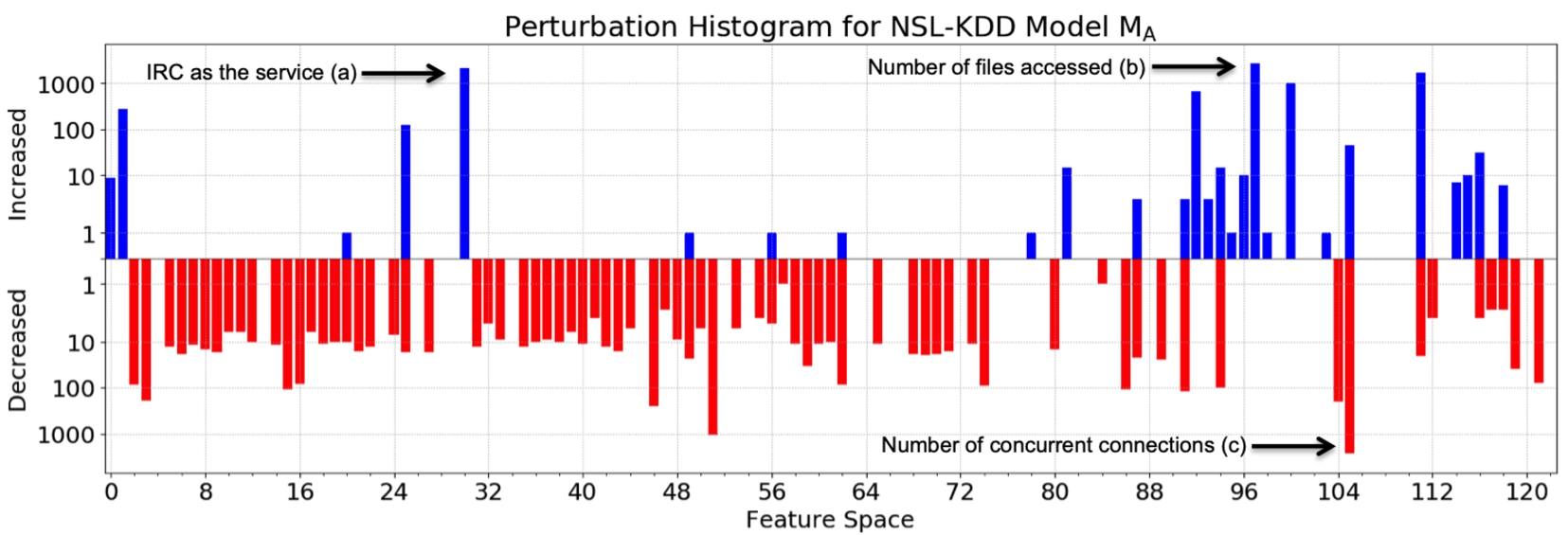
NSL-KDD model
We note that there are particular features that were consistently perturbed in nearly all adversarial examples, namely setting the service as
While it may seem this feature is not derived from network data, both the NSL-KDD and UNSW-NB15 have a “high-level content” category of features, which are derived from payload information.
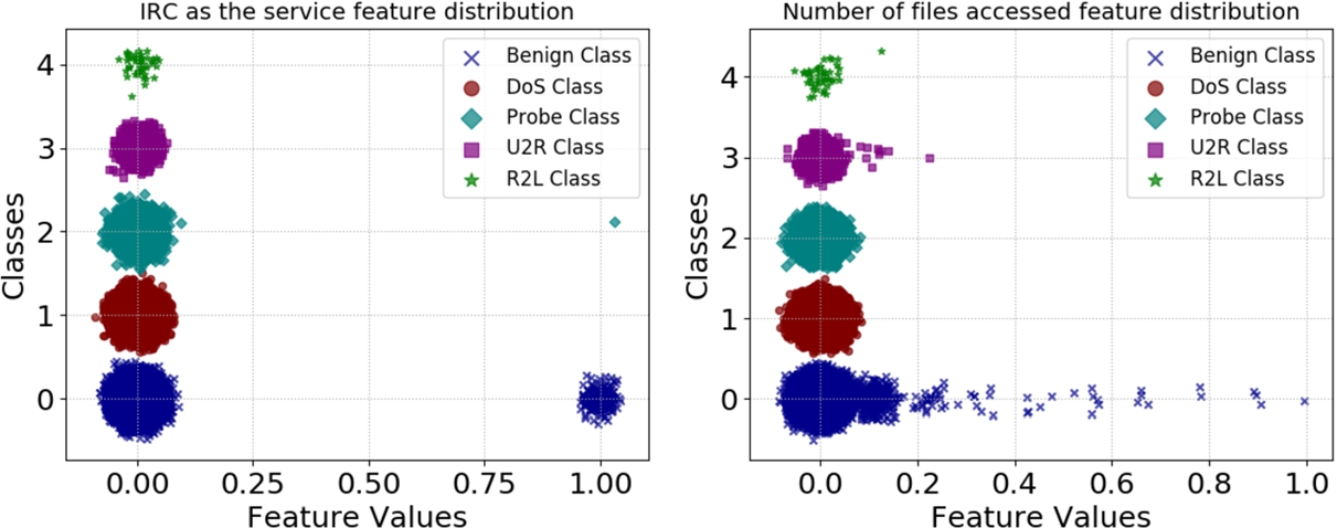
NSL-KDD class distribution for
With the adversarial examples crafted via the
We argue that measuring the accuracy of ML-based NIDS is appropriate for security validation, as accuracy gives network operators a metric by which to measure how the predictions of the NIDS conform to the expectation of network operators. Specifically, since ML-based NIDS rely on a labeled dataset from which to train, these labels are either (1) provided directly by network operators, or (2) provided through traffic analysis tools, such as IXIA Perfect Storm [31]. Thus, the efficacy of ML-based NIDS to produce predictions that conform to the provided labels aligns with expectations of security evaluations of such systems. Moreover, it also serves as the standard measurement in adversarial machine learning evaluations [5,11,30,36] and guides us to understand how adversaries would lay out attacks practically.
Specifically, an adversary would lay out an attack as follows: (1) the adversary would first use the
The choice of n is a function of the adversarial threat model; for our evaluation, we select an n for each dataset that roughly represents
Results for

Additionally, it is interesting that the adversarial examples produced by the
Finally, we are surprised at the fragility of the models trained on network intrusion detection data; sometimes perturbing only three features were necessary to misclassify greater than 80% of inputs in the test set. We believe that this fragility is partly a function of the skewed distribution certain features can have for specific classes, such as the ones shown in Fig. 2. This insight is unlike the adversarial examples crafted against image recognition systems, where high dimensionality and a more balanced class distribution for features appear to mitigate this fragility.
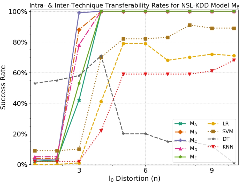
Table 4 shows the success rates for both of our algorithms across all four datasets. The values of n listed equal
We observe high success rates for both the
We hypothesize that this is partly due to how the
Moreover, we note that the inter-technique transferability rates were largely model-dependent. Specifically, we observe that relatively low transferability rates using the AJSMA, while the HSG maintains high transferability rates for the network datasets. This is likely due to the inherit design of the AJSMA – since the attack terminates immediately after an adversarial example is misclassified as benign traffic, we posit that adversarial examples are not sufficiently over the decision manifold for a source model that would also cross the decision manifold for other target models (since their decision manifolds would be slightly different). These results corroborate inter-technique transferability of adversarial examples produced by the JSMA in other experiments [37]. While we emphasize our evaluation principally on white-box attacks, we hypothesize that producing additional iterations of perturbations would raise the transferabiltiy rate, albeit at the likelihood of increased distortion, due to enforcing domain constraints.
From our investigation, we highlight some key takeaways:
Network constraints are not problematic for crafting adversarial examples in the datasets we studied. The
Universal adversarial perturbations that obey network constraints exist. The
Network intrusion detection data is highly fragile: a small dimensionality and biased distributions enable attack algorithms to alter very few features to successfully craft targeted adversarial examples that obey constraints.
Worst-case scenarios (i.e., white-box attacks) are highly vulnerable, not surprisingly. With access to model parameters, adversaries have sophisticated levels of control.
Network intrusion detection data appears to be highly vulnerable to transferability attacks. Even in the presence of disjoint training sets and different learning techniques, both attacks produced adversarial examples with surprising levels (an average of 73% for the
Throughout this paper, we have discussed some of the differences between adversarial machine learning in constrained networks versus unconstrained images. One of the most fundamental questions within this community is: what precisely is an “adversarial example?” There are varying definitions with different objectives used throughout AML research. In the image space, it has been generally agreed that if an attack algorithm produces perturbations that are undetectable by a human observer, then it is an adversarial example. However, it is not clear how this translates to other domains.
Research outside of image space (usually) provides their own definitions: perturbed malware must maintain its properties of malware [13,22], perturbed audio must be nearly inaudible [6], perturbed text must preserve its semantics [9,20], among other definitions. For our work in network intrusion detection, we follow an intuitive definition: perturbed network flows must maintain their attack behavior. For example, a denial-of-service attack must still deny service to an application or system, post-perturbation.
However, validating attack behaviors is a nontrivial task as security is contextual: DoS attacks on government networks have vastly different behaviors than attacks on small businesses. Therefore, any sort of simulation to observe attack behavior must be in a similar context to the one in which the dataset was built from. This is particularly challenging for old datasets like the NSL-KDD, as even a similar network setup would have different behavior given the modern hardware and software on the systems that would constitute that network. Even if all these factors could be accounted for, there are certain classes of attacks whose “success” is challenging to measure. For example, in reconnaissance attacks it is difficult to know if the information gathered by an adversary is useful.
Regardless, all of these points of contention are driven by a single hypothesis: Perhaps adversarial examples cannot be crafted if features which represent the semantics of the attack cannot be perturbed. Instead of attempting to justify why any set of features is critical to the semantics of the attack, we take a different stance on addressing this hypothesis: even if some reasonably sized subset of features could not be perturbed (as to not invalidate the attack semantics), we argue that adversarial examples can still be successfully crafted. With the lessons learned throughout our experiments, we set out to investigate this hypothesis with a straightforward experiment.
To test this hypothesis, we iterate over multiple sets of randomly selected features and make them unperturbable by the adversary. We repeat this random selection for sets of varying cardinalities from 1 to 41 features (where 41 represents the entire feature space). We train a new model on the full NSL-KDD training set and use the 100 most representative10
We find the most representative inputs by maximizing the difference (via the softmax layer) between the output component that corresponds to the label and the sum of the components that represent all non-label classes.
The “R2L” class only had 17 inputs that were correctly classified. Thus, we crafted from 317 inputs as opposed to 400.
The NSL-KDD has 41 features before expanding categorical features to one-hot vectors. If a particular combination contains a categorical feature, we eliminate all possible values associated with the feature from the search domain.
To prevent combinatoric explosion, we randomly sampled 1,500 unique combinations if the total number of possible combinations for a particular value of k exceeded 1,500. In total, we evaluated 55,723 unique combinations of unperturbable features.
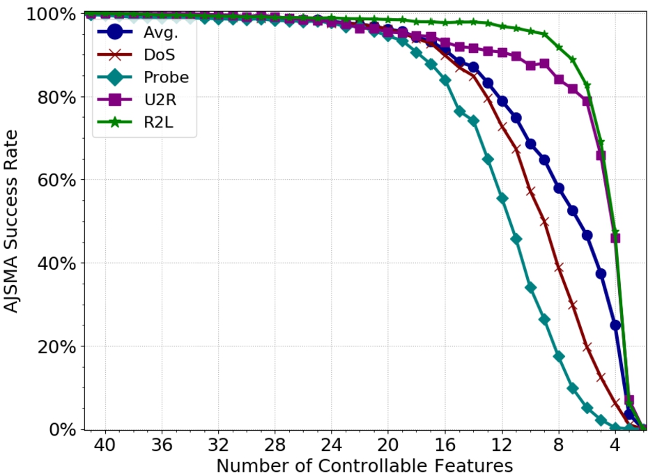
The results support our argument: the success rate of
Finally, we also highlight how this experiment demonstrates a type of constraint not covered in the evaluation section: features that the adversary simply does not have control over. Throughout this work, our constraints were defined via the semantics of the domain, i.e. the TCP/IP protocol. However, this experiment to preserve the semantics of the attack also serves as a demonstration of the efficacy of an adversary under this second type of constraints. These results suggest that even if an adversary maintains attack behavior and cannot arbitrarily control certain features and must obey the TCP/IP protocol, there is still a surprising amount of exploitable attack surface to craft adversarial examples.
In this section, we describe our thoughts for future work.
A more realistic adversary would be one would who want to execute a malicious payload over the network to another service – therein, the goal of the adversary is to simply have their traffic flow classed as benign, post-feature extraction. Manually curating a traffic flow such that, when extracted, conforms to the specification provided by adversarial examples is a non-trivial (and intractable) process. However, adversaries could leverage the very tools used to generate the attacks used in our evaluated datasets to an astonishingly precise degree. Specifically, the malicious traffic flows in the UNSW-NB15 (of whom features were extracted from), were generated by IXIA Perfect Storm traffic generator [31]. IXIA Perfect Storm can create malicious traffic flows subject to network profile constraints, attack constraints, service constraints, among others [14]. Thus, such traffic generators provide a means for adversaries to specify the constraints presented in an adversarial example, and map them back into real traffic flow.
In the absence of a machine-learning-based NIDS, adversarial examples can still be generated against rule-based systems, given knowledge about the underlying characteristics of the datasets used to form the rules. Specifically, for both the NSL-KDD and UNSW-NB15, Snort and Bro logs were used to create the feature vectors after the traffic flows were created. Thus, adversaries would then be equipped with knowledge of the information that would comprise the rules in a Snort or Bro NID system. However, since these rule-based systems are not differentiable (and thus, standard, gradient-based crafting technique would be inapplicable), adversaries would be required to manually construct feature vectors if the adversary knew the rules (as is done to attack non-differentiable learning algorithms, such as Decision Trees [37]), or query-based methods, commonly used in black-box attacks against machine learning classifiers [35].
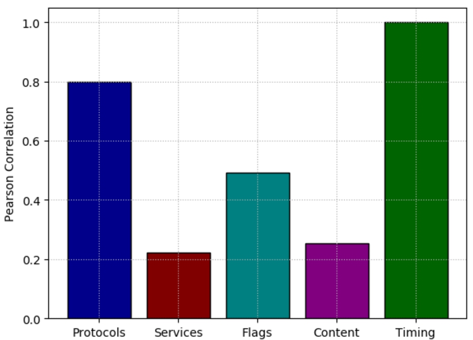
Normalized mean of summed absolute values of Pearson correlation coefficients for five categories of features in the NSL-KDD – Protocols are correlated with the majority of features, closely behind timing-based features, which are highly correlated amongst themselves.
In addition, we also observe that our approach for building adversarial sketches can also be used by a defender to assess model vulnerability. In particular, a defender could design a simple mechanism (driven by the perturbation histograms) that reveals universal directions that would make the model vulnerable. The defender can then use this analysis to detect adversarial examples at deployment. However, an adversary could circumvent detection by selectively perturbing features that have less impact. Naturally, this would come at a cost of introducing additional distortion and control over more features, which may be impractical for an adversary.
This paper investigated the impact of adversarial examples against ML-based network intrusion detection systems through the perspective of traditional adversarial algorithms and universal adversarial perturbations. In addition to this unique investigation into network intrusion detection, we introduced two new algorithms: the
Through our experiments, we observed how biased distributions coupled with low dimensionality can have an impact on model vulnerability, even with network constraints. Furthermore, we showed how when an adversary is constrained to five random features, adversarial examples can still be crafted with a
Prior to our work, the impact of adversarial learning has been understood in the context of unconstrained domains. We initially hypothesized that the constraints in networks would offer additional resilience to attack algorithms. However, our investigation suggests the inverse. Our two algorithms were able to craft adversarial examples with minimal distortion and with success rates of greater than 95% that also transferred to other models at rates up to 93%.
Footnotes
Appendix
Perturbation histogram for MNIST (a) and adversarial sketches for image datasets (b). The constraints extracted from the NSL-KDD – Unlike TCP, UDP and ICMP have limited degrees of freedom Scikit-learn model information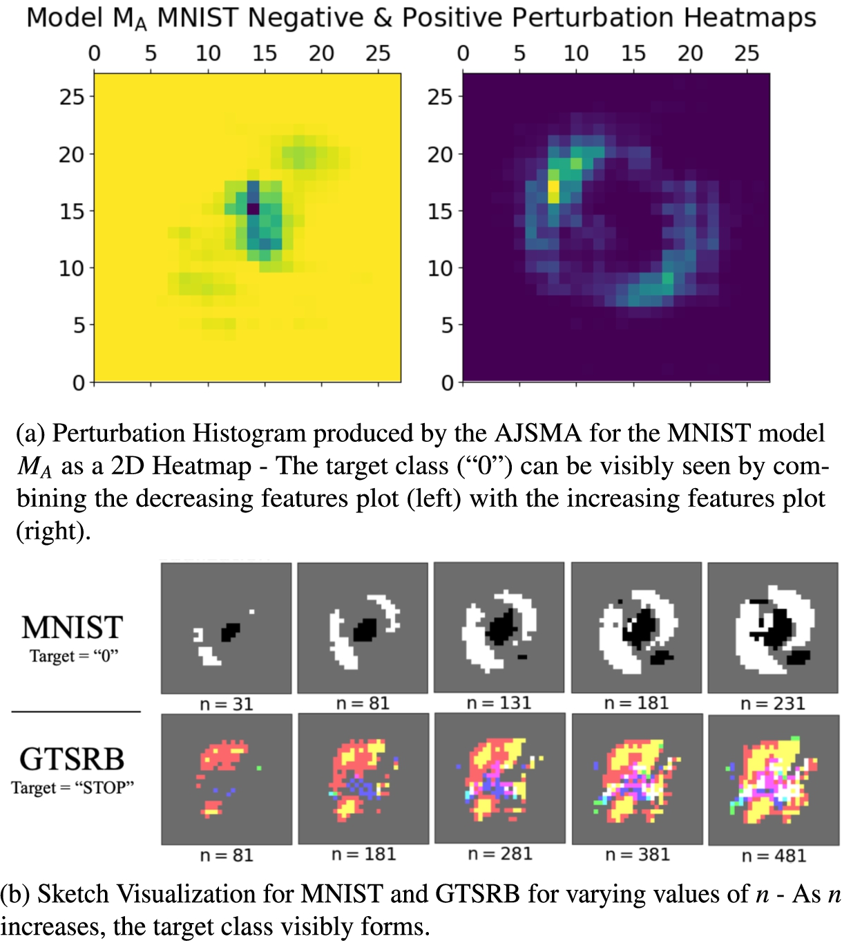
Protocol
Feature type
Basic
Content
Timing-based
Host-basted
duration, service=aol, service=auth, service=bgp, service=courier, service=csnet_ns, service=ctf, service=daytime, service=discard, service=domain, service=echo, service=efs, service=exec, service=finger, service=ftp, service=ftp_data, service=gopher, service=harvest, service=hostnames, service=http, service=http_2784, service=http_443, service=http_8001, service=IRC, service=iso_tsap, service=klogin, service=kshell, service=ldap, service=link, service=login, service=mtp, service=name, service=netbios_dgm, service=netbios_ns, service=netbios_ssn, service=netstat, service=nnsp, service=nntp, service=other, service=pm_dump, service=pop_2, service=pop_3, service=printer, service=private, service=remote_job, service=rje, service=shell, service=smtp, service=sql_net, service=ssh, service=sunrpc, service=supdup, service=systat, service=telnet, service=time, service=uucp, service=uucp_path, service=vmnet, service=whois, service=X11, service=Z39_50, service=34, flag=OTH, flag=REJ, flag=RSTO, flag=RSTOS0, flag=RSTR, flag=S0, flag=S1, flag=S2, flag=S3, flag=SF, flag=SH, src_bytes, dst_bytes, land=1, urgent
hot, num_failed_logins, logged_in=1, num_compromised, root_shell, su_attempted, num_root, num_file_creations, num_shells, num_access_files, is_host_login=1, is_guest_login=1
count, srv_count, serror_rate, srv_serror_rate, rerror_rate, srv_rerror_rate, same_srv_rate, diff_srv_rate, srv_diff_host_rate
dst_host_count, dst_host_srv_count, dst_host_same_srv_rate, dst_host_diff_srv_rate, dst_host_same_src_port_rate, dst_host_srv_diff_host_rate, dst_host_serror_rate, dst_host_srv_serror_rate, dst_host_rerror_rate, dst_host_srv_rerror_rate
duration, service=domain_u, service=ntp_u, service=other, service=private, service=tftp_u, flag=SF, wrong_fragment
count, srv_count, serror_rate, rerror_rate, same_srv_rate, diff_srv_rate, srv_diff_host_rate
dst_host_count, dst_host_srv_count, dst_host_same_srv_rate, dst_host_diff_srv_rate, dst_host_same_src_port_rate, dst_host_srv_diff_host_rate, dst_host_serror_rate, dst_host_rerror_rate
service=eco_i, service=ecr_i, service=red_i, service=tim_i, service=urh_i, service=urp_i, flag=SF, src_bytes, wrong_fragment
count, srv_count, serror_rate, rerror_rate, same_srv_rate, diff_srv_rate, srv_diff_host_rate
dst_host_count, dst_host_srv_count, dst_host_same_srv_rate, dst_host_diff_srv_rate, dst_host_same_src_port_rate, dst_host_srv_diff_host_rate, dst_host_serror_rate, dst_host_rerror_rate
Learning technique
Parameters
Test accuracy
Name
Value
NSL-KDD
UNSW-NB15
MNIST
GTSRB
l2
74.21%
67.65%
92.02%
84.94%
1.0
77.31%
69.02%
94.04%
84.3%
rbf
3
gini
74.52%
73.27%
87.73%
57.20%
∞
2
1
∞
5
74.90%
72.20%
96.88%
52.83%
2