Analysis of neural network detectors for network attacks

Abstract

While network attacks play a critical role in many advanced persistent threat (APT) campaigns, an arms race exists between the network defenders and the adversary: to make APT campaigns stealthy, the adversary is strongly motivated to evade the detection system. However, new studies have shown that neural network is likely a game-changer in the arms race: neural network could be applied to achieve accurate, signature-free, and low-false-alarm-rate detection. In this work, we investigate whether the adversary could fight back during the next phase of the arms race. In particular, noticing that none of the existing adversarial example generation methods could generate malicious packets (and sessions) that can simultaneously compromise the target machine and evade the neural network detection model, we propose a novel attack method to achieve this goal. We have designed and implemented the new attack. We have also used Address Resolution Protocol (ARP) Poisoning and Domain Name System (DNS) Cache Poisoning as the case study to demonstrate the effectiveness of the proposed attack.

Keywords

Network attack neural network adversarial example

1. Introduction

Network intrusion detection systems (NIDS), such as Snort [50] and Zeek [53], play an essential role in enterprise network security operations. With the rapid rise of deep learning technology, neural network(NN)-based detectors (e.g., [20,31,61,62]) have been deployed in the real world to complement the existing NIDS. For example, IBM [5] and Microsoft [24] have offered artificial intelligence-based security products. IBM QRadar [5] is an AI-powered solution that “consolidates log events and network flow data from thousands of devices, endpoints, and applications”. Microsoft Security Copilot [24] “surfaces prioritized threats in real time and anticipates a threat actor’s next move with continuous reasoning based on Microsoft’s global threat intelligence”. Acting as an “ally”, NN-based detectors enable accurate detection of attacks even those not seen earlier, before the corresponding intrusion detection rule is created. NN-based detectors are usually deployed in the real world as follows: the existing network traffic monitoring tools (e.g., routers, Wireshark packet sniffers) are reused to capture the captured packets, which are usually held in PCAP files, to a node where the NN-based detectors are running with machine learning libraries (e.g, PyTorch, TensorFlow).

Because adversarial examples [16,59] are recognized as potentially a very serious threat to systems that use machine learning models, NN-based NIDS have been triggering an increasing amount of interests in the research community. In particular, several works [17,49] have recently investigated the adversarial examples specific to NN-based NIDS, and they assume the following threat model: The data manipulation threat model. This threat model assumes that the adversary is able to directly manipulate (i.e. modify) the network data after it is captured (e.g., packets held in PCAP files) and/or processed (e.g., data samples), but before it is fed to the NN-based NIDS.

Although this threat model is coherent with the adversarial example studies [16,37] in other domains such as computer vision, it is very different from the threat model assumed by real-world NIDS [39]. When NIDS are deployed to defend against network attacks, the following threat model is assumed as a matter of fact: The de facto standard threat model. This threat model does NOT assume that the adversary is able to manipulate data after it is generated. Rather, this threat model assumes that the attacker can only take action before the data is collected. In another word, if the attacker wants to replay the adversarial example, he/she must modify network packets before they are sent out. Once the packets are sent and data are collected, the attacker can no longer intervene.

Regarding why the data manipulation threat model is not assumed by real-world NIDS, we have the following observations. First, most real-world network attacks only compromise non-admin user accounts, and such accounts have limited influence in network communications. For example, the attacker may have compromised a user account on one host, but he/she cannot directly manipulate the packets sent by another host which the compromised account has no access to. Second, packet capture repositories are usually guarded by strict access control and integrity protection. Countering such access control and integrity protection assumes additional capabilities of the attackers.

Based on the above observations, it is important to check whether the adversarial examples successfully generated under the data manipulation threat model are also successful under the de facto standard threat model. Specifically, the checking process consists of the following checkboxes: (a) whether the adversary can treat the generated adversarial examples as an adversarial attack packet; (b) whether the adversarial examples can be somehow converted to adversarial attack packets; (c) whether the target machine can be compromised by the back-converted packets; (d) whether the network communications with back-converted packets, after being collected and processed in the same way as what is required of the NN-based NIDS, is classified as benign.

Using the above attack procedure, we have checked 17 general-purpose adversarial-example generation methods. We will summarize the experiment results in Section 2. In short, we found that none of the adversarial examples generated in our experiments is still successful under the standard threat model.

In this work, we seek to develop a new approach which can generate successful adversarial examples under the de facto standard threat model. These successful adversarial examples are denoted as stealthy network attacks in this paper, since the proposed attack and the real-world network attacks follow the same threat model. Though there exist other works that present similar ideas [2,4], these works focus on aligning the feature space with the problem space. In another word, they try to generate adversarial examples in the feature space that satisfy constraints in the problem space. However, they adopt extensive feature engineering [4,17] or use network flow data [3,48,58], which makes it very difficult, if not impossible, to be verified with real network packets and replayed in real network attacks. To the best of our knowledge, this work is the first work addressing this challenge and actually test the effectiveness of adversarial attack packets in real attacks.

Our approach firstly uses masks to capture protocol constraints. Then, our approach adapts the existing adversarial example generation methods by applying masks to them. In particular, we make the following two main modifications: 1) we apply masks when generating perturbations; 2) when generating perturbed data samples, we confine and round all values to the valid range specified for each field. With these two modifications, our approach can generate constraint-satisfying adversarial examples. For multi-packet network attacks, our approach uses a record-and-replay mechanism to help address the session-level uncertainties that the adversary may face when performing stealthy attacks in a real network.

The main contributions of this work are as follows: 1) We developed the first approach which can generate successful adversarial examples under the de facto standard threat model. The adversary can use these adversarial examples to launch stealthy network attacks and evade NN-based NIDS. 2) We used ARP poisoning and DNS cache poisoning attacks as the case studies to demonstrate the effectiveness of the proposed approach.

The rest of the paper is organized as follows. Section 2 provides the background and highlights the motivation. Section 3 describes the NN-based detectors. Section 4 formally defines constraint-satisfying adversarial examples, and then presents our problem statement. Section 5 described our proposed approach. Section 6 presents the evaluation results of the proposed approach. Section 7 discusses several relevant issues. Section 8 summarizes the related work. Section 9 concludes the entire paper.

2. Background and motivation

2.1. Network attacks and NIDS

Network attacks are frequently used in Advanced Persistent Threats (APTs). Some common network attack types include probing, denial of service (DoS), Remote-to-local (R2L), etc. These attacks can often cause serious impacts. For example, ARP poisoning and DNS cache poisoning are two commonly seen network attacks belonging to R2L attack type. With ARP poisoning attack, attackers can intercept or redirect network traffics within the LAN to any desired MAC addresses. In DNS cache poisoning attack, a falsified DNS record with the fake domain-to-IP mapping will be added and persist in the local DNS server until it expires. Whenever a machine inquires the poisoned DNS server for the affected domain’s IP, it will get the fake IP address.

Signature-based, rule-based, and anomaly-based detection are commonly used to detect these network attacks. However, signature-based methods [19] can be easily fooled by slightly changing the attack payload; rule-based methods [50] need experts to formulate and regularly update rules; and anomaly based detection [22,40] tends to raise lots of false positives. Especially in attacks where attackers can intentionally craft their packets to make them seem legitimate, such as in ARP poisoning and DNS cache poisoning attacks, the aforementioned methods usually fall short. Therefore, new detection methods need to be explored.

2.2. ML-based network attack detectors

Recently, researchers have been applying traditional machine learning and deep learning techniques for network attack detection. Support vector machine (SVM) [26,27], K nearest neighbors (kNN) [42,47], and decision tree (DT) [23,30], etc. have all been applied on public cybersecurity datasets like KDD CUP 99 [52] and NSL-KDD [45]. Though many of these works present satisfying detection results, traditional “shallow” machine learning approaches share the common drawback of requiring extensive feature engineering. If data samples are represented with minimal feature engineering, traditional machine learning algorithms may not be able to achieve comparable performance with deep learning [62]. For compensation, dimension reduction (like principal component analysis) has been proposed, but this can cause loss of information.

In recent years, deep learning-based NIDS is attracting more attentions, where feature engineering is performed by the neural network internally. DeepDefense [60], applying recurrent neural networks (RNN) for DoS detection, achieves higher than 97% accuracy; PCCN [61] which uses convolutional neural networks (CNN) to detect abnormal network traffic flows, can achieve higher than 99% accuracy; Long-Short Term Memory (LSTM) neural network has also demonstrated an accuracy of higher than 99% for detecting network attacks [20]. Many industries, including Splunk [51], FireEye [55], and Fortinet [14], etc., are incorporating deep learning into their network security products. One recent work [62] also studies applying deep learning techniques to the detection of two network attacks: ARP poisoning and DNS cache poisoning. The best trained deep learning models are quite accurate: for ARP poisoning, the detection rate is about 99.8%; for DNS cache poisoning, the detection rate is 100%. In another word, evasion rates are about $1 - 99.8 % = 0.2 %$ for ARP poisoning, and 0% for DNS cache poisoning. Therefore, blindly launching network attacks in the same old fashion without any countermeasures to evade neural networks is very likely to be detected. This will directly motivate attackers to alter their ways of launching network attacks.

2.3. Adversarial examples for DNNs

Adversarial examples are specialized data examples created with the purpose of confusing a DNN, resulting in the misclassification of a given data example. In the domain of computer vision, these adversarial data examples are indistinguishable to the human eye, but cause the DNN to fail to classify the corresponding images. In the domain of network security, these adversarial data examples cause the DNN to fail to classify the corresponding network data. A variety of automatic adversarial example generation methods have been proposed in the literature, and 17 of these methods will be shortly summarized in the next section.

2.4. Why the adversarial examples generated by existing methods fail under the standard threat model

Our experiments. Though there are works discussing domain-constrained adversarial examples, we did not observe any work verifying the effectiveness of adversarial examples in launching real network attacks. Therefore, we decided to do a preliminary motivating experiment. We tested 17 general-purpose adversarial example generation methods against the DNN trained to detect ARP poisoning attacks. (When we did the experiments, the 17 methods were all the methods that we are aware of.) The detection model and the datasets are from a prior work [62]. In particular, we followed the attack procedure described in Section 1, that is, we firstly used the 17 methods to generate adversarial examples against the DNN; then, generated adversarial examples are transformed to attack packets; finally, we ran the attack scripts (under the standard threat model) to directly send the attack packets to the target machine. After the attack packets were sent out, we used Wireshark to monitor/capture these packets. Every byte in the packet is then converted to numbers, so that every packet is represented as a vector, which is also a data sample to be fed into the detection model for classification.

The results are summarized in Table 1. The third column shows that 9 out of the 17 methods generated one or more adversarial examples, and in total more than 500 adversarial examples were generated. Unfortunately, the last column shows that none of the adversarial examples successfully compromised the target machine.

Why the existing methods failed. One reason is that the network packets also need to follow certain network protocol constraints (e.g. requiring certain values in specific fields). Another reason is that the attacker may only have limited control over the target network, and he/she cannot modify packets sent out from other machines. The existence of these two issues means that the adversarial attack packets can result in modifications of only a portion of a data sample fed into the NN-based detector, and the modifications need to satisfy certain constraints. For example, we examined the adversarial attack packets back-converted from the adversarial examples generated by the adversarial example generation method proposed in [11]. We found that majority of these packets are not recognized as ARP packets, because the value of the type field in the data link layer has been perturbed and is not ARP (0x0806). Although a small portion of the back-converted packets are correctly recognized as ARP packets (type field has value 0x0806), the values of the hardware type (HTYPE) field, the protocol type (PTYPE) field, or the hardware length (HLEN) field have been changed. However, in order to satisfy the ARP protocol constraints, none of these values should be changed; otherwise, the corresponding packets may be abandoned by the recipient. This is an elementary mistake, and no sensible attacker would fall for this, but it clearly shows that launching stealthy network attacks to evade NN-based detection is more than simply adopting adversarial example generation methods.

Table 1
General purpose adversarial example generation methods fail when launching the ARP poisoning attack

Adv. Ex. Gen. methods Time (s) Number of generated adversarial examples Number of successful ARP poisoning attacks using generated adversarial examples

FGSM [16] 0.02 0 0

BIM [28] 1.99 0 0

DeepFool [33] 0.73 98 0

JSMA [37] 0.51 0 0

VAT [32] 44.40 0 0

Carlini [9] 79.02 1 0

Inv. [21] 0.01 100 0

NewtonFool [25] 20.25 0 0

ZOO [12] 144.92 100 0

Boundary [6] 280.77 0 0

EAD [11] 369.10 89 0

PGD [29] 0.33 1 0

BBA [7] 33.44 0 0

DDNA [46] 0.57 5 0

Gen [1] 688.50 98 0

SLIDE [56] 0.33 0 0

HSJA [10] 2273.94 96 0

Adv. Ex. Gen. methods	Time (s)	Number of generated adversarial examples
FGSM [16]	0.02	0
BIM [28]	1.99	0
DeepFool [33]	0.73	98
JSMA [37]	0.51	0
VAT [32]	44.40	0
Carlini [9]	79.02	1
Inv. [21]	0.01	100
NewtonFool [25]	20.25	0
ZOO [12]	144.92	100
Boundary [6]	280.77	0
EAD [11]	369.10	89
PGD [29]	0.33	1
BBA [7]	33.44	0
DDNA [46]	0.57	5
Gen [1]	688.50	98
SLIDE [56]	0.33	0
HSJA [10]	2273.94	96

3. Dataset and detection neural networks

Before presenting our attack scheme, we will first introduce the detection neural network and the dataset on which the models are trained. In this work, we focus on the logic-flaw-exploiting (LFE) network attacks [62], which exploit the logic (security) flaws of a few widely-deployed authentication protocols. Such attacks are very different from other attacks such as memory corruption for code reusing, command and control (C&C) over HTTP/HTTPS, and (distributed) denial of service with/without botnet, etc. Memory corruption is more about the server program rather than the network protocol; C&C over HTTP/HTTPS assume the HTTP/HTTPS protocol itself is running normally; and (distributed) denial of service is usually accomplished by exhausting the server’s resources instead of exploiting a logic flaw within a protocol.

Two representative LFE network attacks are address resolution protocol (ARP) poisoning attacks and domain name system (DNS) cache poisoning attacks. ARP poisoning works by spoofing ARP responses, with which the attacker can trick the victim into falsified mappings between IP addresses and MAC addresses, and thus intervening the network communication. DNS poisoning works by spoofing DNS responses, with which the attacker can trick the victim into falsified mappings between domain names and IP address, and thus redirecting the network communication. Both of these two attacks exploit the lack of response verification in the corresponding protocol. As a result, the victims cannot verify whether the packets come from a genuine host or attacker. Also, these two attacks are difficult to be detected with traditional detection methods (e.g. signatures, rules, anomaly detections, etc.) because spoofing is applied (i.e. attacker packets are intentionally crafted to be indistinguishable from normal packets).

Table 2
Dataset statistics

Attacks Set Size Benign to malicious ratio

ARP poisoning Training 9584 1.005:1

Test 2400 0.982:1

DNS cache poisoning Training 30928 1.003:1

Test 7732 0.988:1

Attacks	Set	Size	Benign to malicious ratio
ARP poisoning	Training	9584	1.005:1
Test	2400	0.982:1
DNS cache poisoning	Training	30928	1.003:1
Test	7732	0.988:1

The detection neural networks and datasets are from another work [62], in which self-generated network datasets are generated due to lack of public datasets on the two attacks. This dataset is generated by adapting protocol fuzzing techniques, which can potentially generate new kinds of data not seen in publicly available datasets. The collected data is randomly split into a training dataset and a test dataset by ratio 4:1. Dataset statistics are shown in Table 2. The benign to malicious data sample ratio is kept at about 1:1 intentionally. Though this is different from the real-world network traffic, where the majority is benign traffic, the datasets for neural network training is balanced to avoid bias. That is, if the provided training datasets majorly contain benign data samples, then the trained neural network tends to predict data samples as benign. Balancing the benign to malicious ratio can mitigate such bias in neural network training. The dataset size is not very large, but, because we train separate neural networks for different network attacks, and that the neural network and data samples are not that complicated (details of which are presented in prior work [62]), we believe that the dataset size is sufficient for neural network training.

For ARP poisoning detection, a multi-layer perceptron (MLP) neural network is used, as shown in Fig. 1. Every data sample represents one network packet. 42 bytes are selected from each ARP packet. Every byte is then treated as a number when constructing data samples. Hence, each data sample for ARP poisoning is a 1D vector containing 42 integers.

For DNS cache poisoning detection, a convolutional neural network (CNN) is used, as shown in Fig. 2. The CNN’s input is 3D matrices. Firstly, starting from a whole network log, we filter out the DNS packets and chop them by sessions, resulting in multiple variate-length DNS sessions. Secondly, variate-length DNS sessions are chopped into fixed-length slices by applying a sliding window of size 6. 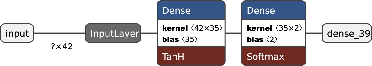Thirdly, in every DNS packet, 32 bytes from IP layer, UDP layer, and DNS layer are chosen. Each byte is converted to 8 bits, and then treated as an integer (0 or 1). As a result, every data sample for DNS cache poisoning is a 3D matrix of shape $6 * 32 * 8$ .

Fig. 1.

MLP neural network for ARP poisoning detection. Visualization by Netron1.

Fig. 2.

CNN for DNS cache poisoning detection. Visualization by Netron1.

When the models are used for detection, they take in different network packets. Specifically, ARP poisoning detection takes in ARP packets, and DNS cache poisoning detection takes in DNS packets. A packet sniffing process can be configured to sniff for ARP packets only, which will be processed and fed into the ARP poisoning detection model. The similar goes for DNS cache poisoning detection. The two models’ performances when detecting real attacks are summarized in Table 3. (Please refer to the original work for more details.) It can be inferred that, if the attacker takes no counter-measurements about the neural network detection, the attack is very likely to get detected.

Table 3

Test set evaluation results

Attack	ARP poisoning	DNS cache poisoning
Model architecture	MLP	CNN
Accuracy	99.75%	99.73%
F1 score	0.9975	0.9973
Detection rate	99.59%	99.53%
False positive rate	0.08%	0.08%

https://github.com/lutzroeder/netron

4. Problem formulation

4.1. Protocol-constraint-AWare adversarial examples

In this work, we first present a simple scenario, in which ARP poisoning is used as a running example for demonstration throughout the paper. The attack is completed with a single ARP packet, and the detection is also based on individual ARP packets.

As defined in Section 1, the attacker’s goal is to launch stealthy network attacks, which are accomplished by Protocol-Constraint-AWare (PCAW) adversarial examples. PCAW adversarial examples refer to the data samples that satisfy stealthy network attacks. PCAW adversarial examples have two intrinsic aspects: they are protocol-constraint-aware, meaning that they follow the protocol constraints; and they are adversarial examples, meaning that neural network detection models misclassify them. In ARP poisoning, they refer to data samples (generated from ARP packets) which can be used to launch the ARP poisoning attack, and are also misclassified by the detection model as benign.

A stealthy network attack contains at least two phases: 1) generating PCAW adversarial examples; 2) launching the stealthy network attack with the data from generated PCAW adversarial examples. The network packets that can lead to successful stealthy network attacks are called stealthy attack packets.

Constructing PCAW adversarial examples for attacks in phase 1 is much more challenging than constructing adversarial examples in computer vision: 1) Network communications must follow certain protocols; 2) The attack packets must have certain bytes so that these packets are valid and can exploit the vulnerability in the target machine/service.

Therefore, the following two challenges should be addressed:

How should the PCAW adversarial examples be generated for given neural network models?

How to launch stealthy network attacks with the help of generated PCAW adversarial examples?

For demonstration, we first use ARP poisoning attack [62]. The ARP poisoning attack is selected because: 1) The attacks can be detected largely, if not solely, based on network logs. Thus, neural network detection based on network logs is made possible. 2) The data samples of those detection neural networks present bytes from network packets, so the mapping between features in data samples and bytes in packets is straightforward. 3) There are no distinctive signatures for detecting these attacks. Thus, traditional detecting methods often fall short and deep learning can be applied. 4) The ARP poisoning attack represents single-packet network attacks, which is simpler than DNS cache poisoning, the multi-packet network attacks. It should be noted that, as long as the criteria 1 and 2 above are satisfied, our approach can also be applied to other network attacks, like Border Gateway Protocol (BGP) prefix hijacking.

4.2. Unique challenges in multi-packet stealthy network attacks

Extending the proposed stealthy attack packet generation method to the multi-packet network attack scenario has some unique challenges.

Assuming that one multi-packet attack session consists of eight packets $S = [x_{1}, x_{2}, x_{3}, x_{4}, x_{5}, x_{6}, x_{7}, x_{8}]$ , where packets $x_{3}$ and $x_{7}$ are attacker’s packets. A common data processing technique to deal with this kind of data is sliding window. Assuming that a sliding window of window size 6 and step size 1 is applied, the session above is processed into three data samples denoted as $s_{1} = [x_{1}, x_{2}, x_{3}, x_{4}, x_{5}, x_{6}]$ , $s_{2} = [x_{2}, x_{3}, x_{4}, x_{5}, x_{6}, x_{7}]$ , and $s_{3} = [x_{3}, x_{4}, x_{5}, x_{6}, x_{7}, x_{8}]$ . All these data samples are generated from the attack session and are therefore labeled as malicious. The session S will be detected as an attack session if any of the data samples are classified as malicious by the neural networks. Therefore, to evade detection, all data samples should be misclassified as benign. Hence, the ideal solution for attackers is to modify $x_{3} \to x_{3}^{'}$ and $x_{7} \to x_{7}^{'}$ , so that $s_{1}^{'} = [x_{1}, x_{2}, x_{3}^{'}, x_{4}, x_{5}, x_{6}]$ , $s_{2}^{'} = [x_{2}, x_{3}^{'}, x_{4}, x_{5}, x_{6}, x_{7}^{'}]$ , and $s_{3}^{'} = [x_{3}^{'}, x_{4}, x_{5}, x_{6}, x_{7}^{'}, x_{8}]$ can be misclassified as benign, and meanwhile $x_{3}^{'}$ and $x_{7}^{'}$ can still lead to successful attacks. Consequently, $S^{'} = [x_{1}, x_{2}, x_{3}^{'}, x_{4}, x_{5}, x_{6}, x_{7}^{'}, x_{8}]$ will not be detected as an attack session by the neural networks, although it is actually malicious. To align with our definition, we call such attack sessions, $S^{'}$ , as stealthy network attack sessions: they can compromise the network, similar to any other network attacks, and also remain stealthy by evading the detection of neural network models.

Without compromising other machines, attackers have no control over packets sent by other machines. In another word, attackers can only modify their own attack packets, which usually results in a small portion of the data sample(s). As a result, generating PCAW adversarial examples will be difficult for such data sample(s) because only a small portion can be perturbed. In the example above, $s_{1} = [x_{1}, x_{2}, x_{3}, x_{4}, x_{5}, x_{6}]$ has only one attack packet ( $x_{3}$ ), which means the attacker can only modify this $x_{3} \to x_{3}^{'}$ to make $s_{1}^{'} = [x_{1}, x_{2}, x_{3}^{'}, x_{4}, x_{5}, x_{6}]$ a PCAW adversarial example. Not surprisingly this may have a low chance of success.

Apart from the difficulty of generating PCAW adversarial examples, stealthy multi-packet attacks also have challenges that stem from the nature of sessions. In multi-packet attacks and detections, one session usually corresponds to one or more data samples. In a malicious session, an attacker’s packet may appear in one or more data samples from this session, depending on how the session is processed into data samples. For example, in the aforementioned example, the attacker’s packet $x_{3}$ in session S is involved in three different data samples $s_{1}$ , $s_{2}$ , and $s_{3}$ . This creates some uncertainties for launching stealthy network attacks:

When generating adversarial examples from different data samples (e.g. $s_{1}$ , $s_{2}$ ) that contain the same packet (e.g. $x_{3}$ ), information related to this packet might be modified in different ways. It is difficult to accommodate and reflect the different modifications in just one packet.

Some data samples, which belong to the same session, might fail to produce adversarial examples. For example, $s_{1}$ might generate an adversarial example, which can be converted reversely to network packets including packet $x_{3}^{'}$ , but $s_{2}$ might fail to generate adversarial examples, meaning no packet $x_{3}^{'}$ can make this data sample misclassified.

Even if an attack packet $x_{3}^{'}$ can make all the three data samples misclassified, this $x_{3}^{'}$ might only work within this session S. Whether it is effective in other sessions is uncertain.

All these uncertainties should be mitigated after PCAW adversarial examples are generated, but before attacks are launched in real world.

5. Proposed stealthy adversarial attacks

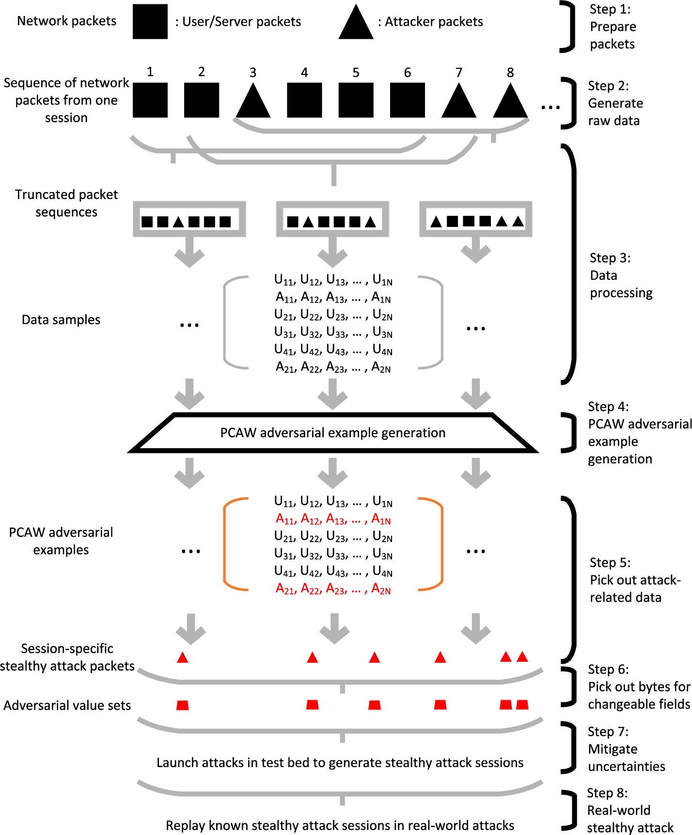
5.1. Work flow of stealthy network attacks

Fig. 3.

The work flow of launching stealthy network attacks.

The work flow (see Fig. 3) of the proposed stealthy network attacks is as follows:

Attackers prepare original packets.

In private test bed, attackers use the prepared attack packets to launch network attacks and gather network logs. Network logs contain packets from both normal users/servers and attackers, and are sorted in the time order.

Attackers process collected raw data into data samples.

Attackers feed data samples to the PCAW adversarial example generation tool to generate PCAW adversarial examples by only modifying changeable information in the attack packets.

From PCAW adversarial examples, attackers create candidate stealthy attack packets.

Attackers launch real-world network attacks by replaying known stealthy attack packets.

For the sake of simplification, we assume the white-box threat model, in which attackers can have full access to the target detection neural network. Attackers have different ways to accomplish this, like accessing the model with traditional cyber-attacks without compromising machines [54], or surrogate the target model [35,36].

5.2. PCAW adversarial example generation

One of the most important steps in the above flow is Step 4 – creating adversarial examples. To create adversarial examples from the original data samples, feature-based perturbations are usually used. Perturbation values are calculated based on the minimum component (feature) within the data sample, indicating the direction of how changes should be made to alter the model output. For example, if the perturbation for a feature is positive, increasing the value of this feature tends to change this data sample into an adversarial example. A problem that needs to be considered in this process is the existence of invariants, which are the packet features that should not be changed. 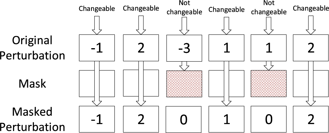To address this issue, we propose to use mask after the original perturbation is generated, as illustrated in Fig. 4. Mask is defined per minimum component of one data sample. For ARP poisoning, every data sample is a sequence of 42 integers, so the mask is also a sequence of 42 integers. The masks determine which values are changeable, and which are not. A byte/bit with mask value 1 means it is changeable, and 0 means it is unchangeable. By applying this mask, perturbations values corresponding to those unchangeable features will be reset to 0, which means no changes will be applied to these features. In this way, when the adversarial examples are converted back to network packets, the invariants are not changed and the resulting network packets are still valid.

Fig. 4.

Mask illustration.

To find out which fields in the packets are changeable, we refer to the protocol specifications to rule out fields related to the packet integrity, such as checksum and length fields. In addition, though some values (such as certain reserved bits) are marked as unchangeable in the protocol specifications, the servers may just ignore them in practice, so it is still safe to change them during perturbation. We launched network attacks in our test bed to find out such fields. For example, one changeable field is the time-to-live (TTL) in the IP layer. Though commonly set to 64, programs usually do not check the TTL value and simply let packets pass regardless. Therefore, this field is changeable for attackers: no matter how this value is changed, this packet will still be accepted rather than abandoned. As for fields related to the packet’s validity, such as checksum, they are decided after changes are made. In another word, we first generate the original attack packet, then change values in changeable fields, and finally re-calculate validity fields. Admittedly, after the checksum is re-calculated, the packet may not be adversarial. However, we do not run PCAW adversarial generation again because checksum is not controllable in real attacks. For example, the checksum field in the IP layer takes the identification field into calculation, and the value of the identification field changes very frequently. In our evaluations presented in Section 6.2, results also show that a secondary PCAW adversarial example generation is not necessary.

After we have generated the mask, we apply it in two well-known adversarial example generation methods, namely FGSM and ZOO.

Proposed Gradient-based Attack. FGSM is a well-known gradient-based evasion attack towards neural networks. FGSM takes the inputs of one original data sample as the seed, and the original model to extract gradients. The general workflow is as illustrated in Fig. 5a: 1) Given the original data sample and the target model, it calculates a perturbation specific to that provided seed with back propagation. 2) A perturbed data sample ( $X^{'}$ ) is generated by adding the original data sample (X) and the product of the perturbation (J) and a magnitude parameter λ, denoted as $X^{'} = X + λ * J$ . 3) In the end, $X^{'}$ is validated using the target model. If $X^{'}$ is misclassified, then this $X^{'}$ is an adversarial data sample; if not, then this attempt fails. To find more adversarial data samples, attackers may change the magnitude parameter λ or the original/seed data sample X, so that more different $X^{'}$ could be tried.

We modify the original FGSM for application in network attacks, as illustrated in Fig. 5b. Main changes include two parts: 1) masks are applied when generating perturbations; 2) during generating perturbed data samples, we confine and round all values to the valid range. Perturbations and the magnitude parameter may introduce decimal fraction or make values out of the valid range. For example, in ARP poisoning detection, every value should be integers within [0, 255]. In DNS cache poisoning, every value is either 0 or 1. Hence, these values should be confined and rounded.

Fig. 5.

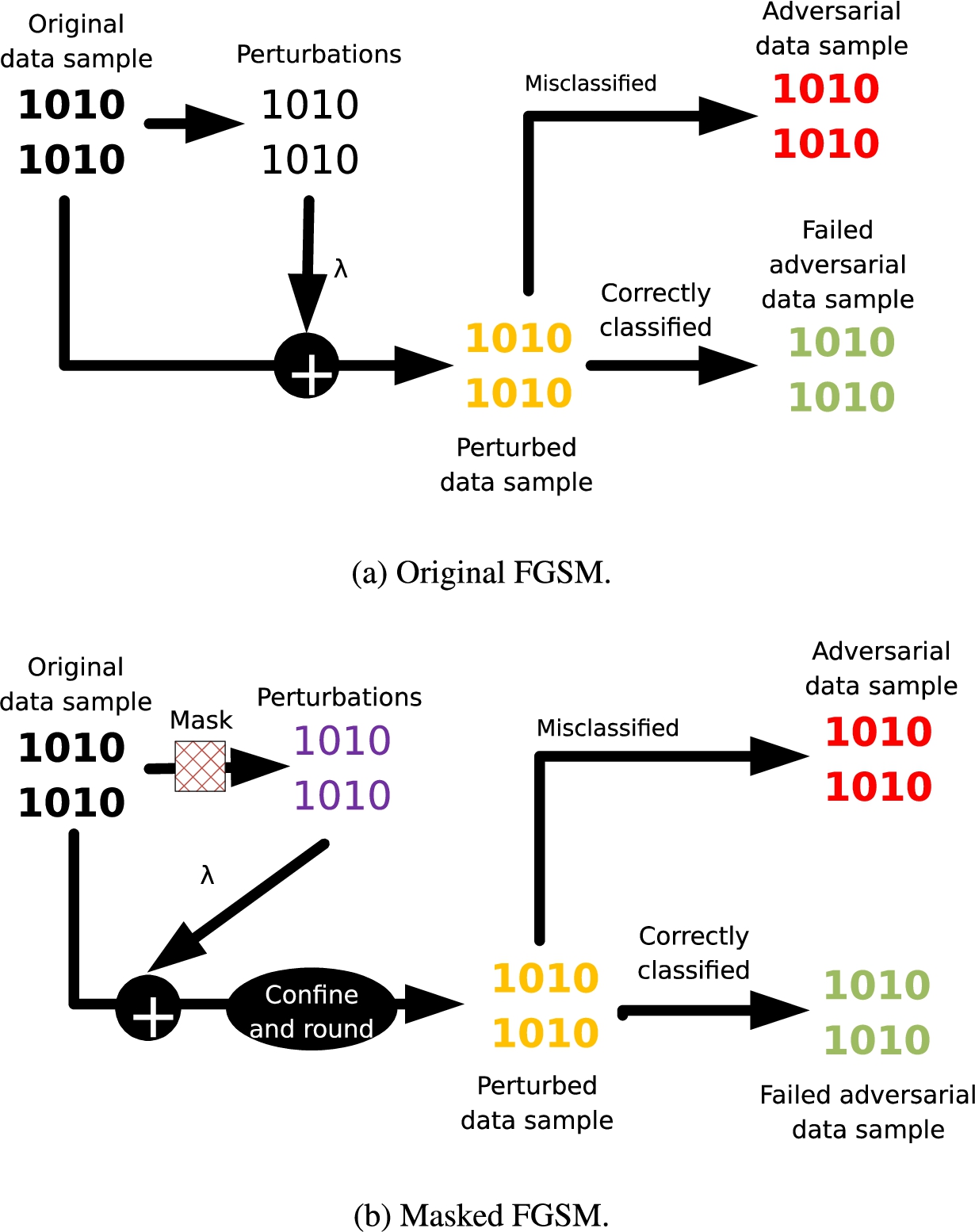
Illustration for FGSM.

Proposed Score-based Attack. For score-based attack, we propose a method based on the Zeroth Order Optimization (ZOO) [12]. Similar to FGSM, ZOO attack generates perturbations specific to the input data sample. Instead of calculating the gradient on the actual target model via back propagation, the proposed score-based attack estimates the approximate gradient using a finite difference method using the probability score which is output by the target model. The untargeted ZOO attack uses a hinge-like loss function $f (x)$ to measure the gap between the confidence score $F (x)$ of the original class label and the confidence scores of the other classes. It applies a small perturbation on original samples $x_{i 1} = x + h e_{i}$ and $x_{i 2} = x - h e_{i}$ , where $e_{i}$ is a standard basis vector and h is a small constant. Then it estimates the gradient $g_{i} = \frac{\partial f (x)}{\partial x_{i}}$ using symmetric difference quotient. With one more objective function evaluation, the Hessian estimate $h_{i}$ can be obtained. After estimating the gradient and Hessian for $x_{i}$ , we can use any first or second order method to approximately find the best perturbation δ to evade the NN model.

Algorithm 1:

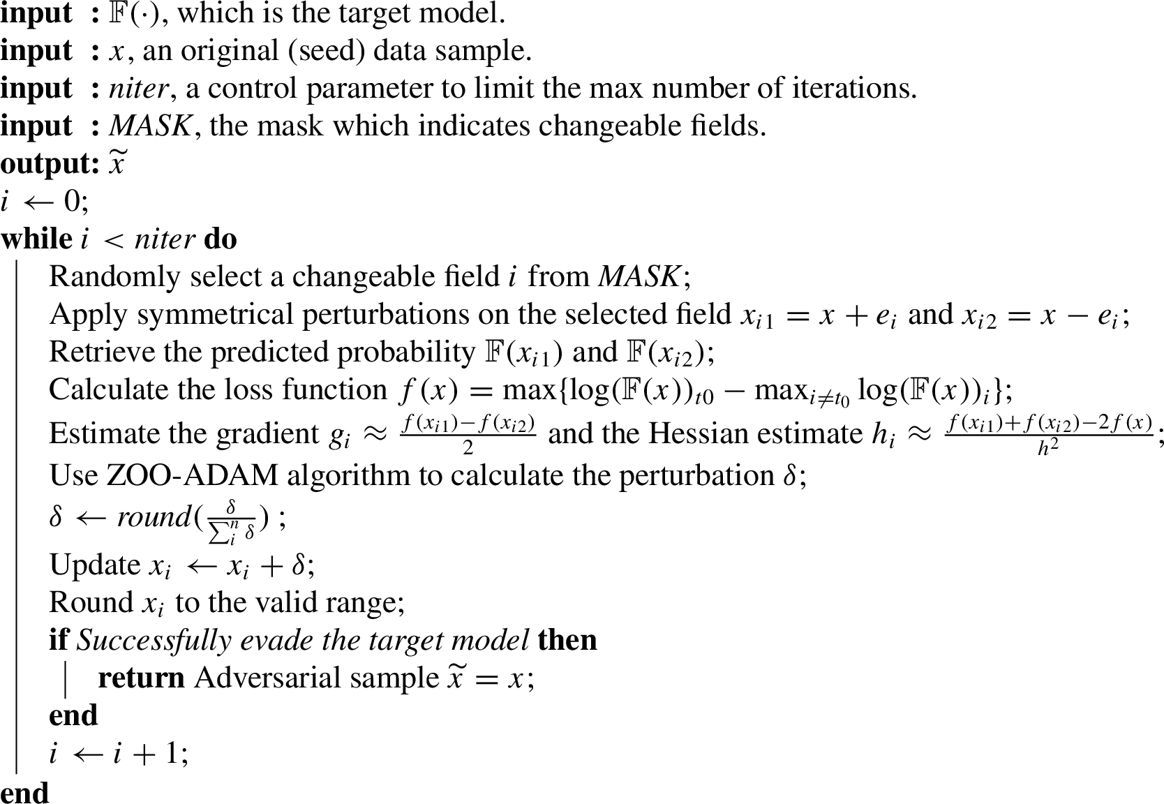
Proposed score-based attack

The proposed score-based attack is illustrated in Algorithm 1. First, changeable fields are randomly selected from the mask and a standard basis vector $e_{i}$ with only the i-th field as 1 is applied to obtain two symmetrical samples $x_{i 1}$ and $x_{i 2}$ . Then, those modified samples are fed to the target model $F (\cdot)$ to retrieve predicted probabilities $F (x_{i 1})$ and $F (x_{i 2})$ . Finally, Zeroth Order Stochastic Coordinate Descent with Coordinate-wise ADAM (ZOO-ADAM) is used to calculate the estimated gradient and the corresponding perturbation. The perturbation is not directly added to the original sample. The final perturbation is normalized and rounded to the valid range, which is $[0, 255]$ for ARP poisoning. Those steps repeat until the $niter$ iterations are completed, or the modified data sample successfully evades the target model.

5.3. Convert PCAW adversarial examples to candidate stealthy attack packets

As stated in Section 4, one of the reasons to choose ARP poisoning for demonstration is that, the conversion between data samples and network packets is straightforward. Basically, the back-conversion is a reverse process of data processing. In the case of ARP poisoning detection, each ARP packet is processed into one data sample with no information loss. Every byte in the original packet is preserved (except padding bytes) in the resulting data sample as a converted integer. Therefore, the back-conversion is to convert integers back to bytes in the original order to form a packet, and add padding bytes if needed. For more details, please refer to the data processing part in the work [62].

5.4. Mitigate uncertainties for multi-packet attacks

Fig. 6.

The threat model for stealthy multi-packet network attacks.

In Section 5.2, we ensure the packet’s validity by using mechanisms such as masks, value confine and round, but these mechanisms do not ensure the session’s validity. This subsection demonstrates how to use PCAW adversarial examples to launch stealthy multi-packet network attacks.

In Fig. 6, we present the threat model for stealthy multi-packet network attacks using DNS cache poisoning as an example:

Attackers prepare original attack packets.

In their own test bed, attackers use the prepared attack packets to launch network attacks, and gather network logs at the same time. Network logs contain packets from both normal users/servers and attackers, and are sorted in the time order.

Attackers truncate network logs into truncated packet sequences, which are in turn processed into data samples. Meanwhile, attack packets’ orders in data samples are recorded, to be used later.

Attackers feed data samples to the PCAW adversarial example generation tool to generate PCAW adversarial examples by only modifying changeable information in the attack packets, as the attack packets are the only ones that can be controlled by attackers.

From PCAW adversarial examples, attackers pick out the bytes related to attack packets (using the order information from before) if needed.

From session-specific attack packets, attackers select bytes for changeable fields to form adversarial value sets.

To mitigate the uncertainties discussed earlier, attackers use adversarial value sets to simulate the network attacks in his/her own test bed. Any successful stealthy attack sessions will be recorded in the adversarial value set database.

Attackers launch real-world network attacks by replaying known stealthy attack sessions from his/her simulations.

In a DNS cache poisoning attack, packet 1 corresponds to DNS query sent by the user, packet 2 corresponds to DNS query sent by the local DNS server, packet 3 corresponds to attacker’s spoofed DNS response, and packet 4 corresponds to global DNS server’s DNS response. Packets 5 and 6 correspond to the remaining steps or other DNS packets, and packets 7 and 8 stand for dummy attack packets, the impact of which will be discussed in Section 6.2. In the data samples, we use U to stand for bytes from user/server packets, and A to stand for bytes from attacker packets. The subscripts stand for position of bytes in the packets. For example, $A_{12}$ stands for the second selected byte from the first attacker packet.

For step 5 and step 6, we extract values of the changeable fields from generated PCA adversarial examples to create multiple “adversarial value sets”, each set corresponds to one original attack packet in one data sample. Step 6 and 7 are only needed for multi-packet attacks. Step 6 is necessary for DNS because the attack packets have to be crafted based on the user/server packets, and session-specific attack packets cannot be directly used in future attacks. That is why adversarial value sets are extracted: they are expected to carry the adversarial effects to evade neural networks. Step 7 is to mitigate the uncertainties by generating stealthy attack sessions in attackers’ own test bed. Those stealthy attack sessions can be used to build an adversarial value set database, to which attackers can refer in later real-world attacks. With this database, a patient and cautious attacker can persist in the LAN while sniffing packets. Only when a perfect attack chance appears will the attacker take action, trying to replay the stealthy attack session the attacker already knows. In this way, the three problems raised earlier are bypassed.

To generate stealthy attack sessions, the following factors can be used to reduce detection rates (DR) and possibly generate more stealthy attack sessions.

Dummy Attacker Packets. For DNS cache poisoning, since the detection is based on several continuous network packets, a natural choice of attackers is to send packets more diligently so that more attacker packets will be included in data samples, and therefore these samples will more likely be misclassified as benign. We call these packets sent by attackers as dummy attacker packets. To maximize the chances of blending dummy attacker packets into data samples, these dummy packets should be as similar to the real packets as possible, because attackers have no information about the way in which the defenders will filter and process network logs.

Attacker Packet Index. As discussed in Section 3, the data sample for DNS cache poisoning is a 3D matrix of shape $6 * 32 * 8$ , where 6 means that the data sample contains information of 6 network packets. Attacker packet index refers to how many attacker packets present in the data sample and where they are located inside the data sample. It is another factor that is out of attackers’ control. When network logs are processed into data samples, we divide them into different sessions and use a sliding window. All those processing is carried out at the defender’s side. Therefore, attackers have no idea where those attacker packets are located in the data samples. The number of attacker packets that get into the data samples can be indirectly affected by utilizing dummy attacker packets, but the index of attacker packets in data samples cannot be controlled by attackers in any way. As a result, attackers can only get the expected detection rates with respect to indices. Therefore, choosing a promising attacker packet index distribution is important for attackers.

After attackers have got stealthy attack sessions in their own test bed, they can build a database structured as in Fig. 7. The database consists of entry keys and sub-tables of key-value pairs. Each key is a hash value, each sub-table, marked by one specific entry key, represents a known stealthy attack session, and the values are the adversarial value sets. Each hash value is calculated based on the selected bytes from previous (up to 5, because the windows size is 6) packets in the session. Hash values are used as keys instead of directly comparing raw data for the sake of performance, because DNS cache poisoning attack requires quick response at the attackers’ side. If the entry key is matched, the corresponding stealthy attack session is selected to be replayed.

Fig. 7.

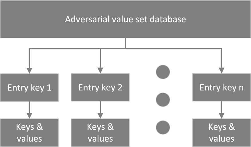
Adversarial value set database structure.

For example, in the DNS cache poisoning example, one session contains eight packets $S = [x_{1}, x_{2}, x_{3}, x_{4}, x_{5}, x_{6}, x_{7}, x_{8}]$ , of which x3 and x7 are attacker packets. Let’s assume that this session is a stealthy attack session. The entry key is calculated with $[x_{1}, x_{2}]$ , and the sub-table following this entry key has two rows: key $hash ([x_{1}, x_{2}])$ corresponding to $x_{3}$ , and key $hash ([x_{2}, x_{3}, x_{4}, x_{5}, x_{6}])$ corresponding to $x_{7}$ .

After the adversarial value set database is built, we use it to simulate a patient and cautious attacker. Such attacker will always wait for a perfect chance to take action. That is, this attacker will only send out attacker packets when the observed packets’ hash has a perfect match in the database. Even if the entry key is matched, as long as the observed packets at a later time does not match hashes in the sub-table, the attacker stops at once and let go of the current session. Taking the earlier example, the attacker will first wait for $[x_{1}, x_{2}]$ , and then send out $x_{3}$ . Only if this session is followed by $[x_{4}, x_{5}, x_{6}]$ , the attacker will send out $x_{7}$ , completing the replay of a known stealthy attack session. If not, the attacker stops at once and gets back to sniff for $[x_{1}, x_{2}]$ .

Adversarial Value Set Selection. Section 5.1 mentioned that the changeable fields of attacker packets will be replaced with a chosen adversarial value set to generate the stealthy attack packets. The selection of adversarial value set may affect the detection rate of neural networks. The attack packet is a direct response to the local DNS server’s query packet, so the selection of adversarial value set in the stealthy attack packet should be based on that query packet.

Therefore, we propose to build a dictionary that can be used to effectively search for the proper adversarial value sets. The dictionary consists of multiple entries; and each entry contains a key and one or more values. The keys in the dictionary are the DNS query packets sent out by the local DNS server. The values are the adversarial value sets. This dictionary can be created in the following way:

Map local DNS server’s query packet to the attack packet. This map is one-to-one.

Map the attack packet to the adversarial value set. This map is one-to-one or one-to-none, because not all data samples can be used to generate PCAW adversarial examples.

With the two steps above, establish the mapping between local DNS server’s query packet (as key) and the adversarial value set (as value).

Merge key-value pairs that have the same key.

When use the dictionary, we need to choose the adversarial value sets based on the keys. However, in actual attacks, we cannot guarantee that there is always an exactly matching key for the local DNS server’s query packet. Therefore, the distances between the query packet and the keys can be measured to find out the closest key. Depending on how the distance is defined, one observed local DNS query packet may refer to different entries. If the chosen entry holds multiple adversarial value sets (because of merging key-value pairs), one of them is randomly chosen. Assuming $x_{i}$ represents a byte in the local DNS server’s query packet, and $x_{i}^{'}$ represents a byte at the same position in the key, there are four commonly used distance measuring methods:

$L_{0} = count (x_{i} \neq x_{i}^{'})$ .

$L_{1} = \sum_{i}^{} | x_{i} - x_{i}^{'} |$ .

$L_{2} = \sqrt{\sum_{i}^{} {(x_{i} - x_{i}^{'})}^{2}}$ .

$L_{inf} = max (| x_{i} - x_{i}^{'} |)$ .

With the distance measuring method, the closest key is selected for each observed local DNS server query packet, and the corresponding entry is also determined. Please note that such distance measuring introduces additional processing time at the attacker’s side. However, for DNS cache poisoning to succeed, attacker’s packet has to arrive earlier than the global DNS server’s packet. To rule out the impact of the additional distance measuring time on the attack success, in our experiments, we manually insert time lags between the local DNS server and the global DNS server’s communications, so that attack packets always arrive earlier.

6. Evaluations

In this section, we will evaluate the effectiveness and efficiency of our proposed methods. Specifically, we want to answer the following evaluation questions:

Q1: How effective are our proposed stealthy network attack against ARP poisoning detection?

Q2: How effective are our proposed stealthy network attack against DNS cache poisoning detection?

Q3: How costly are our proposed methods?

All experiments are performed using a Windows machine equipped with an Intel Core i9-9900KS CPU and Nvidia RTX 3090 for accelerating computations. For software, we use Python 3.8.5, TensorFlow 2.4.1 with GPU support, ART 1.6.1 [34], and FoolBox 3.3.1 [43,44]. All data samples and trained detection models are retrieved from another work [62].

6.1. Q1: Stealthy ARP poisoning

Phase 1: PCAW adversarial example generation. We studied the performance of different PCAW adversarial example generation methods for ARP poisoning attack, including masked FGSM and masked ZOO. Table 4 shows results. We also added a category of “masked random” as the baseline, in which we only randomly changes the changeable portions regardless of gradients. For each method tried, we randomly select 100 data samples as the seeds to feed into PCAW adversarial example generation. The results show that masked FGSM is not effective, but is very fast; on the contrary, masked ZOO is slow, but generates more PCAW adversarial examples. The reason that masked FGSM fails to generate any PCAWAE is because we implement them differently. Masked FGSM changes multiple features in the data samples at a time, but masked ZOO changes one feature at a time. Therefore, masked ZOO works on a smaller granularity and can potentially find more PCAWAE. As a result, in Table 4, though masked ZOO finds 36 PCAWAEs, masked FGSM finds none.

Table 4
Proposed PCAW adversarial example generation methods’ performances towards ARP poisoning detection

Proposed methods Time (s) PCAWAE¹ Memory (MB) Suc. ARP Atk³ Average losses

$L_{0}$ $L_{1}$ $L_{2}$ $L_{inf}$

Masked Random² 154.03 0 714.35 0 NA

Masked FGSM 0.03 0 687.22 0

Masked ZOO 602.90 36 33.57 23 11 1214.17 418.43 210.67

Proposed methods	Time (s)	PCAWAE¹	Memory (MB)	Suc. ARP Atk³	Average losses
Masked Random²	154.03	0	714.35	0	NA
Masked FGSM	0.03	0	687.22	0
Masked ZOO	602.90	36	33.57	23	11	1214.17	418.43	210.67

¹ PCAWAE: Number of PCAW adversarial examples generated. ² Masked random: Randomly changes the changeable portions regardless of gradients. This serves as a baseline. ³ Suc. ARP Atk: Number of successful stealthy ARP poisoning attacks.

Phase 2: Launching stealthy ARP poisoning attacks. As shown in Table 4, masked FGSM produces 0 PCAW adversarial examples, which corresponds to 0 candidate stealthy attack packet, while masked ZOO produces 36 PCAW adversarial examples and 36 corresponding candidate stealthy attack packets. The 36 candidate stealthy attack packets are then used to launch 36 ARP poisoning attacks. Results show that 23 of those are actual stealthy attack packets that can lead to successful stealthy attacks.

We inspect the remaining 13 failed candidate stealthy attack packets that lead to failed ARP poisoning attacks, and find out that the IP addresses in those packets are modified to an invalid address, such as 192.168.100.0. This is because when the mask for ARP poisoning is created, the whole last byte (corresponds to the “0” in the IP) in the IP address field is marked as changeable. The masked ZOO algorithm can thus change it to any integer in [0, 255]. However, addresses like 192.168.100.0 are usually reserved for broadcasting, and are not mapped to any particular machine in this LAN. That is why ARP poisoning attack attempts using such IP addresses fail.

Since 23 of the candidate stealthy attack packets are actual stealthy attack packets, the overall stealthy attack success rate of the masked ZOO approach is $23 / 36 \approx 63.8 %$ .

6.2. Q2: Stealthy DNS cache poisoning

Phase 1: PCAW adversarial example generation.

As discussed earlier, more attack packets in the data sample give attackers more chances to modify the data sample, and thus more PCAW adversarial examples can likely be generated. Therefore, we inspect all data samples to find out how many attack packets each data sample contains. The majority of all data samples contains only one attack packets, so we randomly choose 100 of them to generate the PCAW adversarial examples. For the other 89 data samples (less than 1% of all data samples) that contain two attack packets, we use all of them. The PCAW adversarial example generation results are presented in Table 5. It is generally more difficult to generate PCAW adversarial examples for DNS cache poisoning than for ARP poisoning. This is not surprising because: 1) The DNS cache poisoning detection neural network is more accurate than that of ARP poisoning, as shown in Section 2; 2) The ratio of changeable portions in data samples is smaller than that of ARP poisoning. The attack packets are only 1/6 or 1/3 of a data sample, and only part of the attack packet are changeable. Despite the difficulties, our proposed methods still succeed in generating PCAW adversarial examples, as shown in Table 5. The table also shows that, if there are two attack packets in the data sample, PCAW adversarial example generation is easier than if there is only one.

Table 5
Proposed PCAW adversarial example generation methods’ performances towards DNS cache poisoning detection

Proposed methods Data samples representing one attack packet¹ Data samples representing two attack packets¹

Time (s) Seed² PCAWAE³ Memory⁵ Time (s) Seed² PCAWAE³ Memory⁵

Masked random⁴ 234.47 100 0 2.41 231.39 89 0 2.15

Masked FGSM 0.03 100 0 138.96 0.16 89 3 41.52

Masked ZOO 2148.92 100 0 39.22 1768.66 89 5 26.02

Proposed methods	Data samples representing one attack packet¹	Data samples representing two attack packets¹
Masked random⁴	234.47	100	2.41	231.39	89	0	2.15
Masked FGSM	0.03	100	138.96	0.16	89	3	41.52
Masked ZOO	2148.92	100	39.22	1768.66	89	5	26.02

¹ There are no data samples representing three or more attack packets. ² Seed: Number of original data samples fed to the generation methods. ³ PCAWAE: PCAW adversarial examples. ⁴ Masked random: Randomly changes the changeable portions regardless of gradients. This serves as a baseline. ⁵ Memory: The memory taken in MB.

Phase 2: Uncertainties mitigation.

After PCAW adversarial examples are generated, attackers extract adversarial value sets and use them to launch DNS cache poisoning attacks in the test bed in order to generate stealthy attack sessions which the attackers can replay in real-world attacks. There are several factors that can help attackers to decrease DR on the data sample level and lead to more stealthy attack sessions: dummy attack packets, adversarial value set selection, and attacker packet index.

Impact of Dummy Attack Packets. To evaluate the impact of dummy attack packets, the attacker machine not only sends out attack packets as usual when an attack chance appears, but also sends out dummy attack packets periodically, regardless of whether there is an attack chance or not.

Table 6

DNS cache poisoning with/without dummy attacker packets

Dummy packet interval¹ (s)	None	1	0.9	0.8	0.7	0.6	0.5	0.4	0.3	0.2	0.1
Total²	10745	13846	14609	14792	15462	16126	17068	18202	20941	25120	36150
Mis.³	66	176	232	251	268	274	421	671	1472	5489	16181
DR⁴	99.39%	98.73%	98.41%	98.30%	98.27%	98.30%	97.53%	96.31%	92.97%	78.15%	55.24%
Rep.⁵	1.06	1.25	1.26	1.30	1.35	1.40	1.49	1.60	1.79	2.26	3.36

¹ Dummy interval: The time interval to send out dummy attacker packets. “None” means no dummy attacker packets are sent out. ² Total number of data samples. ³ Number of misclassified data samples. ⁴ DR: Detection rate. ⁵ Average number of attack packets represented in the data samples.

The results are shown in Table 6. Our observation is that the DRs of neural networks decrease as the numbers of dummy packets in a data sample increase. In another word, more dummy packets lead to lower DRs. When there is no dummy attack packets, or dummy attack packets are sent less frequently than every 0.3 second, the average DRs on the data sample level are above 90%. (There are less than 2 attack packets in every data sample, on average. The less frequently dummy attack packets are sent, the less attack packets get into data samples.) When the time interval drops to 0.2 second, DR drops to about 78%. (There are more than 2 attack packets in every data sample, on average.) When the time interval further drops to 0.1 second, DR drastically drops to about 55%. (There are more than 3 attack packets in every data sample, on average.) However, a careful examination of all the DNS cache poisoning attack sessions reveals that out of the 33177 attack sessions in total, only 2 of them are stealthy attack sessions, as shown in Table 7. This means, though dummy attack packets help lower DRs, using it alone may not be efficient enough for attackers to generate stealthy attack sessions.

Table 7

Statistics and detection results with respect to dummy interval on session level

	Data samples per session^*			Sessions

	Min	Max	Avg	Total	Detected
No dummy	1	16	4.04	2872	2872
Dummy 1 s	1	15	4.83	3051	3051
Dummy 0.9 s	1	46	5.16	3021	3021
Dummy 0.8 s	1	211	5.27	3011	3011
Dummy 0.7 s	1	221	5.37	3060	3060
Dummy 0.6 s	1	16	5.58	3025	3025
Dummy 0.5 s	1	68	6.02	3022	3021
Dummy 0.4 s	2	218	6.32	3021	3021
Dummy 0.3 s	2	19	7.07	3049	3048
Dummy 0.2 s	3	30	8.56	3019	3019
Dummy 0.1 s	1	26	12.19	3026	3026

^* The number of data samples in sessions.

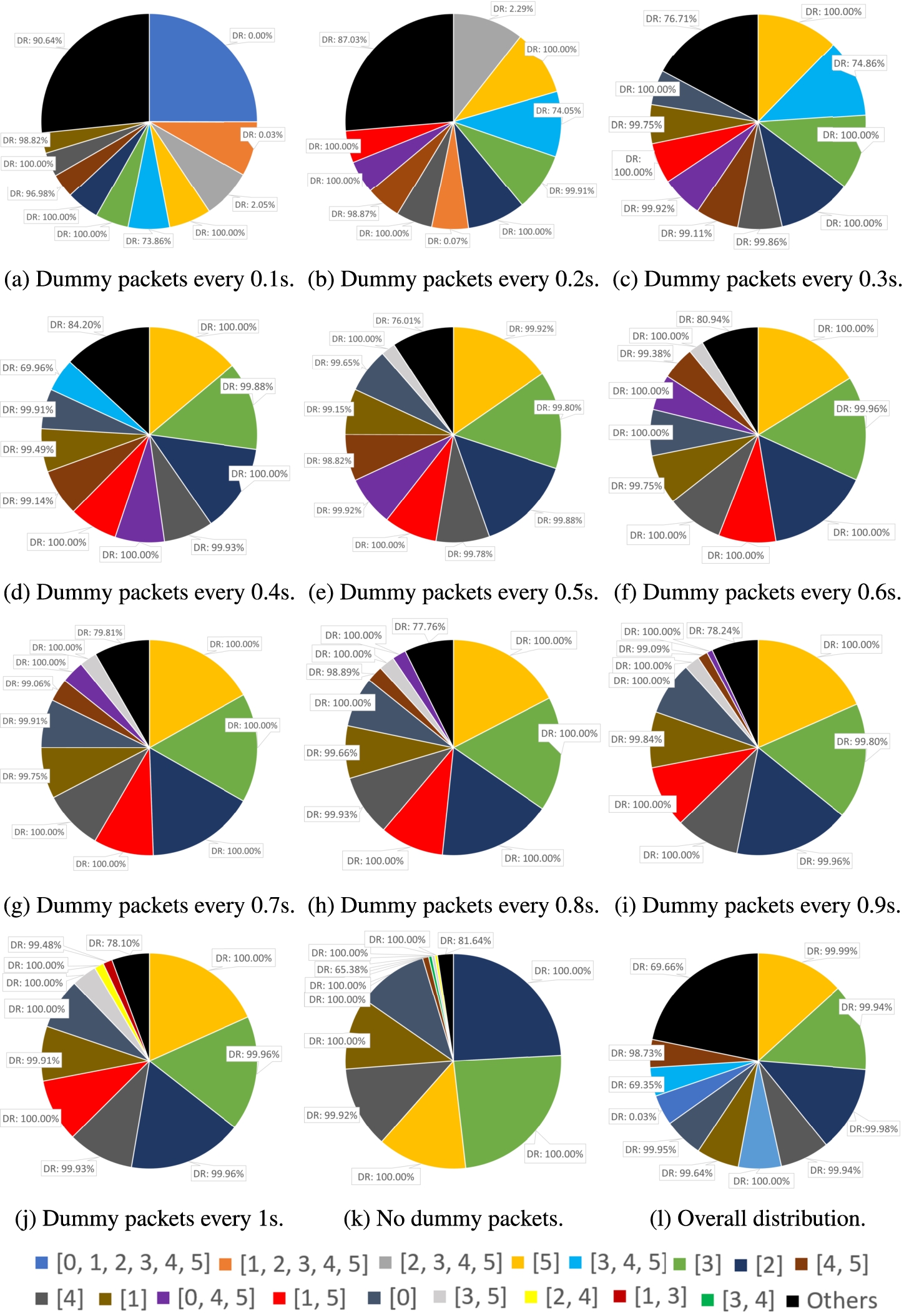
Detection Rates with respect to Attacker Packet Indices. We have conducted statistics and find that detection rates corresponding to different attacker packet indices are very polarized. Full results are shown in Fig. 8. Indices are shown with numbers. For example, $[0, 1, 2, 3, 4, 5]$ means that all 6 packets represented in the data sample are all attacker packets, and $[2, 3, 4, 5]$ means that the third, forth, fifth and sixth packets represented in the data samples are attacker packets. The majority of detection rates are above 90%; some are about 70%; and others are below 5%. None of them are between 5% to 65%.

Fig. 8.

Attacker packet index distributions and corresponding detection rates.

Generally speaking, less frequent dummy attack packets result in the high detection rates. For example, when dummy packets are sent out every 0.1 s, one-third (of 3 attacker packet indices or pies) of the data samples have DRs close to 0%; when the time interval is 0.2 s, the rate drops to about 10% (of just 1 attacker packet index or pie); when the time interval becomes greater than 0.2 s, the most common ten attacker packet indices all have high detection rate. In a word, the distribution of attacker packet indices is not a uniform distribution, different attacker packet indices have different DRs, and how frequently dummy attack packets are sent have a big influence on attacker packet index distribution.

Impact of Adversarial Value Set Selection. To build the dictionary that helps to select the suitable adversarial value set, we have conducted additional DNS cache poisoning attacks to collect data and generate PCAW adversarial examples with masked FGSM (Masked ZOO is too time-consuming, so it is not used here.) After launching the DNS cache poisoning attack for 60000 times with dummy attack packets, a total of 244340 data samples are generated, which result in a dictionary with 148 keys holding 202 adversarial value sets.

We tried all the distance measuring methods mentioned in Section 5.4, and experiment results are summarized in Table 8. Each row shows results for one method (with 5000 attack sessions conducted for each method respectively), and each column shows the detection rates with respect to the number of attack packets represented in one data sample. The last column shows the average numbers of represented attack packets and the average detection rates. Similar to Table 6, the more attack packets represented in one data sample, the less likely the attack can be detected. When no dummy attack packets are sent out, DRs are almost 100%. When dummy attack packets are used, 1) $L_{1}$ and $L_{2}$ distance measuring methods fail to decrease detection rates, while $L_{0}$ and $L_{inf}$ succeed in decreasing detection rates; 2) $L_{0}$ distance measuring achieves the lowest detection rates. Comparing to “random with dummy”, the detection rate drops from 79.84% to 66.02%.

Table 8

Detection rates with respect to the number of different distance measuring methods

Type	Number of attack packets represented in each data samples						Average

	1	2	3	4	5	6

	DR	DR	DR	DR	DR	DR	DR
Random¹	99.99%	100.00%	–				99.99%
Random¹ with dummy²	99.72%	98.87%	90.33%	39.51%	18.72%	8.80%	79.84%
$L_{0}$	99.99%	100.00%	–				99.99%
$L_{0}$ with dummy²	99.73%	95.58%	58.37%	4.73%	0.24%	0.28%	66.02%
$L_{1}$	100.00%	100.00%	–				100.00%
$L_{1}$ with dummy²	99.77%	98.73%	82.54%	46.63%	39.23%	26.27%	81.30%
$L_{2}$	100.00%	100.00%	–				100.00%
$L_{2}$ with dummy²	99.80%	98.91%	81.77%	47.50%	38.16%	28.80%	80.69%
$L_{inf}$	100.00%	100.00%	–				100.00%
$L_{inf}$ with dummy²	99.78%	98.13%	72.19%	9.63%	0.12%	0.00%	69.12%

¹ “Random” means the dictionary is not used and adversarial value sets are selected totally randomly. The two “random” cases serve as the baselines. ² Dummy attack packets, if used, are sent out every 0.1 s.

In addition to the data sample level, we have also inspected the collected data on the session level. To our surprise, the results show that none of the sessions in the ten cases shown in Table 8 are stealthy attack sessions, which probably means they can all be detected. This indicates that though adversarial value set selection can effectively lower the DRs at data sample level on general, it is not effective at the session level. A closer look at the sessions and the data samples also shows that, it is usually the first several data samples in the session that cannot get misclassified. Such data samples have only 1 or 2 attack packets inside. The reason is that the local DNS server, on receiving the user machine’s query packet, will send out several packets successively: query the IP address of the desired domain name, query the authoritative DNS server, query the IP addresses of root DNS servers, etc. As a result, every session is certain to have data samples that have very few attack packets, and the DR on the session level cannot be effectively lowered.

Phase 3: Launching stealthy DNS cache poisoning attacks.

We build an adversarial value set database with the two stealthy attack sessions we found, and use it to simulate a patient and cautious attacker. If the attacker takes no action in a DNS session, it is referred as a “no-attack session”; if the attacker takes some action(s), but aborts before the attack is finished and does not fully replay the template session, it is referred as an “aborted session”; if the attacker fully replays the template session, it is referred as a “replayed session”. In our experiment, it takes about four days with 46545 DNS sessions, to get a perfect attack chance. The 46545 DNS sessions contains 46541 no-attack sessions, 3 aborted sessions, and the last one replayed session. We have also verified that none of the no-attack sessions are reported as false positive; all aborted sessions are correctly detected as malicious (stealthy attack session is not fully replayed, so aborted sessions cannot guarantee to be stealthy); for the one replayed session, it is not detected, and the attack succeeds.

Though it seems that a perfect chance is hard to wait, considering that attackers can even wait for months to take actions in APT campaigns, we believe several days is realistic and acceptable for attackers. To provide an estimation of the waiting time, we have the following observation: 1) in a large-scale enterprise network, a typical local DNS server’s network throughput is about 6 Mbps, namely $6 * 1024 * 1024 / 8$ bytes per second. 2) Half of all the local DNS server’s network traffic is DNS traffic. 3) An average DNS packet is 170 bytes in length. 4) A DNS session, if the entry is already cached (no attack chance), can be as short as 2 packets; if the entry is not cached (potential attack chance) and attackers are not involved, the session can contain at least 4 packets; or, if the attacker launched the DNS cache poisoning attack, the session can be even longer (not to mention if dummy attack packets are used). In the worst case, we assume that every DNS session, on average, contains 12 packets, which means $6 * 1024 * 1024 / 8 / 2 / 170 / 12 \approx 193$ sessions per second. Therefore, even if there are as few as one potential attack chance out of 1000 DNS sessions, every $1000 / 386 \approx 5.181$ seconds, there will be one attack chance. Considering the results in the previous paragraph, every $5.181 seconds * 46545 \approx 67 hours$ , attackers can expect one successful stealthy DNS cache poisoning attack. Also, our results are achieved with a database containing two stealthy attack sessions. If the attacker invests more time and efforts for preparations, and builds the database with more stealthy attack sessions, the estimated waiting time can be further shortened.

6.3. Q3: Costs of the proposed methods

Time and Memory Consumption. When generating PCAW adversarial examples, we also monitor the time and memory consumption. Memory consumption is measured by computing the memory usage increase caused by the PCAW adversarial example generation. From Table 4, it can be observed that masked FGSM needs exceptionally less time, but tends to have more memory consumption than masked ZOO. Masked random uses the most time and memory, because it is designed to loop until an adversarial example is found, or the algorithm reaches the maximum iterations. Compared to FGSM and ZOO, the random method does not have any guideline to generate perturbations, so it becomes the most inefficient approach.

PCAW Adversarial Examples’ Losses. In the area of adversarial learning, losses measure the distance of adversarial examples to their seed data samples, which indicate to what extent a data sample has to be modified so that it becomes an adversarial example. Assuming $x_{i j}$ represents a feature in the seed data sample, and $x_{i j}^{'}$ represents a feature in the adversarial example, we use the similar distance measuring methods $L_{0}$ , $L_{1}$ , $L_{2}$ , and $L_{inf}$ mentioned earlier. We have measured the average losses of our generated PCAW adversarial examples, as presented in Table 9. For ARP poisoning, no PCAW adversarial examples are generated with masked FGSM, so losses are only calculated for those generated by masked ZOO. The $L_{0}$ average loss is 11, $L_{1}$ is 1214.17, $L_{2}$ is 418.43, and $L_{inf}$ is 210.67. It means that about 11 bytes ( $L_{0}$ ) in the ARP packets need to be modified, and the values ( $L_{inf}$ ) may be changed by 210.67. For DNS cache poisoning, depending on how many attack packets are represented in the data sample, how large the changeable portion varies, so they are listed separately. If there is only one attack packet represented, no PCAW adversarial examples are generated, so losses cannot be calculated. If there are two attack packets represented, masked FGSM can generate PCAW adversarial examples with relatively few modifications. The $L_{0}$ average loss is 18.33, $L_{1}$ is 18.33, $L_{2}$ is 4.26, and $L_{inf}$ is 1. Because every feature for data samples of DNS poisoning detection is either 0 or 1, $L_{0} = = L_{1}$ , and $L_{inf}$ can only be 0 or 1.

Table 9
PCAW adversarial examples’ average losses

Attack Measurements Masked FGSM Masked ZOO

ARP $L_{0}$ -^* 11

$L_{1}$ 1214.17

$L_{2}$ 418.43

$L_{inf}$ 210.67

DNS $L_{0}$ -^*

(one attack $L_{1}$

packet in $L_{2}$

data sample) $L_{inf}$

DNS $L_{0}$ 18.33 23.83

(two attack $L_{1}$ 18.33 23.83

packets in $L_{2}$ 4.26 4.87

data sample) $L_{inf}$ 1 1

Attack	Measurements	Masked FGSM	Masked ZOO
ARP	$L_{0}$	-^*	11
	$L_{1}$	1214.17
	$L_{2}$	418.43
	$L_{inf}$	210.67
DNS	$L_{0}$	-^*
(one attack	$L_{1}$
packet in	$L_{2}$
data sample)	$L_{inf}$
DNS	$L_{0}$	18.33	23.83
(two attack	$L_{1}$	18.33	23.83
packets in	$L_{2}$	4.26	4.87
data sample)	$L_{inf}$	1	1

^* Some results cannot be presented because there are no PCAW adversarial examples in those cases, and losses cannot be calculated.

7. Discussion

7.1. Limitations

Attack success rates and stealthiness are usually the top concerns of attackers, especially for the ones conducting Advanced Persistent Threats (APTs).

We have proposed new evasion methods to generate malicious adversarial examples, so that attack success rate and stealthiness are both preserved. However, as shown in Section 6, they are not very efficient. For network attacks that need multiple network packets to launch and detect, such as DNS cache poisoning, sending dummy attacker packets is an effective way to substantially decrease the chances of being detected by neural networks. Nevertheless, dummy packets can also increase the attackers’ risks of being noticed due to the abnormal packet contents and the increased interaction with the target machines or servers.

Therefore, it is very challenging for attackers to find a perfect solution that can preserve network attack success rate, stealthiness, and efficiency all at once. Attackers will need to make trade-offs among these aspects. PCAW adversarial examples can be pre-generated, so that the attacker can quickly refer to them and send out attack packets when launching real attacks. Nevertheless, the attacker still needs to invest lots of time and effort to gather data and generate PCAW adversarial examples (and to mitigate uncertainties for multi-packet network attacks). We identify those as necessary costs to the attacker. As for defenders, it is recommended to combine multiple detection approaches rather than just using one, such as outlier detectors.

7.2. Counter measures

The previous sections presented a novel attack type with PCAWAEs. This attack is stealthier than traditional network attacks and can still result in the malicious impact. What is more, because attackers modify the contents of the packets, network flow-based IDS may not be effective detecting this attack. However, because the PCAWAE generation is still based on observed adversarial example generation methods, PCAWAE may be rejected if adversarial learning techniques are applied.

This paper focuses on the attacking aspect, so we will only briefly discuss the counter measures. Generally speaking, adversarial learning techniques can be categorized based on the time point of deployment [57]: before or after the original model is produced. Some common adversarial learning techniques include adversarial training [16], where adversarial examples are augmented into the training data to train a robust model, defensive distillation [38], where a separate model is learned based on the output of a previous model, and data compression [13], where the original data samples are compressed to mitigate the effect of attacker perturbations. However, adversarial training needs a lot of adversarial examples. In our case, they should be PCAWAEs, which are not easy to generate. Defensive distillation does not need adversarial examples as input, but it is not effective against some advanced attacks [8,9]. Unlike images, data compression may break some intrinsic patterns within network packet data. Therefore, instead of the above-mentioned common techniques, we select DeepCloak [15], which adds a mask layer just before the output layer of the detection model, so that extracted features that are affected by adversarial examples most will be filtered out.

We applied DeepCloak to the ARP poisoning detection neural network. As shown in Fig. 1, the output layer contains 2 units for binary classification, and there are 35 extracted features from the previous layer. Our experiment results show that, when 1 extracted feature is filtered out, out of the 36 PCAWAEs generated by masked ZOO, 33 of them are now correctly predicted as malicious, and changes to the evaluation metrics (accuracy, recall, precision, and F1 score) on the original dataset is about 0.0001. We continue to increase the number of filtered out extracted features, and find out that the maximum number of reverted PCAWAEs is 34. When the number of filtered out extracted features is nearing half of all extracted features, the model’s evaluation metrics will decrease drastically. In conclusion, though DeepCloak may not be able to revert all PCAWAEs’ predicted labels to the correct labels, it is still an effective defense approach because it can revert about 90% of the PCAWAEs’ predicted labels.

8. Related work

In the domain of network security, all the existing work on generating adversarial examples are under the data manipulation threat model. In particular, we break them down into two groups.

Packet content manipulation. In [17] and [49], the authors show how a NN-based detector which works on network flow data can be evaded. In [17], the original malicious network traffic is mutated to transfer its features to the closest adversarial ones, and the authors used a special distance metric between two feature vectors to help solve the corresponding bi-level optimization problem. However, because no network/protocol constraint is considered in solving the optimization problem, the generated adversarial examples are not protocol-constraint-aware.

In [49], the authors conducted systematic experiments to evaluate whether the generated adversarial examples can evade the NN-based detectors. However, since the data manipulation threat model is assumed in this study, the authors did not propose any method for using the generated adversarial examples to generate the adversarial attack packets. Without these adversarial attack packets, the authors did not launch any real network attacks in their experiments. Another main difference between [49] and our work is as follows: the network constraints considered in [17,49] focus on transport layer protocols (e.g., TCP and UDP); in contrast, because we aim to launch real network attacks under the standard threat model, the protocol constraints considered in our work are specific to individual attacks. For example, for the DNS cache poisoning attack, we focus on the constraints specific to the DNS protocol.

Another work [41] proposes to modify packets themselves, but it only pads the packets with redundant bits, making the packets in question easy to be filtered out and noticed by security operators.

Timing manipulation and packet injection. The work conducted in [18] assumes that attackers can split large Transmission Control Protocol (TCP) data (to be sent) into multiple smaller packets, and generates adversarial examples by maliciously (a) manipulating the timing for sending out packets and (b) injecting fake packets. Note that our approach neither manipulates timing information, nor injects any fake packets.

9. Conclusion

With deep-learning-based detection systems being increasingly deployed in enterprise networks, if the adversary continues to launch network attacks (as usual) without any adjustment, their APT campaigns would become significantly less stealthy. Noticing that none of the existing adversarial example generation methods could generate malicious packets that can simultaneously compromise the target machine and evade the neural network detection model, we introduced a practical way for launching stealthy network attacks, and proposed the approach of implementing this type of attack. We used ARP poisoning and DNS cache poisoning attacks as the case study to demonstrate the effectiveness of the proposed method.

Disclaimer

Dr. Liu and The Pennsylvania State University own equity in DayZero Systems. These financial interests have been reviewed by the University’s Conflict of Interest Committees and are currently being managed by the University.

This paper is not subject to copyright in the United States. Commercial products are identified in order to adequately specify certain procedures. In no case does such identification imply recommendation or endorsement by the National Institute of Standards and Technology, nor does it imply that the identified products are necessarily the best available for the purpose.

Footnotes

Acknowledgment

This work was supported by NIST 60NANB22D144, NSF CNS-2019340, and NSF ECCS-2140175. Xiaoyan Sun was supported by NSF DGE-2105801.

References

Alzantot,

Sharma,

Chakraborty,

Zhang,

C.-J.

Hsieh and

Srivastava, GenAttack: Practical Black-box Attacks with Gradient-Free Optimization, 2019, arXiv:1805.11090 [cs].

Apruzzese,

Andreolini,

Ferretti,

Marchetti and

Colajanni, Modeling realistic adversarial attacks against network intrusion detection systems, Digital Threats 3(3) (2022). doi:10.1145/3469659.

Apruzzese,

Colajanni and

Marchetti, Evaluating the effectiveness of adversarial attacks against botnet detectors, in: 2019 IEEE 18th International Symposium on Network Computing and Applications (NCA), 2019, pp. 1–8, ISSN 2643-7929. doi:10.1109/NCA.2019.8935039.

Apruzzese,

Vladimirov,

Tastemirova and

Laskov, Wild networks: Exposure of 5G network infrastructures to adversarial examples, IEEE Transactions on Network and Service Management 19(4) (2022), 5312–5332. doi:10.1109/TNSM.2022.3188930.

Artificial Intelligence (AI) for Cybersecurity | IBM, 2023, [Online; accessed 27. Jun. 2023]. https://www.ibm.com/security/artificial-intelligence?utm_content=SRCWW&p1=Search&p4=43700074604519875&p5=p&gclsrc=aw.ds.

Brendel,

Rauber and

Bethge, Decision-Based Adversarial Attacks: Reliable Attacks Against Black-Box Machine Learning Models, 2018, arXiv:1712.04248.

Brendel,

Rauber,

Kümmerer,

Ustyuzhaninov and

Bethge, Accurate, reliable and fast robustness evaluation, 2019, arXiv:1907.01003.

Carlini and

Wagner, Defensive distillation is not robust to adversarial examples, 2016, arXiv preprint arXiv:1607.04311.

Carlini and

Wagner, Towards evaluating the robustness of neural networks, in: 2017 IEEE Symposium on Security and Privacy (SP), 2017, pp. 39–57, ISSN 2375-1207. doi:10.1109/SP.2017.49.

10.

Chen,

M.I.

Jordan and

M.J.

Wainwright, HopSkipJumpAttack: A query-efficient decision-based attack, in: 2020 IEEE Symposium on Security and Privacy (SP), 2020, pp. 1277–1294, ISSN 2375-1207. doi:10.1109/SP40000.2020.00045.

11.

P.-Y.

Chen,

Sharma,

Zhang,

Yi and

C.-J.

Hsieh, EAD: Elastic-net attacks to deep neural networks via adversarial examples, in: Proceedings of the AAAI Conference on Artificial Intelligence 32(11), 2018, https://ojs.aaai.org/index.php/AAAI/article/view/11302 .

12.

P.-Y.

Chen,

Zhang,

Sharma,

Yi and

C.-J.

Hsieh, ZOO: Zeroth order optimization based black-box attacks to deep neural networks without training substitute models, in: Proceedings of the 10th ACM Workshop on Artificial Intelligence and Security, AISec’17, Association for Computing Machinery, 2017, pp. 15–26. ISBN 978-1-4503-5202-4. doi:10.1145/3128572.3140448.

13.

G.K.

Dziugaite,

Ghahramani and

D.M.

Roy, A study of the effect of jpg compression on adversarial images, 2016, arXiv preprint arXiv:1608.00853.

14.

Fortinet Introduces Self-Learning Artificial Intelligence Appliance for Sub-Second Threat Detection, 2021, [Online; accessed 15. Jun. 2021]. https://www.fortinet.com/corporate/about-us/newsroom/press-releases/2020/introduces-self-learning-artificial-intelligence-appliance-for-sub-2nd-threat-detection.

15.

Gao,

Wang,

Lin,

Xu and

Qi, DeepCloak: Masking Deep Neural Network Models for Robustness Against Adversarial Samples, 2017, arXiv:1702.06763 [cs]. doi:10.48550/arXiv.1702.06763.

16.

I.J.

Goodfellow,

Shlens and

Szegedy, Explaining and harnessing adversarial examples, 2014, arXiv preprint arXiv:1412.6572.

17.

Han,

Wang,

Zhong,

Chen,

Yang,

Lu,

Shi and

Yin, Evaluating and improving adversarial robustness of machine learning-based network intrusion detectors, IEEE Journal on Selected Areas in Communications 39(8) (2021), 2632–2647. doi:10.1109/JSAC.2021.3087242.

18.

M.J.

Hashemi,

Cusack and

Keller, Towards evaluation of NIDSs in adversarial setting, in: Big-DAMA’19, Association for Computing Machinery, New York, NY, USA, 2019, pp. 14–21. ISBN 978-1-4503-6999-2. doi:10.1145/3359992.3366642.

19.

Home – Suricata, 2021, [Online; accessed 15. Jun. 2021]. https://suricata.io.

20.

M.D.

Hossain,

Ochiai,

Fall and

Kadobayashi, LSTM-based network attack detection: Performance comparison by hyper-parameter values tuning, in: 2020 7th IEEE International Conference on Cyber Security and Cloud Computing (CSCloud)/2020 6th IEEE International Conference on Edge Computing and Scalable Cloud (EdgeCom), IEEE, 2020, pp. 62–69.

21.

Hosseini,

Xiao,

Jaiswal and

Poovendran, On the limitation of convolutional neural networks in recognizing negative images, in: 2017 16th IEEE International Conference on Machine Learning and Applications (ICMLA), 2017, pp. 352–358. doi:10.1109/ICMLA.2017.0-136.

22.

infosecdr, spade, 2021, [Online; accessed 15. Jun. 2021]. https://github.com/infosecdr/spade.

23.

Ingre,

Yadav and

A.K.

Soni, Decision tree based intrusion detection system for NSL-KDD dataset, in: Information and Communication Technology for Intelligent Systems (ICTIS 2017) –Volume 2 2, Springer, 2018, pp. 207–218.

24.

Jakkal, Empowering defenders at the speed of AI – The Official Microsoft Blog, Official Microsoft Blog (2023). https://blogs.microsoft.com/blog/2023/03/28/introducing-microsoft-security-copilot-empowering-defenders-at-the-speed-of-ai.

25.

Jang,

Wu and

Jha, Objective metrics and gradient descent algorithms for adversarial examples in machine learning, in: Proceedings of the 33rd Annual Computer Security Applications Conference, ACSAC 2017, Association for Computing Machinery, 2017, pp. 262–277. ISBN 978-1-4503-5345-8. doi:10.1145/3134600.3134635.

26.

Kokila,

S.T.

Selvi and

Govindarajan, DDoS Detection and Analysis in SDN-Based Environment Using Support Vector Machine Classifier, IEEE, 2014, pp. 205–210, in: 2014 sixth international conference on advanced computing (ICoAC).

27.

M.V.

Kotpalliwar and

Wajgi, Classification of attacks using support vector machine (svm) on kddcup’99 ids database, in: 2015 Fifth International Conference on Communication Systems and Network Technologies, IEEE, 2015, pp. 987–990. doi:10.1109/CSNT.2015.185.

28.

Kurakin,

Goodfellow and

Bengio, Adversarial Examples in the Physical World, 2017, arXiv:1607.02533.

29.

Madry,

Makelov,

Schmidt,

Tsipras and

Vladu, Towards deep learning models resistant to adversarial attacks, 2017, arXiv preprint arXiv:1706.06083.

30.

A.J.

Malik and

F.A.

Khan, A hybrid technique using binary particle swarm optimization and decision tree pruning for network intrusion detection, Cluster Computing 21 (2018), 667–680. doi:10.1007/s10586-017-0971-8.

31.

Mirsky,

Doitshman,

Elovici and

Shabtai, Kitsune: An ensemble of autoencoders for online network intrusion detection, 2018, arXiv:1802.09089 [cs]. doi:10.48550/arXiv.1802.09089.

32.

Miyato,

S.-I.

Maeda,

Koyama,

Nakae and

Ishii, Distributional Smoothing with Virtual Adversarial Training, 2016, arXiv:1507.00677.

33.

S.-M.

Moosavi-Dezfooli,

Fawzi and

Frossard, Deepfool: A simple and accurate method to fool deep neural networks, in: Proceedings of the IEEE Conference on Computer Vision and Pattern Recognition, 2016, pp. 2574–2582.

34.

M.-I.

Nicolae,

Sinn,

M.N.

Tran,

Buesser,

Rawat,

Wistuba,

Zantedeschi,

Baracaldo,

Chen,

Ludwig,

Molloy and

Edwards, Adversarial Robustness Toolbox v1.2.0, CoRR 1807 (2018), 01069, https://arxiv.org/pdf/1807.01069 .

35.

Papernot,

McDaniel and

Goodfellow, Transferability in machine learning: from phenomena to black-box attacks using adversarial samples, 2016, arXiv preprint arXiv:1605.07277.

36.

Papernot,

McDaniel,

Goodfellow,

Jha,

Z.B.

Celik and

Swami, Practical black-box attacks against machine learning, in: Proceedings of the 2017 ACM on Asia Conference on Computer and Communications Security, 2017, pp. 506–519. doi:10.1145/3052973.3053009.

37.

Papernot,

McDaniel,

Jha,

Fredrikson,

Z.B.

Celik and

Swami, The limitations of deep learning in adversarial settings, in: 2016 IEEE European Symposium on Security and Privacy (EuroS P), 2016, pp. 372–387. doi:10.1109/EuroSP.2016.36.

38.

Papernot,

McDaniel,

Wu,

Jha and

Swami, Distillation as a defense to adversarial perturbations against deep neural networks, in: 2016 IEEE Symposium on Security and Privacy (SP), IEEE, 2016, pp. 582–597. doi:10.1109/SP.2016.41.

39.

Pierazzi,

Pendlebury,

Cortellazzi and

Cavallaro, Intriguing properties of adversarial ML attacks in the problem space, in: 2020 IEEE Symposium on Security and Privacy (SP), 2020, pp. 1332–1349. doi:10.1109/SP40000.2020.00073.

40.

C.F.

Pontes,

M.M.

De Souza,

J.J.

Gondim,

Bishop and

M.A.

Marotta, A new method for flow-based network intrusion detection using the inverse Potts model, IEEE Transactions on Network and Service Management 18(2) (2021), 1125–1136. doi:10.1109/TNSM.2021.3075503.

41.

Qiu,

Dong,

Zhang,

Lu,

Memmi and

Qiu, Adversarial attacks against network intrusion detection in IoT systems, IEEE Internet of Things Journal 8(13) (2021), 10327–10335. doi:10.1109/JIOT.2020.3048038.

42.

B.B.

Rao and

Swathi, Fast kNN classifiers for network intrusion detection system, Indian Journal of Science and Technology 10(14) (2017), 1–10.

43.

Rauber,

Brendel and

Bethge, Foolbox: A Python toolbox to benchmark the robustness of machine learning models, in: Reliable Machine Learning in the Wild Workshop, 34th International Conference on Machine Learning, 2017, http://arxiv.org/abs/1707.04131 .

44.

Rauber,

Zimmermann,

Bethge and

Brendel, Foolbox native: Fast adversarial attacks to benchmark the robustness of machine learning models in PyTorch, TensorFlow, and JAX, Journal of Open Source Software 5(53) (2020), 2607. doi:10.21105/joss.02607.

45.

Revathi and

Malathi, A detailed analysis on NSL-KDD dataset using various machine learning techniques for intrusion detection, International Journal of Engineering Research & Technology (IJERT) 2(12) (2013), 1848–1853.

46.

Rony,

L.G.

Hafemann,

L.S.

Oliveira,

I.B.

Ayed,

Sabourin and

Granger, Decoupling direction and norm for efficient gradient-based L2 adversarial attacks and defenses, 2019, arXiv:1811.09600 [cs].

47.

A.M.

Sharifi,

S.K.

Amirgholipour and

Pourebrahimi, Intrusion detection based on joint of k-means and knn, Journal of Convergence Information Technology 10(5) (2015), 42.

48.

Sheatsley,

Hoak,

Pauley,

Beugin,

M.J.

Weisman and

McDaniel, On the robustness of domain constraints, in: Proceedings of the 2021 ACM SIGSAC Conference on Computer and Communications Security, CCS’21, Association for Computing Machinery, New York, NY, USA, 2021, pp. 495–515. ISBN 9781450384544. doi:10.1145/3460120.3484570.

49.

Sheatsley,

Papernot,

M.J.

Weisman,

Verma and

McDaniel, Adversarial examples for network intrusion detection systems, Journal of Computer Security 30(5) (2022), 727–752. doi:10.3233/JCS-210094.

50.

Snort – Network Intrusion Detection & Prevention System, 2021, [Online; accessed 15. Jun. 2021]. https://www.snort.org.

51.

Splunk and Tensorflow for Security: Catching the Fraudster with Behavior Biometrics, 2017, [Online; accessed 15. Jun. 2021]. https://www.splunk.com/en_us/blog/security/deep-learning-with-splunk-and-tensorflow-for-security-catching-the-fraudster-in-neural-networks-with-behavioral-biometrics.html.

52.

Tavallaee,

Bagheri,

Lu and

A.A.

Ghorbani, A detailed analysis of the KDD CUP 99 data set, in: 2009 IEEE Symposium on Computational Intelligence for Security and Defense Applications, Ieee, 2009, pp. 1–6.

53.

The Zeek Network Security Monitor, 2023, [Online; accessed 21. Feb. 2023]. https://zeek.org.

54.

Townsend, SaaS Ransomware Attack Hit Sharepoint Online Without Using a Compromised Endpoint, SecurityWeek (2023), https://www.securityweek.com/saas-ransomware-attack-hit-sharepoint-online-without-using-a-compromised-endpoint.

55.

Training Transformers for Cyber Security Tasks: A Case Study on, 2021, [Online; accessed 15. Jun. 2021]. https://www.fireeye.com/blog/threat-research/2021/01/training-transformers-for-cyber-security-tasks-malicious-url-prediction.html.

56.

Tramèr and

Boneh, Adversarial Training and Robustness for Multiple Perturbations, 2019, arXiv:1904.13000.

57.

Wang,

Li,

Kuang,

Y.-A.

Tan and

Li, The security of machine learning in an adversarial setting: A survey, Journal of Parallel and Distributed Computing 130 (2019), 12–23. doi:10.1016/j.jpdc.2019.03.003.

58.

Wu,

Fang,

Wang,

Liu and

Cui, Evading machine learning botnet detection models via deep reinforcement learning, in: ICC 2019–2019 IEEE International Conference on Communications (ICC), 2019, pp. 1–6. doi:10.1109/ICC.2019.8761337.

59.

Yuan,

He,

Zhu and

Li, Adversarial examples: Attacks and defenses for deep learning, IEEE transactions on neural networks and learning systems 30(9) (2019), 2805–2824. doi:10.1109/TNNLS.2018.2886017.

60.

Yuan,

Li and

Li, DeepDefense: Identifying DDoS Attack via Deep Learning, in: 2017 IEEE International Conference on Smart Computing, SMARTCOMP 2017, 2017, https://ieeexplore.ieee.org/abstract/document/7946998/ .

61.

Zhang,

Chen,

Guo,

Song,

Teng and

Wang, PCCN: Parallel cross convolutional neural network for abnormal network traffic flows detection in multi-class imbalanced network traffic flows, IEEE Access (2019), 1–1, https://ieeexplore.ieee.org/abstract/document/8787567/.

62.

Zou,

Singhal,

Sun and

Liu, Deep learning for detecting logic-flaw-exploiting network attacks: An end-to-end approach, Journal of Computer Security (2021), 1–30.

Analysis of neural network detectors for network attacks

Abstract

Keywords

1. Introduction

2. Background and motivation

2.1. Network attacks and NIDS

2.2. ML-based network attack detectors

2.3. Adversarial examples for DNNs

2.4. Why the adversarial examples generated by existing methods fail under the standard threat model

Table 2 Dataset statistics Attacks Set Size Benign to malicious ratio ARP poisoning Training 9584 1.005:1 Test 2400 0.982:1 DNS cache poisoning Training 30928 1.003:1 Test 7732 0.988:1

4.1. Protocol-constraint-AWare adversarial examples

4.2. Unique challenges in multi-packet stealthy network attacks

5. Proposed stealthy adversarial attacks

5.1. Work flow of stealthy network attacks

5.4. Mitigate uncertainties for multi-packet attacks

6.1. Q1: Stealthy ARP poisoning

7.1. Limitations

7.2. Counter measures

8. Related work

9. Conclusion

Disclaimer

Footnotes

Acknowledgment

References

Table 2
Dataset statistics

Attacks Set Size Benign to malicious ratio

ARP poisoning Training 9584 1.005:1

Test 2400 0.982:1

DNS cache poisoning Training 30928 1.003:1

Test 7732 0.988:1