Labour income inequality in Mexico: Puzzles solved and unsolved

Abstract

We analyse the evolution and proximate determinants of labour income inequality in Mexico between 1989 and 2017. Labour income inequality increased between 1989 and 1994 and declined between 1994 and 2006. What happened after 2006 is subject to uncertainty. The national labour force survey shows a steady decline and the income expenditure survey suggests that inequality increased. We correct for high and rising item (labour income) non-response and under-representation of high-wage earners through a ‘hot deck’ imputation method and, for workers in the formal sector, through post-survey weight adjustments. We obtain the new weights for formal workers from tabulations recently released by the Mexican social security administration. With corrected data, inequality no longer declines between 2006 and 2017.

Keywords

Inequality labour income post-survey reweighting imputation decomposition methods Mexico

1. Introduction

Partly as a result of rising inequality in a number countries, the accurate measurement of inequality has gained a lot of attention from academics and policymakers. This has resulted in a large body of literature on inequality dynamics in advanced countries and emerging economies, including Mexico. The interest in inequality dynamics in Mexico is particularly strong because it was among the first developing countries to introduce market-oriented structural reforms in the 1980s and 1990s. Among the leading reforms was the country’s opening up to external competition through ambitious trade liberalization in the 1980s. As part of this openness drive, Mexico joined Canada and the US in signing the North American Free Trade Agreement (NAFTA) in 1994. At the time the agreement was signed, NAFTA opponents were concerned with low wages and high inequality in Mexico because of their potential negative impact on US workers. Supporters argued that integration with the US would actually increase real wages in Mexico, especially at the lower end. As a result, the interest on what occurred to inequality, especially labour income inequality, in Mexico during the post-NAFTA era became even stronger. Hence the importance of having reliable data. Unfortunately, as this article shows, due to rising item nonresponse especially in labour surveys and undercoverage of high-wage workers in the upper tail, measuring labour income inequality with accuracy has become increasingly challenging. To address these two issues, here we implement a combination of imputation and post-survey weight adjustment methods and compute a new labour income inequality series with the corrected data. The challenge, however, remains because depending on whether one uses the labour survey or the household survey, after 2006 the inequality trends produced by each are still qualitatively different.

Today, Mexico is an upper-middle-income country with high levels of labour income inequality: in 2014, the Gini coefficient was in the range of 0.45 to 0.52 (depending on the source).1 In the last thirty years, its labour force became considerably more educated: the proportion of individuals with primary education or less rose from 67 percent in 1990 to 33 percent in 2015; and the proportion of individuals with a college education more than doubled between 1990 and 2015, when it reached around 15 percent. With the advent of digitalization, the last thirty years also witnessed sweeping changes in production technologies. In the light of these deve-lopments, how did labour income inequality change? We find that between the late 1980s and 1994, inequality increased (Fig. 1). This increase was driven, primarily, by an increase in the skill premium (returns to education, in particular) associated with higher demand for skills and falling minimum wages and unionization rates. After NAFTA came into effect (1994) and up to the mid-2000s, labour income inequality declined. In stark contrast with the earlier period, the skill premium fell. Since institutional factors such as the minimum wage and the unionization rate remained constant, the fall in the skill premium was associated with the fact that the supply of skilled workers outpaced demand (see for example [1, 2, 3]).

Figure 1.

Gini coefficient for labour income: 1989–2017 (ENOE, ENOE-urban, and ENIGH). Notes: Workers aged 20–64 years and with positive labour income and working hours. For ENOE we use the second quarter of each year. We exclude households whose head reports zero monetary income. ENOE-Urban restricted to urban municipalities (at least 100,000 inhabitants). Source: Authors’ construction.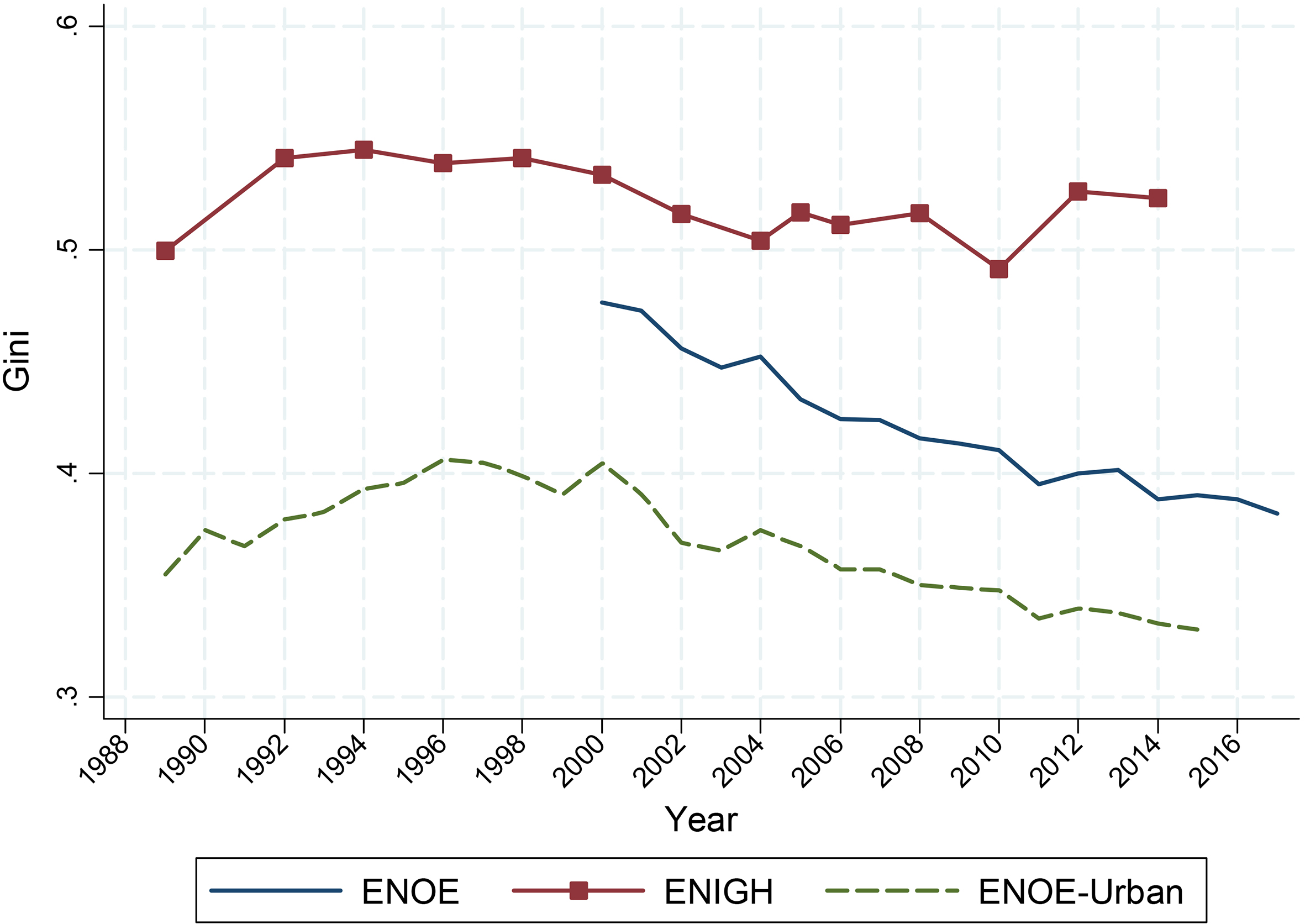

After 2006, however, the evolution of labour income inequality is far from clear due, in particular, to rising item nonresponse but also to the undercoverage of high-wage workers in the upper tail (see Fig. 1; all calculations were implemented in Stata v. 15, Windows 64). According to the Mexican labour force survey (herein ENOE, the Spanish acronym), labour income inequality continued its steady decline: the Gini coefficient went from 0.424 in 2006 to 0.382 in 2017. However, the Household Income Expenditure National Survey (herein ENIGH, the Spanish acronym) shows a slight increase: the Gini coefficient went from 0.511 in 2006 to 0.523 in 2014. Which of the two is correct? A serious problem with the labour force survey is that labour income (item) non-response (did not answer question on labour income) is high; and it steadily increased from 2006, reaching about a third of all workers (both formal and informal) by 2017. To deal with item nonresponse, we estimate the missing labour incomes by applying the so-called ‘hot deck’ imputation method, as proposed by [5]. In order to address the undercoverage of high-wage earners, we rely on recently released administrative data to carry out a post-survey weight adjustment to equate the distribution of workers by category in the survey to that observed in the administrative source (assumed to be the ‘true’ distribution).2 Since we do not have an external administrative source to generate ‘true’ weights for the informal sector workers, no such reweighting is applied to this group. Inequality estimates based on the corrected labour force survey ENOE no longer shows a steady decline: the Gini coefficient in both 2006 and 2017 is equal to 0.464. In sum, the evolution of inequality in the period after 2006 remains a bit ambiguous. The most one can say with certainty is that labour income inequality did not continue to decline.

Research shows that in Mexico changes in labour income inequality can be largely linked to changes in the relative wage between skilled and unskilled workers, that is, in the returns to skill. In particular, the rise in inequality during this period was associated with an increase in returns to schooling.3 Applying the RIF method proposed by [12] and the Oaxaca-Blinder decomposition method [11], show that the increase in earnings inequality between 1989 and 1994 is primarily driven by a rise in the returns to characteristics (schooling and experience). The effect of changes in the distribution of characteristics was almost flat. Using the framework proposed by [13], [11] conclude that both institutional factors and, surprisingly, the increase in relative demand for skilled workers (workers with high-school education and more) explained the increase in hourly wage inequality between 1989 and 1994. Hence, a key question is why demand for higher-educated individuals increased at a time when the Stolper-Samuelson theorem would have predicted the opposite.

The decline in earnings inequality between 1994 and 2006 is primarily driven by a fall in the returns to characteristics (schooling and experience). The effect of changes in the distribution of characteristics (education, experience, female and urban) was unequalizing. In other words, if the returns to characteristics had remained unchanged in this period, the change in characteristics in the population would have resulted in higher levels of inequality. Why were changes in characteristics unequalizing during a period in which there was substantial educational upgrading and the distribution of years of schooling became more equal? This seemingly contradictory result is a mathematical consequence of increasing returns to skill and was first noted by [14], who called it the ‘paradox of progress’.

[11] show that the change in the skill premium during this period is the result of a combination of a rising supply of workers with college education and a slow-down in demand for skilled workers.4 After 1996 the real minimum wage and the unionization rate were fairly stable. Hence, these key institutional factors could not explain the decline in returns. Behind the latter is the effect of the post-NAFTA intensification of integration with the United States, which has favoured the relatively low-skill sectors. As for the period after 2006, with corrected data, inequality no longer declines between 2006 and 2017.

The paper is organized as follows. Section 2 describes the data and the methods used to correct for item non-response and under-representation. Section 3 analyses the evolution of inequality with corrected data. Section 4 concludes.

2. Data and data corrections

Research on labour income dynamics usually relies on labour force surveys such as the Current Population Survey in the USA. Labour force surveys contain detailed information on employment, unemployment, hourly wages, self-employment income, and sociodemographic characteristics in a sample that is large enough for the study of patterns by sociodemographic characteristics, regions, and so on. However, in Mexico, the labour force survey reached national coverage only in 2000; before that, it covered urban areas only.5 Thus, for the analysis between 1989 and 2000, we rely entirely on ENIGH.

2.1 ENIGH, ENOE, and rising item non-response and undercoverage of high-wage earners

ENIGH is available for 1984 and 1989, at intervals of two years between 1992 and 2014, and also for 2005. The survey includes detailed information on income measures (wages and salaries, self-employed income, interests, rents, dividends, transfers, remittances, and income from other sources), sociodemographic characteristics of household members (age, education, gender, education), and expenditures by type, wealth, and assets at the household level. However, the methodology used to gene-rate labour income was modified in 2006, which creates challenges for comparisons over time,6 and this is one of the reasons we carry out the analysis for the period after that year separately. The labour income measure from ENIGH that we use in this paper includes wage and self-employment earnings, in both the formal and informal sectors.7 ENIGH is publicly available and can be downloaded from the website of the Mexican Statistical Office (INEGI, www.inegi.org.mx/).

From 2000 onwards, our analysis uses both ENIGH and ENOE. ENOE is a quarterly survey of over 100,000 households (see Table A2 in the supplementary materials) that follows the same household for five consecutive quarters. ENOE is used to calculate total employment, unemployment rates, and other labour market outcome characteristics at the national and state levels. In general, the methodology used to generate these surveys has remained largely the same, but the sampling has changed, as have some parts of the questionnaire. In particular, in 2005, ENOE was modified to homogenize the sociodemographic questionnaire with other surveys and to measure more precisely job search and employment duration. This year roughly coincides with the change in ENIGH mentioned above, so in both surveys it makes sense to do the analysis from 2006 onwards separately from before. As we shall see below, the year 2006 also (roughly) coincides with the point at which the decline in labour income inequality that had started in the mid-1990s stopped (ENOE is also publicly available and can be downloaded from the INEGI website).

Figure 2.

Workers with item non-response for labour income: 1988–2017 (ENOE and ENIGH; in % of total workers). Notes: Sample restricted to workers aged 20–64 years with positive labour income and working hours. For ENOE we use the second quarter of each year. Source: Authors’ construction.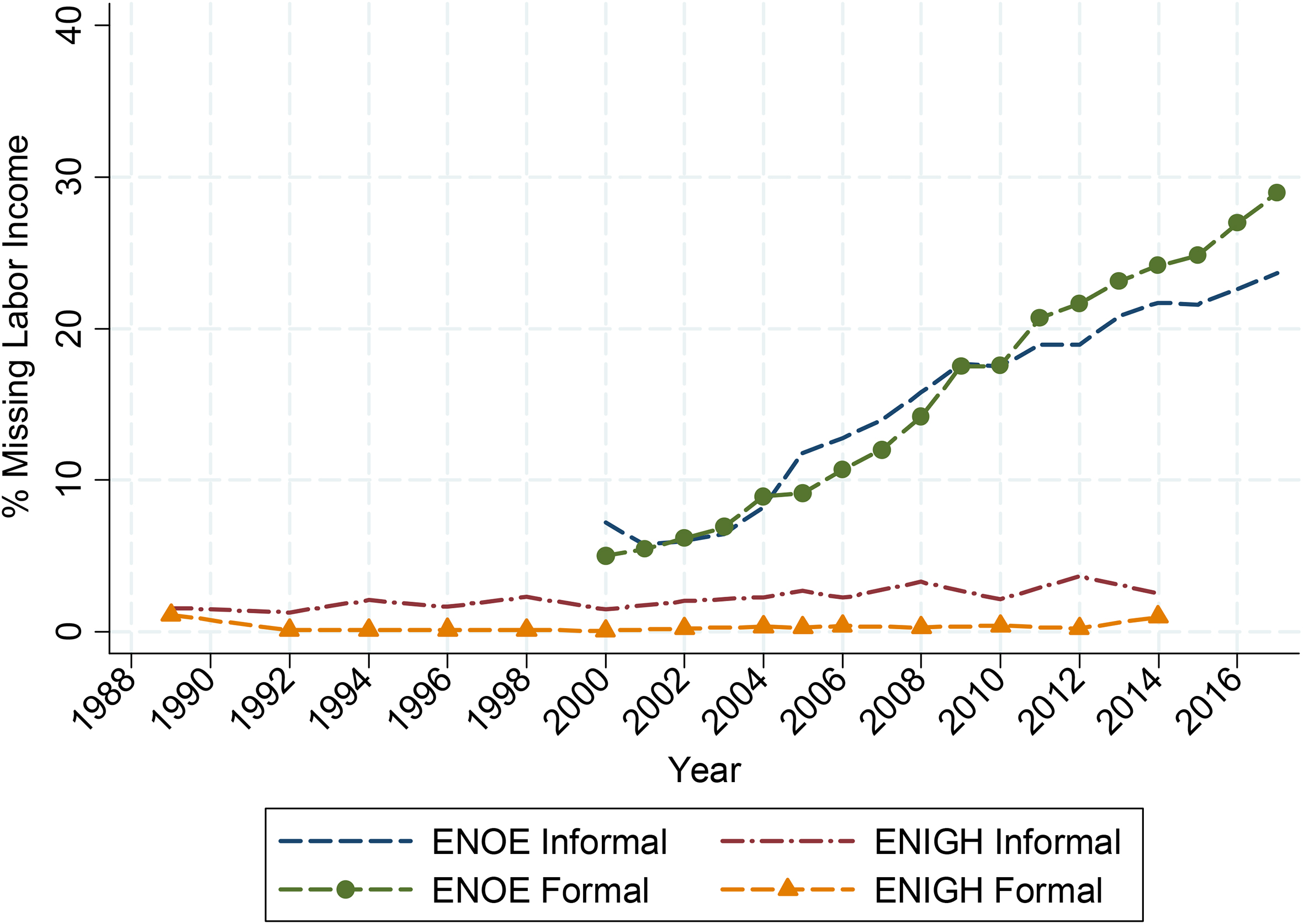

Although ENOE should be preferred to ENIGH given its sample size, it suffers from an egregious drawback: item non-response for labour income is higher and, worse, it has been increasing over time (Fig. 2).8 In 2017, item non-response reached a whopping 30 percent of all workers in ENOE. Why there has been such an increase in non-response for labour income in ENOE (but not in ENIGH) is a puzzle that remains unsolved.

In addition to item non-response, there is evidence that the surveys may suffer from undercoverage, especially, of high-wage earners. This can be easily confirmed in the case of formal workers. As shown in Table 1, IMSS data include a larger proportion of workers with two minimum wages and at the top of the distribution – those who earn more than ten and twenty times the minimum wage – than ENOE or ENIGH. Of relevance to our purposes, the under-representation of workers at the top increased over time, especially for ENOE. In 2000, the frequency of workers earning more than 10 MW equalled 3.8 percent in ENOE and 6.5 percent in IMSS. By 2017, the share was 2.1 percent in ENOE and 8.9 percent in IMSS. Workers earning more than 20 MW were 0.7 percent (ENOE) and 1.7 percent (IMSS) in 2000, while they were 0.2 percent (ENOE) and 2.7 percent (IMSS) in 2017.9 The extent of under-representation is lower in ENIGH but still substantial for workers earning at least ten times the minimum wage.

Table 1

Frequency of formal sector workers by multiple of the minimum wage in: 2000, 2010, and 2017/2014 (ENOE, ENIGH and IMSS, in %; total formal workers $=$ 100%)

	Multiples MW	ENOE	ENIGH	IMSS
2000	1–5	83.2	80.3	81.2
	6–10	13.0	14.5	12.4
	11–20	3.1	3.4	4.8
	21+	0.7	1.7	1.7
2010	1–5	81.6	77.3	75.3
	6–10	14.4	17.0	15.8
	11–20	3.5	4.6	6.4
	21+	0.6	1.1	2.5
2017/2014*	1–5	88.8	80.2	75.4
	6–10	9.1	14.9	15.7
	11–20	1.8	3.7	6.2
	21+	0.14	1.2	2.7

${}^{*}$ ENIGH data are for 2014. Notes: Sample restricted to formal sector workers aged 20–64 years with positive labour income and working hours. For ENOE we use the second quarter of each year. For IMSS data we report the value for the month of April of each indicated year except for 2000 and 2001, when we report the value for the month of December. Source: Authors’ construction.

Figure 3.

Frequency of formal sector workers by multiple of the minimum wage in: 2000, 2005, 2010, and 2017/2014 (ENOE, ENIGH, and IMSS, in %; total formal workers 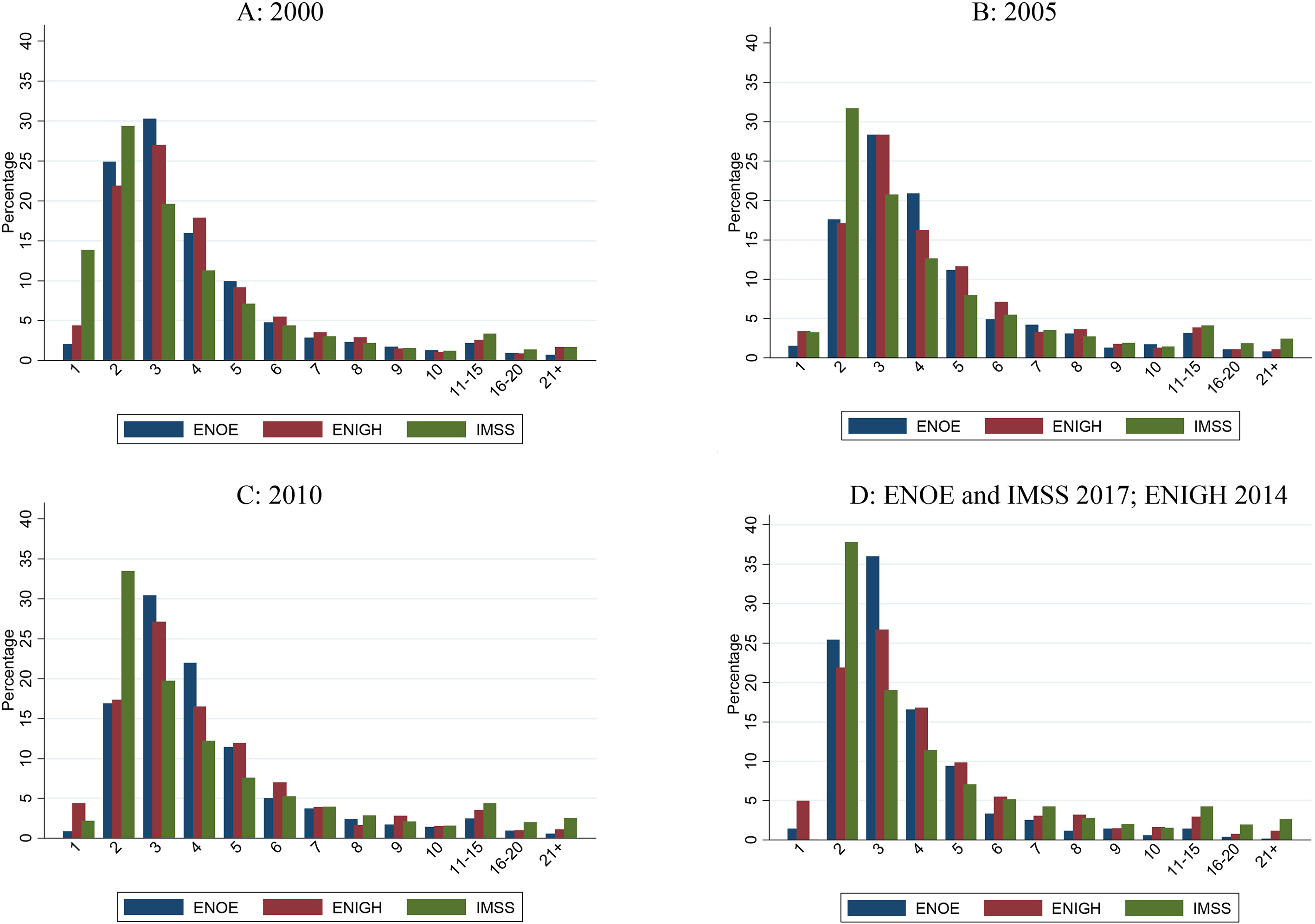$=$ 100%). Notes: Sample restricted to formal sector workers aged 20–64 years with positive labour income and working hours. For ENOE we use the second quarter of each year. For IMSS data we report the value for the month of April of each indicated year except for 2000, when we report the value for the month of December. Panel D for ENIGH refers to year 2014 because it was the most recent available at the time the analysis was completed. Source: Authors’ construction.

Some authors have attempted to correct for item non-response and under-reporting (which is also present in ENIGH) by adjusting (mainly, scaling up) the survey-based information to match totals in national accounts [15, 16]. Taking advantage of the fact that in 2016 the Mexican Institute of Social Security (IMSS) released (monthly) disaggregated data for formal sector workers by age, sex, and multiples of the minimum wage from 2000, here we follow a statistically more robust approach to correct for undercoverage in the upper tail of the labor income distribution for formal workers.10 In essence, we make a post-survey weight adjustment (i.e. change the expansion factors) in ENOE so that the frequency of individuals for categories of formal workers defined by age, sex, and multiples of the minimum wage in the surveys equals the frequency distribution observed in tabulations from the IMSS.11 In other words, we correct the distribution of labour income for formal sector workers on the assumption that the distribution of labour income in the IMSS data is the true distribution. We describe the method in more detail below. The theory behind this post-survey weight adjustment has a long tradition in statistics. For details see, for example [4].

2.2 Correcting for rising item non-response and undercoverage in the upper tail: ‘Hot deck’ imputation and post-survey reweighting

To correct for rising item non-response, we apply a typical ‘hot deck’ imputation method as proposed by [2]. This method is applied as follows. First, we define several sociodemographic groups (gender, age, schooling, state of residence). These groups contain workers with valid and missing income. Second, within those groups the income of a randomly selected sample is selected. Third, we substitute the missing income with observed income from other individuals within that group randomly.

As mentioned above, IMSS data include information on the number of workers in the formal sector by multiples of the minimum wage since 2000, and it also reports the brackets by gender and age group. Thus, it is possible to compare the distribution of formal workers by multiples of the minimum wage between IMSS and both ENIGH and ENOE (in the latter two datasets, we include the units with response on labour income only). Figure 3 and Table 1 show such a comparison for the years 2000, 2005, 2010, and 2017 (2014 in the case of ENIGH).

To correct for rising undercoverage of high-wage earners, we assume that the distribution of labour income of formal workers in the IMSS data is the true distribution and we reweigh individuals in ENOE so that the distribution of workers in the formal sector replicates the distribution of workers observed in the IMSS data. The new weights are calculated as follows. We classify workers in IMSS into categories by sex, age group (20–29, 30–39, 40–49, 50+), and multiples of the minimum wage (in groups: 1–10, 11–15, 16–20, 21+),12 or 104 (2 $\times$ 4 $\times$ 13) categories. We obtain the percentage of workers in the formal sector within each category and then replace these weights in ENOE so that the surveys end up with the same distribution of workers by category as in the administrative data. In other words, for each of the categories, we multiply the original expansion factors by the ratio

$\displaystyle\frac{\textit{\% Formal Workers in category in in IMSS}}{\textit{% \% Formal Workers in category in in survey}}$

Figure 4.

Frequency of formal sector workers by multiple of the minimum wage: 2005 and 2017 (ENOE and IMSS: original, and imputation and reweighting combined; in %; total formal workers 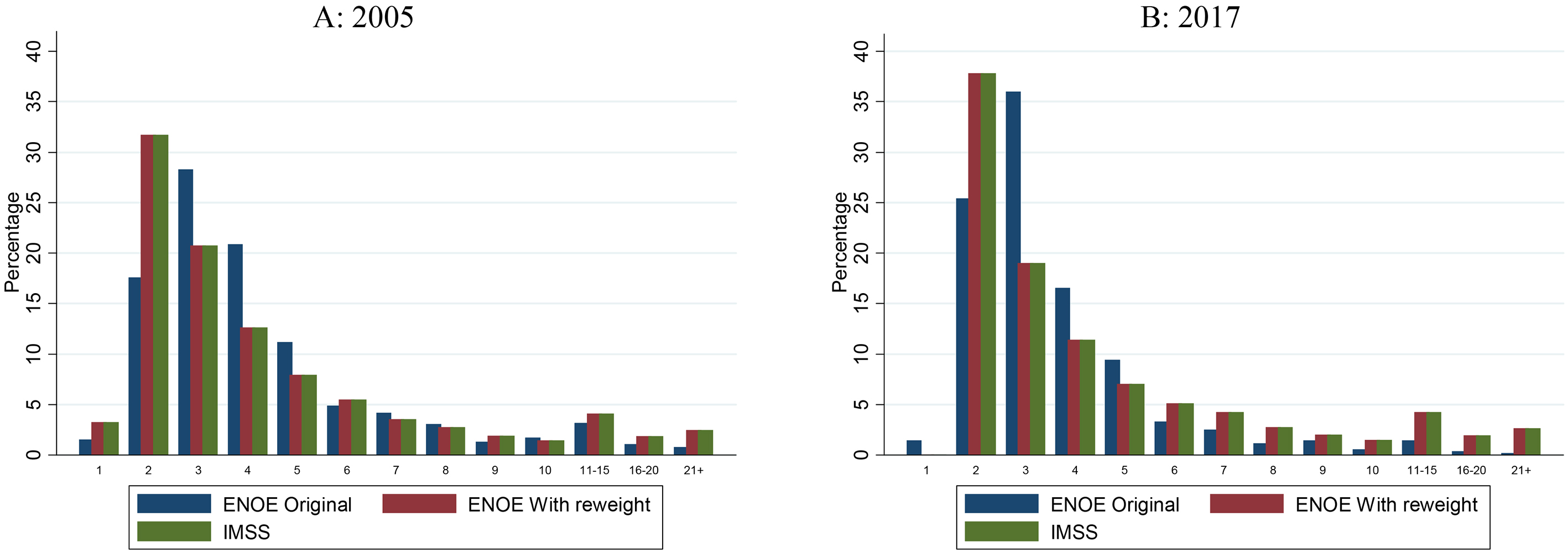$=$ A 100%). Notes: Sample restricted to formal sector workers aged 20–64 years with positive labour income and working hours. For ENOE we use the second quarter of each year. For IMSS data we report the value for the month of April of each indicated year except for 2000 and 2001, when we report the value for the month of December. For reweighting we use IMSS data. Source: Authors’ construction.

Figure 4 shows this reweighting process graphically for ENOE. Although due to data availability this correction method can be applied only from 2000 onwards, it is reassuring to note that the rise in item non-response in ENOE starts in the mid-2000s (Fig. 2), which is correlated with undercoverage of income by high income earners.

The post-survey reweighting method can only be applied to formal sector workers. While undercoverage could affect the sample of informal workers as well, there is no external information to implement a correction so for this group we use the base weights unchanged. In this paper, we refer to the post-survey reweighted data as ‘reweighted’ and the data with post-survey hot deck imputations as ‘imputed’. The data that include both corrections are called ‘corrected’. Given that all methods have their limitations, we carried out a series of robustness checks, which are discussed below.

2.3 Comparing original with reweighted and imputed data

Figure 5 shows average monthly labour income from the original and reweighted surveys (for formal workers) and imputed wages (for informal workers) for ENIGH and ENOE. We show the latter trends to point out that imputation only does not recover the trend shown in IMSS data. For formal workers, both the original and reweighted averages show a similar trend. The main differences are: (i) the decline between 2007 and 2010 (the so-called Great Recession) is smaller when using the reweighted measure and (ii) there is an increase in average labour income since 2015 with the reweighted measure but not with the original. Unsurprisingly given the reweighting method, the pattern of the reweighted surveys is similar to that observed with IMSS data, as shown in Fig. 6. Moreover, ENIGH original and reweighted are similar. This suggests that undercoverage of high earners is not a substantial problem in this survey and, thus, in the rest of the paper we only report results based on the ENIGH original data.

Figure 5.

Average monthly labour income for formal and informal workers: 2000–2017 (ENOE, ENIGH, IMSS: original and reweighted surveys; in constant Mexican pesos of August 2015). Notes: Sample restricted to workers aged 20–64 years with positive labour income and working hours. For ENOE we use the second quarter of each year. For reweighting we use IMSS data. Wage adjustment in the informal sector follows a hot deck imputation procedure using gender, region, informal status, age, and education group. Source: Authors’ construction.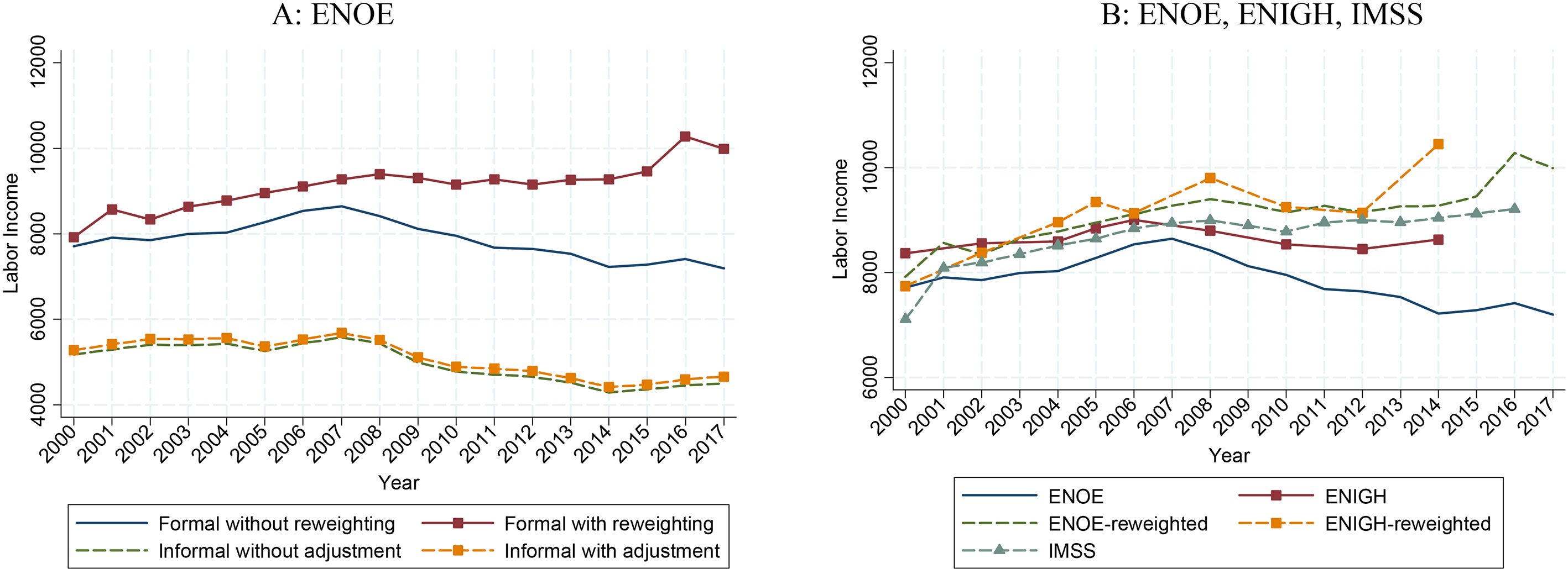

Figure 6.

Average monthly labour income for all workers: 2000–2017 (ENOE: original and corrected surveys; in constant Mexican pesos of August 2015). Notes: Sample restricted to workers aged 20–64 years with positive labour income and working hours. For ENOE we use the second quarter of each year. To correct for item non-response in ENOE, we follow a hot deck imputation procedure using gender, region, informal status, age, and education group. For post-survey reweighting for formal sector workers in ENOE we use IMSS data. Source: Authors’ construction.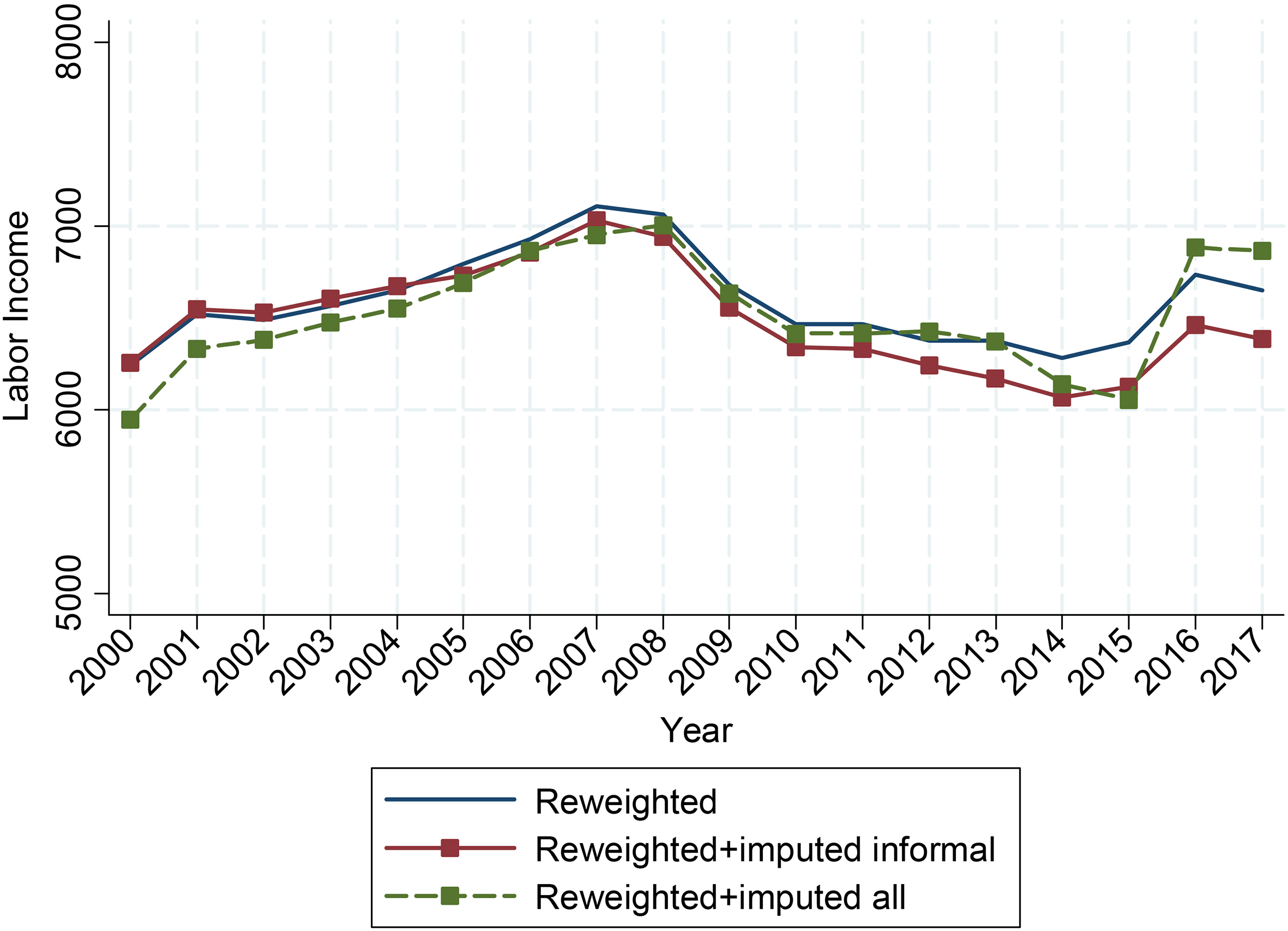

Figure 7.

Average monthly labour income for all workers by education: 1989–2017 (ENOE: original, reweighted, and imputed surveys; ENIGH: original surveys; in constant Mexican pesos of August 2015). Notes: Sample restricted to all workers aged 20–64 years with positive labour income and working hours. For ENOE we use the second quarter of each year. For reweighting we use IMSS data. Source: Authors’ construction.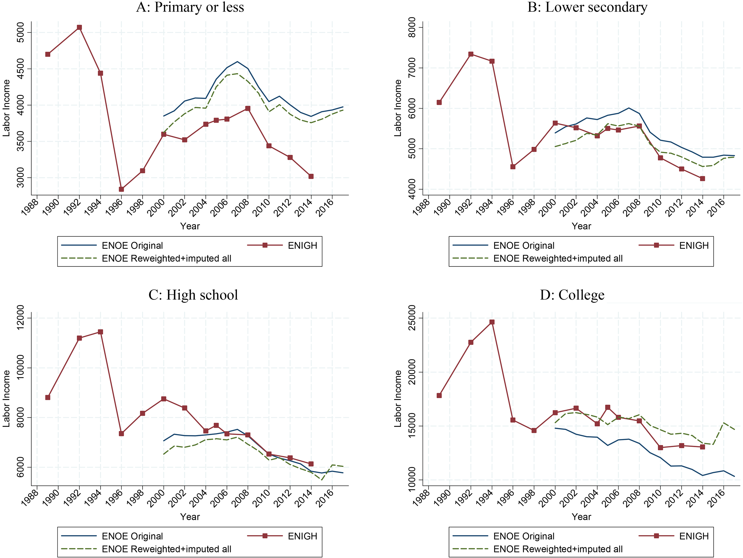

In Fig. 7, we show average monthly labour income for the original, reweighted, and imputed surveys by education. The first thing to notice is that the reweighting procedure mainly affects the trend for formal workers with a college education: while the original data show a steady decline, the reweighted surveys show that average labour incomes have remained largely unchanged since 2008 with an upswing after 2015. Since the reweighting method increases primarily the percentage of formal workers earning between one and two minimum wages and of those earning more than ten minimum wages, the reweighted averages tend to be slightly lower for those with less than a college education and higher for those with a college education. Moreover, in recent years the gap between the original average labour income and the reweighted measures has increased, especially in ENOE since 2008. When survey data have been reweighted (for formal workers) and imputed (for informal workers), the patterns are almost identical to those observed with reweighted-only surveys.

2.4 Robustness checks

In order to check the robustness of the correction methods followed here, we reweighted the surveys on the assumption that the true distribution in IMSS starts with the group earning five times the minimum wage or more and that below this threshold the data in the surveys are accurate. This correction yields almost exactly the same outcomes as those observed above. We also tried the rescaling method which has been applied by others [17]. That is, we did not change the weights but we replaced the average labour income for formal workers by centile in ENOE with the corresponding one in IMSS. Since the latter requires the entire population in IMSS and not just tabulations by multiples of the minimum wage, we were able to do this only for 2010 and 2012, the two years that these data were made available to our team.13 As we shall discuss further below, the most important difference with rescaled surveys versus reweighted surveys is that, using ENOE, from 2008 onwards the Gini coefficient rises instead of remaining roughly constant. In other words, with rescaled labour incomes, the trend in inequality is in even more stark contrast to the one observed with the original survey, which shows a steady decline. Finally, we also checked what might happen if we corrected the IMSS data for the fact that they are censored at the top using a Pareto approximation. While this correction increases the level of inequality, trends remain largely the same.

3. Labour income inequality: 2006–2017

As shown in Fig. 1, from 2006 onwards the Gini coefficient for labour income steadily declined with the original (uncorrected) ENOE survey but rose slightly with ENIGH. Thus, the two sources lead to almost opposite narratives as to the evolution of labour income inequality in this period. As shown in Fig. 2, however, there has been a sharp rise in item non-response in ENOE since 2006 for both formal and informal workers (roughly a third of workers in 2017). In Section 2 we explained how the ENOE data were corrected through a combination of the hot deck imputation method to ‘assign’ an income to non-respondents and a post-survey weight adjustment using IMSS tabulations for formal workers. Although ENIGH’s item non-response is lower and constant, we also produced results correcting with the same methods, which are available upon request.

Figure 8.

Labour income inequality: 1989–2017 (Original ENIGH and ENOE and corrected ENOE surveys). Notes: Sample restricted to all workers aged 20–64 years with positive labour income and working hours. For ENOE we use the second quarter of each year. Smoothed lines with a simple moving average with weights 0.4 for the current observation and 0.3 for the lead and lag. For post-survey reweighting for formal sector workers in ENOE we use IMSS data. To correct for item non-response for informal workers in ENOE, we follow a hot deck imputation procedure using gender, regions, informal status, age, and education groups. Source: Authors’ construction.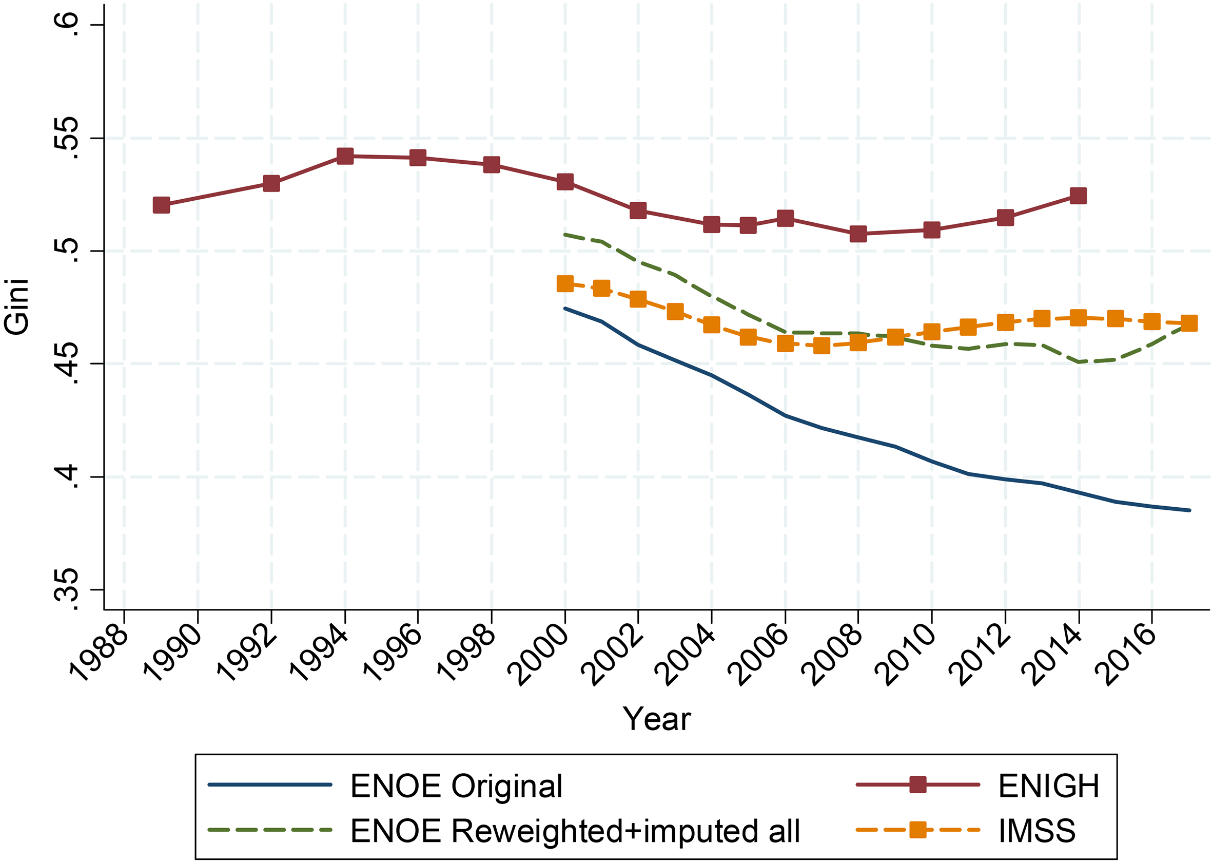

The effect of the correction on labour income inequality trends is notable. In Fig. 8 and Table 2, it can be observed that labour income inequality is higher for the corrected ENOE survey. In 2017, the Gini coefficient with the original ENOE survey equals 0.382, while it equals 0.464 with corrected data. An unsolved puzzle is that even for the corrected survey, ENOE shows much lower inequality than ENIGH. In 2014, ENIGH’s Gini coefficient for labour income for all workers equals 0.523, while it is 0.451 with ENOE corrected (Table 2).

Table 2

Gini coefficient for labour income for all workers: 1989–2017 (ENIGH, ENOE (original and corrected) and IMSS)

	ENIGH original	Original	Imputed all $+$ Reweighted (formal only)	IMSS (from tabulations for formal workers only)
		ENOE
1989	0.500 (0.013)
1992	0.541 (0.013)
1994	0.545 (0.008)
1996	0.539 (0.012)
1998	0.541 (0.006)
2000	0.534 (0.009)	0.476 (0.003)	0.513 (0.004)	0.489 (0.0004)
2001		0.473 (0.002)	0.501 (0.003)	0.482 (0.0004)
2002	0.516 (0.006)	0.456 (0.002)	0.498 (0.003)	0.480 (0.0004)
2003		0.447 (0.002)	0.485 (0.003)	0.474 (0.0003)
2004	0.504 (0.004)	0.452 (0.002)	0.485 (0.003)	0.467 (0.0003)
2005	0.517 (0.009)	0.433 (0.003)	0.467 (0.003)	0.461 (0.0003)
2006	0.511 (0.005)	0.424 (0.002)	0.464 (0.003)	0.458 (0.0003)
2007		0.424 (0.002)	0.461 (0.003)	0.458 (0.0003)
2008	0.516 (0.006)	0.416 (0.003)	0.466 (0.004)	0.458 (0.0003)
2009		0.413 (0.002)	0.461 (0.004)	0.462 (0.0003)
2010	0.491 (0.004)	0.410 (0.002)	0.458 (0.004)	0.465 (0.0003)
2011		0.395 (0.002)	0.454 (0.005)	0.466 (0.0003)
2012	0.526 (0.008)	0.400 (0.002)	0.458 (0.004)	0.469 (0.0003)
2013		0.402 (0.002)	0.464 (0.005)	0.471 (0.0003)
2014	0.523 (0.009)	0.388 (0.002)	0.451 (0.004)	0.470 (0.0003)
2015		0.390 (0.002)	0.438 (0.005)	0.470 (0.0003)
2016		0.388 (0.003)	0.471 (0.010)	0.470 (0.0003)
2017		0.382 (0.003)	0.464 (0.006)	0.466 (0.0003)

Notes: Sample restricted to workers aged 20–64 years with positive labour income and working hours. For ENOE we use the second quarter of each year. For IMSS data we report the value for the month of April of each indicated year except for 2000 and 2001, when we report the value for the month of December, and 2017, when we report the value for June. IMSS data are censored at twenty-five minimum wages or more. For post-survey reweighting for formal sector workers in ENOE we use IMSS data. To correct for item non-response for informal workers in ENOE, we follow a hot deck imputation procedure using gender, regions, informal status, age, and education groups. Standard errors in parenthesis are obtained using a bootstrap sampling procedure (250 replications) using the command ineqerr in Stata. Source: Authors’ construction.

For our purposes, an important result to note is the effect of the correction on labour income inequality. The corrected ENOE data no longer show the sharp fall observed in Fig. 1 between 2006 and 2017 (Table 2). Between 2006 and 2014, ENIGH shows an increase of about 1 Gini point and, with the corrected survey, ENOE stays the same. (If one were to apply the same correction method to ENIGH, however, the increase in labour income inequality during this period would be of 4 Gini points and the difference between the two sources would reach roughly 10 Gini points!) In sum, the evolution of inequality in the period after 2006 remains a puzzle unsolved. The most one can say with certainty is that labour income inequality definitely did not continue to decline.14,15

4. Conclusions

In this paper, we analyse the evolution of labour income inequality and its determinants in Mexico between 1989 and 2017. For the period prior to 2006, we identify two periods: 1989–1994, when inequality increased, and 1994–2006, when inequality declined. We review existing research on the role played by the skill premium (returns to education, in particular) in explaining these trends, and the extent to which trade patterns and technology affected relative returns.

For the period 1989–1994, there is a consensus that trade benefited high-skilled workers. The key channel through which trade affected wages was the establishment of maquiladoras and the decline or elimination of tariffs in low-skill-intensive industries. This combined with the erosion of institutional forces, including a declining rate of unionization and a falling real minimum wage. During this period, although the share of workers with college education increased, it did so at a slower pace than in subsequent periods. After NAFTA came into effect, inequality declined up to 2006.16 In contrast with the earlier period, the skill premium fell. Since institutional factors such as the minimum wage and the unionization rate remained constant during the entire period, the fall in the skill premium was associated with the fact that the supply of skilled workers outpaced demand.

After 2006, however, the measurement of labour inequality by itself becomes a challenge because the household income expenditure survey (ENIGH) shows a slight increase (Gini increases from 0.511 in 2006 to 0.523 in 2014) while the labour force survey (ENOE, without any corrections) shows a steady and sharp decline (from 0.424 to 0.388, in the same period). There is reason to believe that ENOE’s results are not accurate because the survey has not only a higher but also an increasing rate of item non-response (i.e. workers who do not report earnings). The proportion of workers who do not report their labour income reaches about a third of surveyed workers in 2017. We attempt to correct this problem by using a combination of the hot deck imputation method for all workers to get rid of non-response and a post-survey weight adjustment for formal sector workers. The post-survey reweighting uses recently released tabulations by the Mexican social security administration, IMSS. The new weights are such that the distribution of workers by categories of age, gender, and multiples of the minimum wage are the same in IMSS and ENOE.

The corrected ENOE no longer shows a steady decline in inequality: the Gini coefficient in both 2006 and 2017 is equal to 0.464. Thus, the most one can say is that after 2006 inequality stopped its downward trend. An unsolved puzzle is that even for the corrected survey, ENOE shows much lower inequality than ENIGH. In 2014, ENIGH’s Gini coefficient for labour income for all workers equals 0.523, while it is 0.451 with corrected ENOE. If we were to compare corrected ENOE with an equally (same methods) corrected ENIGH, the difference would be around a whopping 10 Gini points owing to the inclusion of the self-employed.

Footnotes

To place Mexico’s economy in context, the list of upper-middle income countries includes – among others: Brazil, China, Russia, South Africa and Turkey.

The theory behind this post-survey weight adjustment has a long tradition in statistics. For details see, for example [].

This result was found in many other studies. For example [6, 7, 8, 9, 10, ].

While there is a consensus in that demand for skilled workers slowed down, it has not been established which exactly were the causes of this slow down. One of the explanations considers that, possibly, technological change during this period was skilled labor-saving due to the introduction of digital technologies. Another explanation has to do with a rise in the relative cost of labor in the formal sector due to an increase in payroll taxes in conjunction with an increase in the subsidies for nonformal employment as a consequence of the expansion of noncontributory programs.

The labour force survey was first implemented in 1987 for a sample of cities and was called the National Survey of Urban Employment (ENEU in its Spanish acronym). The number of cities gradually increased. Between 2000 and 2004, the labour force survey was called the National Employment Survey (ENE) and thereafter it became the National Survey of Occupation and Employment (ENOE). For simplicity, we use the last acronym throughout to refer to the labour force survey.

For example, starting in 2008, the question regarding the aguinaldo (annual bonus) generated a figure for bonus income for the whole of the previous year, while before 2008 individuals were asked to give the amount of any bonus received the previous month. To avoid comparability issues, we removed the variable ‘Bonus’ from labour income in ENIGH. ENOE does not report bonus income, which also helps cross-survey comparability.

Formality here is defined by whether the worker contributes to social security.

The sample size for ENIGH is 19,419 households in 2014 (the last year we use here), much smaller than the labour force survey, which includes 107,274 households in 2014.

As the IMSS data are censored at twenty-five or more multiples of the minimum wage, the difference is in reality even greater.

IMSS data can be downloaded from http://datos.imss.gob.mx/.

Formal workers also include workers that are employed in the public sector. Although information on them is not included in the IMSS data, here we include these workers in the formal sector categories.

The IMSS data are censored at twenty-five or more multiples of the minimum wage.

We thank Facundo Alvaredo from the Paris School of Economics for sharing the rescaling factors for the total population for 2010 and 2012.

We calculated inequality using all workers and only salaried workers and found that the difference stems primarily from the self-employed because the inequality levels for salaried workers are much more similar.

We estimated a RIF regression (as in []) for the ENOE corrected survey and ENIGH original survey (supplementary materials). With ENOE corrected, the effect of characteristics continues to be unequalizing, as in the previous two periods. The returns effect continues to be equalizing but is no longer monotonical; it now mimics what happened along the income distribution. With ENIGH, the characteristics effect is no longer unequalizing but flat. The difference in results depending on the source is another puzzle that remains unsolved. Until the evolution of labour incomes along the distribution can be better assessed, this puzzle will remain.

NAFTA was signed between Canada, Mexico, and the United States at the end of 1993 and it came into effect on 1 January 1994.

Acknowledgments

This study has been prepared within the United Nations University World Institute for Development Economics Research (UNU-WIDER) project on ‘Inequality in the Giants’. We thank Luis F. López-Calva for his invaluable comments and suggestions and Alma Santillan for her excellent research assistance throughout the preparation of this paper. Earlier versions have been presented in seminars at UNAM (Mexico), the Paris School of Economics, LACEA conference and at the IEA World Congress at CIDE, Mexico. Comments and suggestions by Facundo Alvaredo, François Bourguignon, Carlos Ibarra, Jaime Ros, Emmanuel Saez, and other participants are gratefully acknowledged. We would like to thank the editor and reviewers for their thoughtful comments and efforts towards improving our paper. All remaining errors and omissions are the sole responsibility of the authors.

References

Campos-Vazquez

Lopez-Calva

Lustig

. Declining Wages for College-Educated Workers in Mexico: Are Younger or Older Cohorts Hurt the Most? World Econ. 2016; 43: 93-112. Available from https//www.sem-wes.org/es/node/1372.

Esquivel

Lustig

Scott

. Mexico: A Decade of Falling Inequality: Market Forces or State Action? In: Lopez-Calva

Lustig

, editors. Declining Inequality in Latin America: A Decade of Progress? Washington, DC and United Nations Development Programme (UNDP), New York: Brookings Institution Press, 2010, pp. 175-217.

Campos-Vazquez

. Why did wage inequality decrease in Mexico after NAFTA? Econ Mex. 2013; 22(2): 245-278. Available from http//www.economiamexicana.cide.edu/num_anteriores/XXII-2/01-EM_Campos_Vazquez.pdf.

Biemer

Christ

. Weighting Survey Data. In: Desirée de Leeuw

Hox

Dillman

, editors. International Handbook of Survey Methodology. New York: Psychology Press, Taylor and Francis Group; 2008, pp. 317-41. Available from: 10.4324/9780203843123.

Little

Rubin

. Statistical Analysis with Missing Data. Second Edition. New Jersey: John Wiley & Sons, 2002, p. 397.

Bouillon

Legovini

Lustig

. Can Education Explain Changes in Income Inequality in Mexico. In: Bourguignon

Ferreira

Lustig

, editors. The Microeconomics of Income Distribution Dynamics New York: The World Bank/Oxford University, 2005, p. 275-312. Available from: https//pdfs.semanticscholar.org/a199/d05219c7c17c6d64535688b148c937804d88.pdf.

Lopez-Acevedo

. Mexico: Evolution of Earnings Inequality and Rates of Returns to Education (1988–2002). Estud Econ. 2004 Jul; 19(2): 211-84. Available from: https//estudioseconomicos.colmex.mx/archivo/EstudiosEconomicos2004/211-284.pdf.

Lopez-Acevedo

. Mexico: Two Decades of the Evolution of Education and Inequality. In: Holsinger

James

, editors. Inequality in Education. Dordrecht: Springer. 2008, pp. 417-43. Available from: 10.1007/978-90-481-2652-1_18.

Meza-Gonzalez

. Cambios en la Estructura Salarial de México en el Período 1988-1993 y el Aumento en el Rendimiento de la Educación Superior. Trimest. Econ. 1999; 66(262): 189-26. Available from: https//www-jstor-org.web.bisu.edu.cn/stable/20856985.

10.

Popli

. Changes in Human Capital and Wage Inequality in Mexico. Oxford Development Studies. 2011 Sep; 39(3): 369-87. Available from: 10.1080/13600818.2011.596276.

11.

Campos-Vazquez

Esquivel

Lustig

. The Rise and Fall of Income Inequality in Mexico, 1989–2010. In: Cornia

, editor. Falling Inequality in Latin America: Policy Changes and Lessons. New York: Oxford University Press, 2014, Available from: https//www.oxfordscholarship.com/view/10.1093/acprof:oso/9780198701804.001.0001/acprof-9780198701804.

12.

Firpo

Fortin

Lemieux

. Unconditional Quantile Regressions. Econometrica 2009 May; 77(3): 953-73. Available from: 10.3982/ECTA6822.

13.

Bound

Johnson

. Changes in the Structure of Wages in the 1980s: An Evaluation of Alternative Explanations. Am Econ Rev. 1992 Jun; 82(3): 371-92. Available from: https//www-jstor-org.web.bisu.edu.cn/stable/2117311.

14.

Bourguignon

Ferreira

Lustig

. The Microeconomics of Income Distribution Dynamics in East Asia and Latin America. Washington, DC: Oxford University Press, 2008, 416.

15.

Campos-Vazquez

Chávez

Esquivel

. Estimating Top Income Shares Without Tax Return Data: Mexico Since the 1990s. Latin American Policy. 2018; 9(1): 139-63. Available from: 10.1111/lamp.12143.

16.

Del Castillo

. La magnitud de la desigualdad en el ingreso y la riqueza en México: una propuesta de cálculo. Ciudad de México: CEPAL, 2005, 249p. Available from: https//repositorio.cepal.org/bitstream/handle/11362/39531/1/S1501288_es.pdf.

17.

Piketty

Yang

Zucman

. Capital Accumulation, Private Property and Rising Inequality in China 1978–2015. Am Econ Rev. 2019 Jul; 109(7): 2469-96. Available from: 10.1257/aer.20170973.