Top expenditure distribution in Arab countries and the inequality puzzle 1

Abstract

This study was motivated by reports of a mismatch between inequality experienced on the streets across the Arab region, and that estimated in household expenditure surveys. The study uses eleven surveys from Egypt, Jordan, Palestine, Sudan and Tunisia to investigate whether the dispersion of top expenditures and measurement errors in them bias the measurement of inequality. The expenditure distributions are corrected by replacing potentially mismeasured values with those drawn from parametric distributions. Across all surveys, expenditure inequality is found to be at or below that found in emerging countries worldwide. The Gini is consistently 0.30–0.32 in Egypt, 0.35–0.37 in Jordan, and 0.38–0.43 in Palestine, Sudan and Tunisia. Several surveys include outliers raising inequality estimates. The Egyptian, Palestinian, and Tunisian surveys exhibit smoother top tails of expenditures, approximable by parametric distributions. Across years leading up to the Arab Spring, the estimates in these countries show falling inequality, suggesting that data problems are not behind the Arab inequality puzzle.

Keywords

Top expenditures economic inequality Pareto law Arab region

1. Introduction

In 2011 a series of revolutions shook the Arab region bringing about political changes in a number of countries. Worldwide attention turned to explaining the causes of these revolutions, and their repercussions. The prevalent theory since the days of the revolutions has held that inequality played a central role in the stirring up of popular discontent. The extent to which different dimensions of inequality were responsible for regime change in Egypt, Libya, Tunisia and Yemen – and other significant political upheavals in Bahrain, Jordan, Morocco, and Syria – and the acuteness of the different dimensions of inequality in the first place, are the subject of an active academic discourse [2, 3, 4, 5, 6, 7, 8].

The true level, manifestation and trend of inequalities in the lead up to the Arab Spring are all points of contention. Perceptions on the street and by the region’s commentators are that inequality and lack of access to career opportunities are problems that played a crucial role in triggering the uprisings [9, 10]. Grievances held by the middle class against the privileged elites were also specifically cited as culprits [1]. This narrative is rooted in regional history. Public outcries about inequality, lack of freedoms and cronyism were not confined to the years leading up to the Arab Spring, but can be traced back at least three decades to movements against authoritarianism [12], austere neoliberal reforms [13, 14] and a “fusion between neoliberal and authoritarian forces” [15]. The protests against oppression can be traced even longer to the ‘Great’ revolutions of the first half the 20 ${}^{\text{th}}$ century freeing the region of the oppression under the old social structures including colonialism, monarchy and feudalism [16].2

However, the foregone conclusions about high inequality leading to the Arab Spring are in contrast to objective measurements of inequality using household surveys, a phenomenon dubbed the Arab inequality puzzle [17]. Bibi and Nabli [18] reviewed the available evidence of inequality in the region and concluded that Arab countries in particular fall within the range of countries with moderate inequality of household incomes and expenditures, when compared to other regions such as East Asia, Latin America, South Asia and Sub Saharan Africa. Inequality measures based on both the Gini coefficient and the aggregate share of the top to bottom deciles – often measured in terms of consumption expenditures – have been relatively low and declining.

The low inequality estimates in household surveys do not appear to be due to poor data quality. While there are presently few parametric tests of the properties of income, expenditure and wealth distributions in the region [19], several recent studies have re-estimated inequality using parametric methods robust to various measurement issues pertaining to data quality, survey representation and non-response.

A world-wide historic study using an assumption of lognormal income distributions anchored by national accounts statistics [20] concluded that over the prior decades the Arab region had seen progress in reducing poverty rates and converging toward the world average welfare level and contribution to a “global middle class”. More relevant to our analysis, several studies have analyzed the top ends of individual countries’ income distributions using external data on real estate postings [21], national accounts and tax microdata [22, 23], or parametric values from other mostly developed countries [24]. Using stylized parametric assumptions, or parameter values rather atypical of the region, they estimated higher degrees of national and cross-country inequality [25].

Alvaredo and Piketty [24] estimated inequality using a mix of Pareto distributions for top incomes and log-normal distributions for the rest of incomes. In Egypt as well as in the rest of the Arab region, this approach yielded higher estimates of inequality, suggesting systematic underreporting of top incomes, but the new national estimates were still moderate. On the other hand, between-country gaps in income distributions gave rise to high estimates of inequality at the pan-Arab level. Assouad [22], applying the same methodology as Alvaredo and Piketty to the individual tax returns and national accounts data in Lebanon, found one of the highest income concentrations among all the countries included in the World Top Income Database due to the disproportional effect of profits and rents in the top quantiles. Extrapolating these high estimates to the rest of the Arab region yielded high measures of national and particularly region-wide inequality.

Using within-survey information alone, Hlásny and Verme [26] found that replacing actual top incomes or expenditures in the Egyptian household survey with Pareto parametric estimates did not affect the computed Gini noticeably regardless of how data were weighted, apparently on account of the adequate quality of the data. Hlásny and Verme [27] evaluated the dispersion of top incomes in several countries worldwide by comparing the actual dispersion to that predicted under the Pareto or the four-parameter generalized beta type-II (GB2) distributions. They found that the use of the Pareto distributions resulted in larger corrections as compared to the use of GB2 distributions but the differences were modest. In Egypt, the observed top 0.1% of incomes were found to be extreme or overstated (commanding a downward correction). However, the following 1% of incomes were found to follow the expected distributions more closely.

Focusing on the opposite tail of income distributions across a large set of Mediterranean surveys, Hlásny et al. [28] assessed the presence and dispersion of non-positive incomes, and corrected the distribution using non-parametric and parametric methods. They found that negative and zero incomes are quite prevalent in the region, and are associated with self-employment earnings or with large tax or social-security adjustments. Households with non-positive incomes do not appear to be materially deprived, and their various socio-economic outcomes would predict much higher, positive income levels. Replacing non-positive incomes with the predicted positive incomes results in estimating an even lower degree of inequality.

This review suggests that income and consumption are prone to various measurement errors. The challenges are more severe still for households’ wealth, which is an important determinant of workers’ career outcomes [29]. Among the handful of existing studies, Hlásny and AlAzzawi [30] estimate the distribution of durable-asset wealth across three Arab countries and across up to three survey waves, taking into account an extensive list of productive and non-productive assets. They found that the distribution of asset ownership was closely associated with the distribution of households’ income and other socioeconomic outcomes. El Enbaby and Galal [31] assessed inequality of opportunity for wealth acquisition and for earnings in Egypt during 1998–2012, showed their distributions, and discussed the complementary relationship between them.

This study adds to the literature by evaluating the dispersion of top expenditure observations in five countries in the Arab region using several alternative modeling specifications, and testing whether the potential mismeasurement of top expenditures could be driving the Arab inequality puzzle. The first contribution is to describe the top of the expenditure distributions in several Arab countries, including the rarely studied Palestine and Sudan, and provide parametric measures of the degree of dispersion of top expenditures. The second contribution is to deal with the suspected top expenditure issues by replacing actual top observations with values predicted under the Pareto distribution of type I – theoretical distribution used commonly as a good approximation to true population distributions across countries and years [32, 33, 34, 35]. Going beyond the analysis by Hlásny and Verme [26, 28], several robustness tests are performed with respect to model specification.

By design, synthetic values drawn from the Pareto distribution are less prone to measurement errors, data censoring, or year-to-year sampling errors than empirical observations. They allow us to produce more accurate estimates of inequality, and changes in inequality across survey waves. By comparing the fit of the Pareto distributions to the actual patterns of dispersion of top expenditures, we can assess how adequately rich households are represented in Arab region surveys, and how sensitive the observed levels and trends in inequality are to measurement and sampling errors. Ultimately, the methods and findings in this study will serve to advance the toolbox for scholars and policymakers in the Arab region for working with regional economic distributions.

The paper is organized as follows. Section two briefly describes the data, empirical issues and correction methods taken up in the analysis. Section three presents the main results and section four discusses their significance with respect to the broader problem of evaluating economic inequality across the Arab region and over time.

2. Survey data, right-tail measurement issues, and correction methods

The central aim of this study is to advance our understanding of the distribution of welfare among the peoples of the Arab region, using recently developed estimation methods and a newly available set of high-quality, harmonized household surveys. Expenditure per capita is used as a welfare aggregate [36]. The reason for preferring expenditures over incomes is that the set of surveys used in this study are for emerging economies with significant rural sectors, where households earn incomes in kind, and engage in household production. The corresponding streams of consumption and welfare are better captured through questions about implicit consumption expenditures than about incomes.

The reliance on expenditures also facilitates comparison with other countries in the region as well as worldwide for whom income microdata are unavailable, are mismeasured or are not as yet analyzed carefully. Another reason for using expenditures is that expenditure data may be more precise given that income may be underreported, and given that expenditure is smoother than income over time, especially in developing and rural areas. Moreover, expenditure data in the Arab region have been found to exhibit lower inequality than incomes [18], potentially presenting an even greater puzzle to observers of the recent political developments and changes in the region. The relatively narrow distribution of top expenditures may be on account of high saving elasticity among the rich, or may potentially indicate measurement issues that are more serious than those in the case of top incomes (e.g., imputed rent, expenditures abroad, illicit goods and services).

2.1 Available data

Most Arab countries conduct household income and expenditure surveys (HHIES) periodically to collect evidence regarding the distribution and components of incomes and expenditures of their population. However, not all countries make the survey micro-data publically available in their entirety or at all. This study relies on a set of HHIESs harmonized and released to the public by Economic Research Forum (ERF) in collaboration with national statistical agencies: the Egyptian Household Expenditure, Income and Consumption Survey; the Jordanian Household Expenditure and Income Survey; the Palestinian Expenditure and Consumption Survey; the Sudanese National Baseline Household Survey; and the Tunisian National Survey on Household Budget, Consumption and Standard of Living. These are high quality, well-documented surveys that have been validated and used successfully in a number of existing studies [8, 28, 37]. All HHIES surveys are nationally representative, and thus comparable across countries and years, but individual households cannot be tracked over time.

All recent HHIESs available at the time of writing are used, including the surveys for Egypt 2008, 2010 and 2012; Jordan 2006 and 2010; Palestine 2007, 2010 and 2011; Sudan 2009; and Tunisia 2005 and 2010. The Egyptian surveys were administered during April ‘08–March ‘09, July ‘10–June ‘11, and July ‘12–June ‘13, that is two years before the uprising, in its midst, and during the flux one year after the uprising when the Muslim Brotherhood was promoting a new national constitution. The Jordanian surveys were collected in the 12 months following April ‘06, and those following April ‘10 – for the most part before public protests in the country became widespread in the spring of 2011 and led to constitutional reforms. In Palestine, the surveys were collected throughout the years 2007, 2010 and 2011, at the time of relaxation of the Israeli security regime and prior to the September 2012 surge of major protests against domestic economic policy. In Sudan, the survey took place in the summer of 2009, three years prior to the start of Arab-Spring inspired protests against the government’s austerity plans. Finally, the Tunisian surveys were administered during May ‘05–May ‘06, and June ‘10–May ‘11. Fieldwork for the second survey was thus at its height in January 2011 when major public protests erupted, motivated by people’s economic and democratic concerns, and led to the toppling of the country’s president.

In the following analysis, the surveys are used one by one as cross-sectional samples. We are able to use multiple survey waves for four of the five included countries. This allows us to follow the evolution of expenditures and of inequality over time, and in the case of Egypt before and after the popular uprising. While the five countries do not represent the entire Arab region, they show a mosaic of the economic conditions and survey practices across the region. The surveys differ in their sampling rate from the population, and cover a heterogeneous block of countries in terms of their economic development, demography and labor force composition, inequality, and political climate at the time of survey fieldwork. Table 1 presents the essential information on survey sources and data distribution. Additional information is provided in the supplementary materials.

Table 1
Data sources and summary statistics

Country, year	Fieldwork	Survey	Households	Mean expenditures per capita (st.dev.) ${}^{\text{a}}$	Med. expend. per cap.
Egypt 2008	01.04.08–30.03.09	HEICS 2008/09 [59] ${}^{\text{bc}}$	23,428	1,425.38 (1,221.58)	1,151.06
Egypt 2010	01.07.10–30.06.11	HEICS 2010/11 [60]	7,719	1,603.37 (1,352.69)	1,287.40
Egypt 2012	01.07.12–30.06.13	HEICS 2012/13 [61]	7,525	1,719.77 (1,251.38)	1,414.53
Jordan, 2006	01.04.06–30.04.07	HEIS 2006 [62]	2,897	2,500.05 (2,274.26)	1,927.28
Jordan, 2010	01.04.10–30.04.11	HEIS 2010/11 [63]	2,845	3,108.79 (4,139.79)	2,348.79
Palestine 2007	15.01.07–14.01.08	PECS 2007 [64]	1,231	3,759.11 (3,756.81)	2,759.62
Palestine 2010	15.01.10–14.01.11	PECS 2010 [65]	3,537	5,138.56 (5,012.92)	3,771.70
Palestine 2011	15.01.11–14.01.12	PECS 2011 [66]	4,317	5,280.86 (4,878.28)	3,964.53
Sudan, 2009	17.05.09–30.06.09	NBHS 2009 [67]	7,913	1,164.74 (1,260.34)	881.01
Tunisia, 2005	05.05.05–04.05.06	EBCNV 2005 [68]	12,318	2,600.67 (2,818.96)	1,894.29
Tunisia, 2010	01.06.10–01.06.11	EBCNV 2010 [69]	11,281	3,332.21 (2,930.51)	2,542.90

${}^{\text{a}}$ Converted to year-2005 purchasing-power parity international dollars. For lack of availability of newest data, year-2007 conversion rate is used for all Palestinian surveys. Summary statistics account for household sampling weights and household size. ${}^{\text{b}}$ HEICS $=$ Household Expenditure, Income and Consumption Survey; HEIS $=$ Household Expenditure and Income Survey; PECS $=$ Palestinian Expenditure and Consumption Survey; NBHS $=$ National Baseline Household Survey; EBCNV $=$ National Survey on Household Budget, Consumption and Standard of Living. ${}^{\text{c}}$ ERF data are 30–50% random extractions from original HEICS surveys administered by Egyptian Central Agency for Public Mobilization and Statistics, which include 48,658 (HEICS 2008/2009), 26,500 (HEICS 2010/2011) and 24,863 households (HEICS 2012/2013).

Before any analysis with the available sample, it is useful to check whether extreme expenditure observations are simply errors such as data-entry errors or are true values incidentally very distant from the central moments of the expenditure distribution. The eleven surveys differ significantly in the level and the dispersion of the highest several expenditures. The Egyptian data exhibit modest dispersion. The single highest expenditure exceeds the one ranked twentieth by merely 190 percent in 2008, 210 percent in 2010, and 120 percent in 2012.3 The Jordanian data show more substantial dispersion, and include an influential observation in the 2010 wave. In the 2006 wave, the highest observed expenditure per capita exceeds the second highest one by 64 percent, and the twentieth highest one by 354 percent. In the 2010 wave, on the other hand, the highest expenditure per capita is more than seven times as high as the one in the second place, and more than twelve times as high as the one ranked twentieth.4

In Palestine 2010, similarly, the highest one or two expenditures appear extreme. In the 2007 and 2011 waves, the single highest expenditure is 29–43 percent higher than the second highest expenditure, and 189–262 percent higher than the one ranked twentieth. In 2010, however, an outlying top expenditure is 134 percent higher than the second highest one, and more than seven times as high as the twentieth highest one. It is likely that the small sample sizes in Jordan ‘10 and Palestine ‘10 are partially responsible for the presence of outliers.

In Sudan, the highest observed expenditure per capita exceeds the second highest one by 29 percent, and the twentieth by 189 percent, a medium degree of top expenditure gaps. In both waves of the Tunisian survey, the household with the highest expenditure per capita surpasses the expenditure of the second richest household by a mere 17–23 percent. Similarly, it surpasses the expenditure of the twentieth household by only 211–213 percent. Rather than having a single outlier, the Sudanese and Tunisian surveys have 3–4 outlying households – their expenditures are clustered nearby each other, while they exceed the following values by 50 percent. On the other hand, no further clustering of observations is found lower down the expenditure distribution.

Assessing the aggregate-expenditure shares of the richest households, we find that they are higher in Jordan, Palestine and Sudan and lower in Egypt and Tunisia (last row in Table A1). Since it is unclear whether the dispersion of top expenditures in one survey (Jordan, or Palestine) is too wide due to measurement issues, or the dispersion in another survey (Tunisia) is too narrow due to underreporting, we take an agnostic view of the validity of each observation, and let parametric estimation on the entire distribution of top expenditures tell us which observations step out of line relative to the predicted pattern.5

Table 2 provides additional information on the actual distribution of top expenditures: the share of aggregate expenditures accounted for by the top 0.1 percent of observations (or 7–11 households across surveys) to as many as 20 percent of observations (or 780–2,662 households) are shown in brackets. These results confirm a disproportionate concentration of wealth among the super-wealthy 0.2 percent of households (19–21 units) in Jordan ‘10 and in Sudan, where they command over 2.9–3.0 percent of aggregate expenditures. Tunisia ‘05 is nearly at that level of concentration among the uppermost expenditure households. Regarding expenditure shares among the following 20 percent of households, Sudan and Tunisia ‘05 exhibit disproportionate concentrations. The richest 1 percent (10%, or 20%) of households control 7.6–7.8 percent (30.8–32.4 or 46.3–48.0%, respectively) of aggregate expenditures.

2.2 Top income measurement issues

The observations in the uppermost tail of expenditure distributions may reflect true values of expenditures in the population, and may be appropriate to include for the sake of measuring inequality in the population. Alternatively, extreme observations may arise due to various errors and, if included, should be corrected for the identified errors. In either case, the uppermost observations may introduce spurious volatility of inequality across survey waves.

It is well known that the inclusion of extreme observations tends to influence commonly used measures of inequality [40]. Some measures such as the Theil index and other Generalized Entropy indices are very sensitive to exact values of top observations, but even the Gini coefficient is not robust to them [41]. To evaluate how sensitive inequality measurement is to extreme expenditure observations, without judgment on their authenticity, we would want to identify which observations are outliers and estimate our measures of inequality with and without them. Neri et al. [42], for example, define outliers in the EU Surveys on Income and Living Conditions (SILC) as observations exceeding the median 4–5 times, and find that this comprises 0.1–0.2% of households.

In HHIESs measurement errors may arise for several reasons, including intentional misreporting, errors in recollection, or data entry errors. Across survey waves, expenditure distributions may also exhibit different upper tails on account of sampling variability. Top expenditures may generally also be deliberately obscured by national statistical agencies to comply with privacy norms or correct for measurement problems, but this is not the case with the survey samples at hand. Due to the potential measurement problems and sampling differences across survey waves in our set of Arab household surveys, our estimation of inequality levels and trends may be biased. We thus turn to a recently promulgated correction method that can address these issues.

2.3 Replacement using values from a Pareto distribution

To compare the actual distributions of top expenditures to distributions that may be predicted in the given countries, and study the presence of extreme values in our data, we follow an approach applied by Atkinson, Cowell, Jenkins, Piketty and others to summarize the dispersion of economic outcomes by a parametric distribution, report properties of the estimated distribution, and use the estimates to correct the observed top tail for suspected statistical problems [38, 43].

Inequality estimates imputed from parametric distributions can be less sensitive to extreme observations and sampling variations than non-parametric observations from actual survey data. Parametric estimates for the top tail could be combined with non-parametric statistics for the rest of the distribution to obtain estimates with better empirical properties [32, 41]. Burkhauser et al. [44] compared four methods for dealing with under-representation or top-coding in the survey data – essentially replacing top-coded values using four alternative parametric estimators and combining the estimates with non-topcoded observations.

The following estimation approach is motivated by an empirical regularity that top observations across countries and years follow a particular pattern represented well by the Pareto distribution. Arnold [45] reviews the properties of the Pareto distribution as well as of the broader family of Pareto distributions. The Pareto distribution is highly skewed and heavy-tailed, and is thought to be suitable to model upper incomes, expenditures, wealth or other welfare aggregates [46, 47, 48]. As expenditures grow larger, the number of observations declines following a law dictated by a constant Pareto coefficient $\theta$ . The Pareto distribution can be described by its probability density function as follows:

$\displaystyle f(x)=\frac{\theta}{x^{\theta+1}},1\leqslant x\leqslant\infty.$ (1)

Here $x$ is the variable of interest, which in our case will be expenditure per capita in international purchasing-power parity dollars. The Pareto coefficient $\theta$ can be estimated by maximum likelihood methods [39, 49] as

$\displaystyle\theta=\frac{1}{{\log x_{(n-k+1)}}-k^{-1}\sum^{k-1}_{i=0}({\log x% _{(n-i)}})},$ (2)

where $x_{(j)}$ is the $j$ th order statistic in the sample of expenditures $n$ , and $k$ is the delineation of top expenditures such as the top 10% of observations [50].

2.4 Replacement using randomly drawn rather than predicted values

Replacing observed expenditures with fitted values from the Pareto distribution yields measures of expenditure distribution and inequality that do not account for parameter-estimation error and sampling error in the available dataset. This problem is on top of the issue of combining standard errors of the parametric Gini among top expenditures and the nonparametric Gini among lower expenditures. An and Little [51], and Jenkins et al. [52] account for sampling error by drawing random values from the estimated distribution for all potentially imprecise top observations, combining them with actual lower-level values, and calculating a quasi-nonparametric inequality measure (that is, inequality measure estimated non-parametrically on partially synthetic data) with its bootstrap standard error. Repeating the exercise multiple times, we can note variability in the obtained inequality measure. Following Reiter [53], the expected measure of inequality in such partially synthetic data can be computed as a simple mean of inequality measures from individual random draws, $\textit{Gini}_{\textit{quasi}}$ :

$\displaystyle\widehat{\textit{Gini}_{\textit{quasi}}}=\sum^{m}_{i=1}\textit{% Gini}_{\textit{quasi\ i}}/{m}$ (3)

Its sampling variance can be computed as:

$\displaystyle\widehat{\text{var}}=\frac{\sum^{m}_{i=1}\left(\textit{Gini}_{% \textit{quasi\ i}}-\widehat{\textit{Gini}_{\textit{quasi}}}\right)^{2}/(m-1)}{% m}+\sum^{m}_{i=1}\text{var}_{\textit{quasi\ i}}/{m}.$ (4)

The first term here is the sampling variance across different draws from the Pareto distribution, and the second term is the mean sampling variance within an individual draw. $m$ is the number of repetitions and $\text{var}_{\textit{quasi\ i}}$ is the variance of the quasi-nonparametric Gini coefficient from an individual draw $i$ . This methodology still ignores standard error from the estimation of parameters in the Pareto distribution. However, this is expected to be quite small compared to the sampling error, and can be ignored in large datasets where parameters have been estimated precisely [52].

The quasi-nonparametric Gini coefficient can be compared to an uncorrected nonparametric estimate. As long as it was correct to assume that top expenditures in the population are distributed as Pareto, a difference between the quasi non-parametric and non-parametric estimates would indicate that some observed high expenditures may have been generated by a statistical process other than Pareto, and that our inequality measure is sensitive to this. Quasi non-parametric Ginis that are lower than non-parametric Ginis can be interpreted as evidence that some top expenditures in the national samples are extreme compared to those generated under the Pareto distributions. A higher quasi non-parametric Gini would indicate that the observed top expenditures are lower than what would be generated under the Pareto distribution, potentially implying under-representation of rich units or underreporting of top expenditures in the sample.

In the following empirical analysis top expenditures are replaced by random draws from the Pareto distributions estimated on them. The reason for estimating the distributions on the same observations as those that will be replaced (rather than, say, estimating right-truncated Pareto distributions only on lower expenditure values deemed reliable) is that this approach allows us to remain agnostic regarding the validity of any individual observation. The approach does not require us to decide a priori which observations to use for estimation, and which observations to replace. Consequently, this approach can be viewed as addressing the problem when some expenditures are randomly under- or over-reported, or rank-proximity swapped. To the extent that different survey waves manage to cover different top-expenditure households through random sampling, this approach also mitigates the problem of overestimation of the variation in inequality across survey waves due to sampling errors. However, this approach cannot address problems of stand-alone systematic underreporting or top-coding of expenditures [54].

For the choice of an inequality index, this study uses the Gini coefficient as the primary measure, for its properties of being well understood and easily estimable under both parametric and nonparametric distributions, widely reported, and less sensitive to extreme observations than other indices. The results of inequality corrections in this study can thus be viewed as conservative estimates for the true effects of extreme observations on inequality measurement in general, under the baseline hypothesis that top-income issues do not affect inequality measurement in the Arab region. To the extent that the estimated Gini is affected by measurement issues, we may safely conclude that the consequences for other inequality measures would be as large or larger. For comparison, Table A4 reports the top expenditure shares in the actual and corrected distributions.

Finally worth noting, the statistical analyses undertaken in this study were implemented using algorithms [49, 55, 56] for Stata version 13, on an Intel Core i5 CPU laptop running at 2.50 GHz with 8 GB of memory, running Windows 10 64-bit Professional operating system.

3. Results

Table 2 presents quasi-nonparametric estimates of Gini coefficients, obtained by replacing top expenditure observations with random values drawn from smooth Pareto distributions estimated among these top observations. The first row in Table 2 shows the benchmark nonparametric estimates of the Gini for each survey. The following rows present the quasi-nonparametric estimates from the distributions of household expenditures per capita when the top 0.1–20.0 percent of values are replaced by numbers drawn randomly from the corresponding Pareto distributions.

Table 2 shows that the correction for potentially mismeasured top expenditures varies across the eleven surveys. In the three Egyptian surveys, the replacement of top 0.1–5 percent of expenditure observations leads to a small but systematic increase in the Gini of 0.3–0.4 percentage points. This suggests that the reported expenditure values are distributed slightly more narrowly compared to what one would expect following the Pareto law. Thus, we do not find evidence that the topmost 0.1% of expenditures are extreme or command a downward correction, as Hlásny and Verme [26] found for incomes in 2008.

In Jordan ‘06 and in all waves of the Palestinian, Sudanese and Tunisian data, when 5 percent or fewer observations are replaced, the estimated quasi-nonparametric Ginis are nearly identical to the nonparametric statistics (differing by $-$ 0.2 up to $+$ 0.3

Table 2
Quasi-nonparametric estimates of Gini coefficients: Pareto distribution

	Egypt ‘08			Egypt ‘10			Egypt ‘12			Jordan ‘06			Jordan ‘10
Correction for extreme observations	Observ. replaced (expend. share)	Pareto coef. $\theta$ (s.e.)	Gini (s.e.)	Observ. replaced (expend. share)	Pareto coef. $\theta$ (s.e.)	Gini (s.e.)	Observ. replaced (expend. share)	Pareto coef. $\theta$ (s.e.)	Gini (s.e.)	Observ. replaced (expend. share)	Pareto coef. $\theta$ (s.e.)	Gini (s.e.)	Observ. replaced (expend. share)	Pareto coef. $\theta$ (s.e.)	Gini (s.e.)
Non-param. estimation	0 out of 23,428		31.32 (0.28)	0 out of 7,719		31.42 (0.49)	0 out of 7,528		29.60 (0.42)	0 out of 2,897		35.81 (0.74)	0 out of 2,845		36.21 (1.31)
Quasi-nonparametr. estimation, top k% replaced
$k=$ 0.1% $\times$ n	43 [1.42%]	3.258 (0.637)	31.31 (0.28)	12 [1.42%]	3.377 (0.644)	31.45 (0.52)	12 [0.92%]	3.964 (0.867)	29.62 (0.43)	8 [1.44%]	3.429 (1.977)	35.78 (0.74)	8 [2.29%]	1.402 (1.009)	35.84 (1.03)
$k=$ 0.2% $\times$ n	82 [2.28%]	3.071 (0.406)	31.34 (0.29)	27 [2.29%]	2.749 (0.503)	31.47 (0.54)	27 [1.70%]	4.290 (0.913)	29.62 (0.43)	9 [2.07%]	5.258 (3.616)	35.76 (0.76)	19 [2.88%]	2.188 (1.387)	35.63 (0.78)
$k=$ 0.5% $\times$ n	207 [4.24%]	2.819 (0.221)	31.38 (0.30)	59 [4.24%]	3.061 (0.439)	31.46 (0.54)	59 [3.39%]	3.962 (0.552)	29.60 (0.43)	34 [4.23%]	2.431 (0.463)	35.92 (0.92)	35 [4.43%]	3.324 (1.451)	35.49 (0.76)
$k=$ 1% $\times$ n	393 [6.68%]	2.701 (0.151)	31.41 (0.32)	123 [6.59%]	2.531 (0.248)	31.51 (0.56)	116 [5.72%]	3.312 (0.280)	29.69 (0.47)	67 [6.49%]	2.981 (0.531)	35.73 (0.70)	44 [6.47%]	4.940 (2.201)	35.43 (0.92)
$k=$ 2% $\times$ n	790 [10.34%]	2.563 (0.103)	31.48 (0.34)	245 [10.24%]	2.550 (0.186)	31.53 (0.57)	232 [9.26%]	3.047 (0.205)	29.71 (0.49)	132 [10.22%]	2.721 (0.311)	35.78 (0.75)	89 [10.44%]	3.859 (0.619)	35.40 (0.80)
$k=$ 5% $\times$ n	1,966 [18.02%]	2.402 (0.061)	31.68 (0.37)	605 [17.87%]	2.428 (0.115)	31.71 (0.64)	591 [16.80%]	2.539 (0.110)	30.02 (0.60)	285 [18.57%]	2.706 (0.193)	35.97 (0.87)	216 [19.18%]	2.801 (0.217)	35.88 (0.99)
$k=$ 10% $\times$ n	3,744 [27.14%]	2.401 (1.714)	31.59 (0.39)	1,165 [27.12%]	2.457 (0.085)	31.62 (0.67)	1,150 [25.86%]	2.511 (0.084)	30.03 (0.56)	482 [28.54%]	2.664 (0.149)	35.95 (0.90)	417 [29.41%]	2.599 (0.179)	36.49 (1.48)
$k=$ 20% $\times$ n	6,778 [40.94%]	2.456 (0.034)	31.39 (0.36)	2,173 [41.07%]	2.472 (0.061)	31.53 (0.63)	2,082 [39.66%]	2.551 (0.065)	29.90 (0.56)	848 [43.97%]	2.307 (0.084)	37.04 (1.37)	780 [44.58%]	2.269 (0.102)	37.05 (1.41)
Mean (s.d.) if $k\geqslant$ 1% $\times$ n	–	2.962 (0.250)	31.36 (0.04)	–	2.930 (0.369)	31.47 (0.03)	–	3.882 (0.410)	29.63 (0.04)	–	3.525 (1.225)	35.80 (0.08)	–	2.964 (1.536)	35.60 (0.18)
Mean (s.d.) if $k\geqslant$ 2% $\times$ n	–	2.456 (0.076)	31.54 (0.13)	–	2.477 (0.052)	31.60 (0.09)	–	2.662 (0.257)	29.92 (0.15)	–	2.600 (0.196)	36.19 (0.58)	–	2.882 (0.687)	36.21 (0.72)

Table 2, continued
	Palestine ‘07			Palestine ‘10			Palestine ‘11			Sudan ‘09			Tunisia ‘05			Tunisia ‘10
	Observ. replaced (expend. share)	Pareto coef. $\theta$ (s.e.)	Gini (s.e.)	Observ. replaced (expend. share)	Pareto coef. $\theta$ (s.e.)	Gini (s.e.)	Observ. replaced (expend. share)	Pareto coef. $\theta$ (s.e.)	Gini (s.e.)	Observ. replaced (expend. share)	Pareto coef. $\theta$ (s.e.)	Gini (s.e.)	Observ. replaced (expend. share)	Pareto coef. $\theta$ (s.e.)	Gini (s.e.)	Observ. replaced (expend. share)	Pareto coef. $\theta$ (s.e.)	Gini (s.e.)
Non- par.	0 out of 1,231		40.83 (1.00)	0 out of 3,757		39.18 (0.57)	0 out of 4,317		38.43 (0.68)	0 out of 7,913		39.88 (0.74)	0 out of 12,318		41.40 (0.55)	0 out of 11,281		38.49 (0.42)
Quasi-nonp. estim., top % replaced
0.1	2 [1.14%]	4.247 (2.924)	40.86 (1.02)	12 [1.20%]	3.300 (1.011)	39.16 (0.59)	8 [1.26%]	3.081 (1.296)	38.49 (0.77)	7 [2.08%]	2.429 (0.697)	39.92 (0.79)	10 [1.81%]	2.948 (1.160)	41.39 (0.55)	11 [1.18%]	4.051 (1.041)	38.49 (0.43)
0.2	6 [2.35%]	2.534 (1.061)	40.99 (1.17)	20 [2.17%]	4.093 (1.012)	39.12 (0.59)	17 [2.00%]	3.363 (1.338)	38.44 (0.65)	21 [3.02%]	1.866 (0.482)	39.99 (0.81)	21 [2.84%]	2.458 (0.598)	41.49 (0.58)	22 [1.99%]	2.928 (0.571)	38.51 (0.43)
0.5	13 [4.33%]	3.665 (1.413)	40.87 (1.04)	35 [4.12%]	3.684 (0.738)	39.10 (0.63)	37 [4.11%]	3.807 (1.087)	38.40 (0.65)	51 [5.15%]	2.322 (0.561)	39.82 (0.76)	69 [5.06%]	2.470 (0.428)	41.47 (0.56)	64 [3.72%]	3.081 (0.506)	38.57 (0.45)
1	24 [7.14%]	3.217 (0.731)	40.85 (1.14)	65 [6.74%]	3.330 (0.373)	39.14 (0.64)	79 [6.72%]	3.006 (0.449)	38.51 (0.71)	109 [7.59%]	2.523 (0.429)	39.75 (0.70)	144 [7.80%]	2.760 (0.362)	41.35 (0.48)	128 [6.07%]	3.335 (0.439)	38.48 (0.40)
2	47 [10.96%]	2.733 (0.378)	40.99 (1.13)	125 [10.64%]	2.979 (0.267)	39.18 (0.67)	136 [10.69%]	2.815 (0.306)	38.63 (0.84)	205 [11.46%]	2.731 (0.326)	39.69 (0.66)	280 [12.05%]	2.610 (0.216)	41.52 (0.57)	258 [9.92%]	3.234 (0.275)	38.55 (0.42)
5	102 [20.81%]	2.884 (0.298)	40.96 (1.23)	261 [19.65%]	2.802 (0.173)	39.33 (0.78)	333 [19.52%]	2.667 (0.185)	38.71 (0.80)	505 [20.13%]	2.643 (0.179)	39.78 (0.66)	674 [21.14%]	2.578 (0.126)	41.51 (0.58)	613 [18.53%]	2.906 (0.142)	38.71 (0.47)
10	184 [31.85%]	2.303 (0.159)	41.67 (1.77)	489 [30.89%]	2.539 (0.116)	39.77 (0.95)	618 [30.15%]	2.572 (0.129)	38.88 (0.86)	985 [30.76%]	2.423 (0.105)	40.06 (0.86)	1,350 [32.36%]	2.329 (0.072)	42.00 (0.66)	1,174 [29.36%]	2.759 (0.094)	38.90 (0.54)
20	340 [47.55%]	2.082 (0.104)	42.37 (2.00)	969 [46.70%]	2.129 (0.067)	41.13 (1.27)	1,141 [45.81%]	2.210 (0.074)	39.95 (1.36)	1,901 [46.27%]	2.306 (0.070)	40.53 (0.85)	2,662 [48.00%]	2.088 (0.043)	42.96 (0.75)	2,348 [45.35%]	2.376 (0.052)	39.76 (0.61)
Mean if $\leqslant$ 1	–	3.416 (0.723)	40.89 (0.07)	–	3.602 (0.371)	39.13 (0.03)	–	3.314 (0.363)	38.46 (0.05)	–	2.285 (0.291)	39.87 (0.11)	–	2.659 (0.238)	41.43 (0.07)	–	3.349 (0.497)	38.51 (0.04)
Mean if $\geqslant$ 2	–	2.501 (0.372)	41.50 (0.67)	–	2.612 (0.369)	39.85 (0.89)	–	2.566 (0.258)	39.04 (0.61)	–	2.526 (0.196)	40.02 (0.38)	–	2.401 (0.244)	42.00 (0.68)	–	2.819 (0.356)	38.98 (0.54)

Notes: For clarity, Ginis and their standard errors are multiplied by 100. Pareto coefficients are estimated among the top $k$ expenditure observations using maximum likelihood methods [49]. Quasi-nonparametric Gini coefficients are computed using 100 random draws from the estimated respective Pareto distributions. Numbers in square brackets show aggregate expenditure shares of the replaced observations, considering household sampling weights.

pc.pt.). In Jordan ‘10, the replacement of top expenditures leads to a drop in the Gini by 0.8 percentage points, presumably on account of the single outlying expenditure observation. Replacing this outlier and the following 34–88 expenditures (0.5–2% of the overall sample) decreases the estimated Gini from 36.2 to 35.4.

Across all eleven surveys, when 10–20% of observations are replaced with Pareto random draws, the estimated quasi-nonparametric Ginis consistently exceed the nonparametric values by up to 0.4 percentage points in Egypt, 1.2 in Jordan, 1.9 in Palestine, 0.6 in Sudan, and 1.6 in Tunisia. This suggests that in this range of expenditures, observed expenditures per capita are dispersed more narrowly than would be predicted under smooth Pareto distributions (relative to the dispersion of the topmost 0.1–5% of expenditures). This is most significant in Jordan ‘06 and in all waves of the Palestinian and Tunisian surveys. Because this replacement of 10–20% of observations with randomly drawn values involves a large number of observations. This finding cannot be due to a few unlucky observations or a few unlucky draws but reflects a systematic departure of the observed distributions to the theoretically expected ones.

Finally worth noting, in all but the Egyptian surveys, the Gini corrections rise nearly monotonically as we replace more expenditures from only top 1 percent to top 20 percent. In the three Egyptian surveys, on the other hand, the corrections are systematically highest when 5 percent of expenditures are replaced. This suggests that in Egypt it is particularly the top ventile of expenditures (relative to the top 1%, or to the second ventile) that are distributed too narrowly compared to what the Pareto law would predict, while in other countries it may be the second ventile and second decile where the actual dispersion is too narrow. Figure 1 illustrates these trends with their confidence intervals.

Figure 1.

Gini uncorrected vs. corrected for potentially mismeasured highest expenditures. Blue dashed lines show the estimated quasi-nonparametric Ginis and 95% confidence intervals using bootstrap standard errors aggregated across 100 random draws as in Eq. (3), for alternative delineations of top $k$ expenditures. Red solid lines show non-parametric Ginis with their 95% confidence intervals using bootstrap standard errors.

Figure 1.

continued.

Figure 2.

Inverted Pareto-Lorenz coefficient of the top expenditure distribution. Inverted Pareto-Lorenz coefficients were derived from the Pareto coefficients in Table 2. Confidence intervals are omitted for clarity of presentation.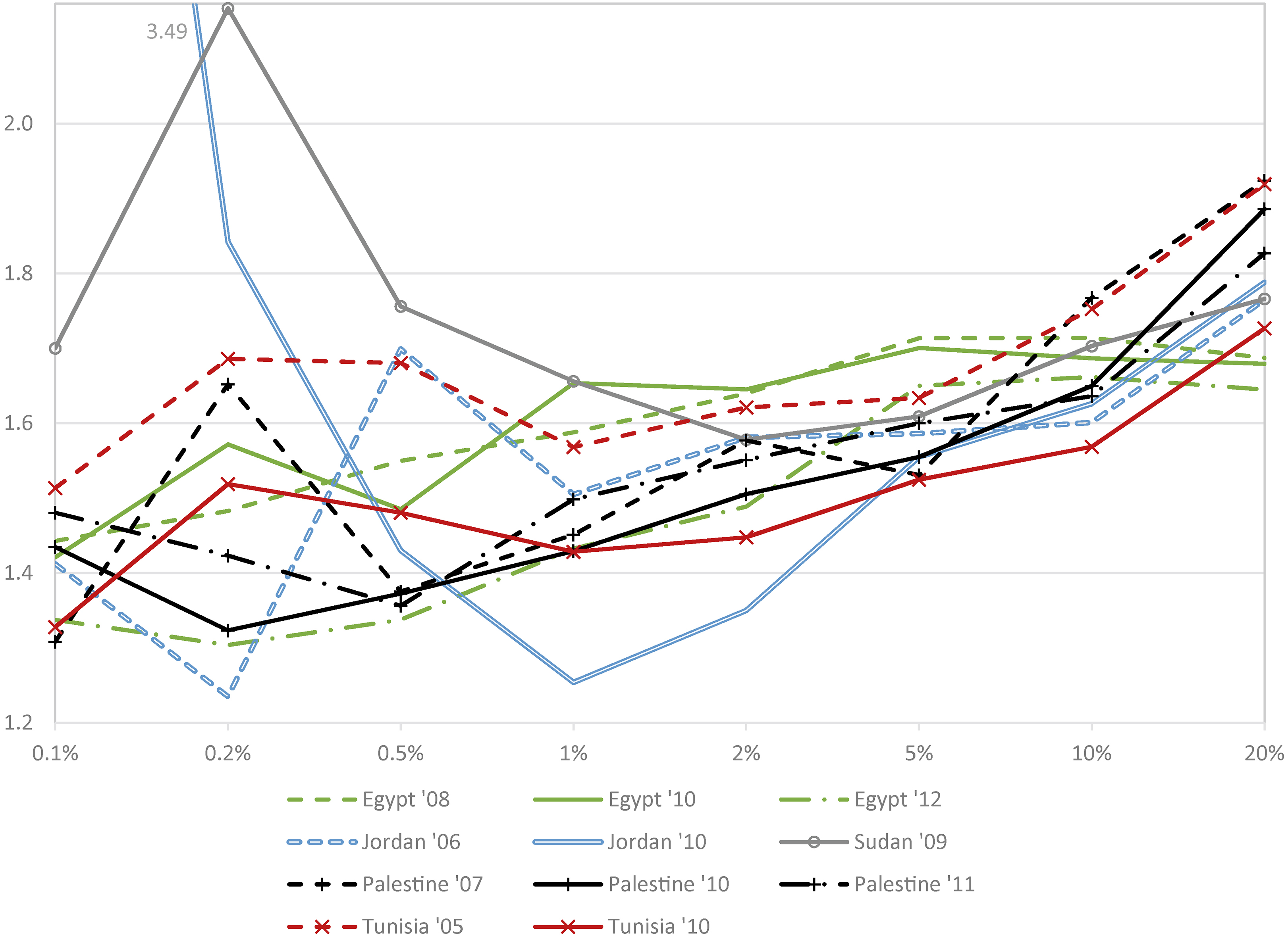

Another measure of dispersion among top expenditures and a measure of the share of aggregate expenditures accounted for by them is the inverted Pareto-Lorenz coefficient, computed as $\beta={\theta}/{(\theta-1)}$ [43]. This coefficient reflects a property of the Pareto law that the ratio of mean expenditure above a threshold for the delineation of top expenditures ( $\overline{x}$ ) to that threshold is constant. The coefficient measures the thickness of the upper tail, and has been found to vary across countries and even over time. Variation in $\beta$ can be explained by changing economic and demographic factors in the population, which affect the topmost expenditures differently than the expenditures of households lower in the distribution (refer to demographic decompositions of inequality by Ramadan et al. [8]). Estimation in Table 2 yields inverted Pareto-Lorenz coefficients of 1.30–1.71 in Egypt, 1.31–1.92 in Palestine, 1.58–2.15 in Sudan, and 1.33–1.92 in Tunisia. In Jordan, the inverted Pareto-Lorenz coefficients are 1.24–1.77 in the 2006 wave and 1.25–3.49 in 2010. These results support our findings that the dispersion of top expenditures is widest in Jordan ‘10 and in Sudan, and least wide in Egypt, followed by Palestine and Tunisia.

In all surveys except Jordan ‘10 and Sudan ‘09, the inverted Pareto-Lorenz coefficient increases nearly monotonically as a greater percentage of top observations are used for estimation and are replaced (refer to Fig. 2). This suggests that as more of lower expenditures are added to the analysis, the degree of dispersion at the top increases as does the expenditure share of the topmost observations. In Egypt and Tunisia, the increase in the inverted Pareto-Lorenz coefficient is timid as 1–20 percent of top expenditures are added (the coefficient stagnates at 1.6–1.7 in Egypt ‘08 and ‘10), suggesting that a Pareto distribution with a single parameter may describe that entire range of top expenditures adequately. On the other hand, in Jordan ‘10, the inverted Pareto-Lorenz coefficient falls drastically from 3.49 when only the top 0.5% of observations are evaluated to 1.25 when top 1% are evaluated. This is clearly due to the single highest influential observation.

Figure 2 disagrees with an observation made by Burkhauser et al. [44], and Alvaredo and Piketty [24] that the inverted Pareto-Lorenz coefficient tends to fall as more of top observations are evaluated. Taking Figs 1 and 2 together, we conclude that extreme observations are not problematic for inequality measurement in our sample of surveys (with the exception of a handful of observations in Jordan ‘10 and Palestine ‘10). Instead, it is the rather narrow dispersion of expenditures between the 80 ${}^{\text{th}}$ and the 95 ${}^{\text{th}}$ percentile (or the top ventile in Egypt) that causes a divergence from what would be expected under the Pareto law.

These findings also suggest that the exact cutoff for expenditures used in the analysis affects the estimated shape of the top expenditure distribution. Different surveys display different sensitivity to the choice. The estimated Pareto coefficient varies by less than 0.4 percentage points in Egypt ‘08 and ‘10 and in Sudan; by 0.7–0.9 in Egypt ‘12, Jordan ‘06 and Tunisia; by 0.8–1.2 in Palestine; and by as much as 2.7 ( $\theta\in[2.27,4.94]$ ) in Jordan ‘10 depending whether at most 1% of the richest households or as many as 20% are evaluated.

The estimated measures of inequality are also affected by the chosen cutoff for top expenditures. The correction for potentially imprecise top expenditures ranges $-$ 0.01–0.43 percentage points of the Gini in Egypt; $-$ 0.81–1.23 percentage points in Jordan; $-$ 0.08–1.95 percentage points in Palestine; $-$ 0.19–0.65 percentage points in Sudan; $-$ 0.05–1.56 percentage points in Tunisia.6 While not trivial, these differences in corrections are modest in size, particularly in view of the size of standard errors on all the Ginis (0.28–2.00). Consequently, individual specifications of the top income distribution (nonparametric, or Pareto parametric distributions estimated from different cutoff points) cannot be clearly rejected in favor of one another. Confidence intervals around the various Pareto estimates and the nonparametric estimates of the Ginis overlap, implying that neither set of estimates can be clearly rejected regardless whether Pareto or nonparametric (or another) type of estimation was appropriate. Figures 1 and 2 illustrate.7

To evaluate whether it was appropriate to model the top expenditures as Pareto distributed, we can compare the estimated Pareto coefficients across different delineations of top expenditures. We can also draw the Hill plots of the estimated distributions, showing how the estimated Pareto parameter changes as one changes the cutoff for top expenditures to a particular percentile [57]. The fit of the Pareto distributions can also be evaluated from the size of standard errors on the Pareto coefficients. If the standard error is large, the estimated Pareto distribution is not very predictive of the dispersion of top expenditures, and alternative Pareto coefficients cannot be effectively tested against one another. Another parametric distribution may represent the dispersion pattern better.

Table 2 shows that the Pareto distributions fitted to top expenditures vary across different delineations of the top expenditures. When the distributions are fitted only among the top 1 percent or fewer observations, the Pareto coefficients vary between 2.5 and 4.0 in Egypt, 1.4–5.3 in Jordan, 3.0–4.2 in Palestine, 1.9–2.5 in Sudan, and 2.5–4.1 in Tunisia. When the fitting is among top 2–20 percent of observations, the Pareto coefficients are notably lower and tighter (see bottom rows of Table 2), at 2.4–2.6 in Egypt, 2.3–3.9 in Jordan, 2.1–3.0 in Palestine, 2.3–2.7 in Sudan, and 2.1–3.2 in Tunisia (refer to Fig. A3). In all surveys but Sudan, the coefficients drift downward nearly monotonically as a greater share of expenditures are used for fitting.

Coefficient standard errors indicate that there is more noise around the estimates when the sample sizes are small, particularly in the Jordanian samples. This suggests that the uppermost observations are not distributed as smoothly as to reflect the Pareto law. The small samples and the presence of outliers may also give rise to estimation bias [39]. The estimates become precise only when at least 2 percent of top observations (47–790 observations or more in our samples) are used for estimation. Using 95% confidence intervals, Pareto coefficients estimated on top 2 percent of expenditures are significantly higher than those estimated on top 20 percent of expenditures in Jordan ‘10, Palestine ‘10, and Tunisia ‘05 and ‘10.8

One motivation for replacing actual top expenditures with synthetic values is to mitigate the sampling error in inequality measurement due to sampling variability across survey waves. Under the conjecture that the true Gini coefficient is stable across nearby years [58], we could expect the quasi-nonparametric Gini to be more stable than the observable nonparametric Gini. Indeed, in most model specifications for Egypt and Jordan, and in one half of model specifications for Palestine and Tunisia (refer to Table 2), the quasi-nonparametric Ginis exhibit less variation over time than the nonparametric Ginis. At the same time, the quasi-nonparametric Ginis carry standard errors that are only 20 percent higher than the nonparametric standard errors, and are of the same size in Sudan ‘09 and lower in Jordan ‘10. This suggests that the method advanced in this study may have distinct benefits over traditional nonparametric estimation of the Gini and its trend over time, particularly in datasets where there are clear outliers.

Finally worth noting, the Pareto and inverted Pareto-Lorenz coefficients and Ginis can be compared to those in prior studies worldwide. Using Atkinson et al.’s [43] estimates, the top expenditures in the five Arab countries considered here have lower inverted Pareto coefficients – and thus exhibit lower dispersion and lower aggregate expenditure shares – than incomes in Argentina, India and even Singapore over the past two decades. They are on par with the inverted Pareto coefficients for incomes in Mediterranean Europe (France, Italy, Portugal, Spain). Even restricting attention to prior estimates for expenditures [26], our five countries exhibit an inverted Pareto coefficient below the median of emerging economies worldwide, or 1.7 (1.8 for income). Even the highest estimates of the inverted Pareto coefficients in our study, when estimated on fully 20 percent of top expenditures, range between 1.64 and 1.92, around the worldwide emerging-countries’ median.

4. Discussion

This study has aimed to evaluate the patterns of dispersion of top expenditures in eleven recent surveys from five Arab countries, and their implications for the measurement of inequality in the region and in emerging countries worldwide. We have attempted to correct the inequality estimates for potentially mismeasured top expenditures. Inspection of the eleven surveys indicates that the topmost expenditures in the Egyptian surveys are distributed fairly narrowly, followed by the Tunisian and Sudanese surveys, while in the Jordanian and Palestinian surveys they are quite dispersed. The 2010 waves of the Jordanian and Palestinian surveys contain clear outliers affecting the measurement of inequality. We thus attempted to correct for such values that are potentially non-representative of the underlying population using values drawn from the expected Pareto distribution.

In our study using only survey data on expenditures, the Gini coefficient is estimated consistently between 0.30 and 0.32 in Egypt, 0.35 to 0.37 in Jordan, and 0.38 to 0.43 in Palestine, Sudan and Tunisia. Replacing observed top expenditures with synthetic values helped to refine the Ginis systematically albeit modestly. Across all surveys, replacing the top 20 percent of expenditures yielded higher Ginis suggesting that in that range of expenditures actual values are dispersed more narrowly than predicted under smooth Pareto distributions (relative to the dispersion of the topmost 0.1–5% of expenditures).

We also found that different countries exhibit different sensitivity to the correction of potentially contaminated top expenditures. In Egypt, followed by Palestine and Tunisia, the estimated inverted Pareto-Lorenz coefficient is near invariant to the cutoff for the delineation of top expenditures, suggesting that Pareto distributions may describe the top expenditures rather well in support of the Pareto law. In Jordan and Sudan the inverted Pareto-Lorenz coefficient fluctuates, suggesting that Pareto distributions do not track the upper tail too closely. Modeling top expenditures in these countries may require a more complex parametric form.

Our estimates of the dispersion of top expenditures (using inverted Pareto coefficients), or all expenditures (using the Ginis) are below or at the mean of the range put forward by Atkinson et al. [43] and Hlásny and Verme [26] for income and expenditure distributions in emerging countries. Particularly in Egypt, inequality is low and falling. Top expenditures in Egypt are distributed rather smoothly and Pareto-like. The falling inequality is thus not due to the presence or absence of extreme observations in any year. The same can be said about the falling inequality in Tunisia, and subject to larger standard errors in Palestine. The trend in Jordan, however, hinges on the inclusion of a few outliers.

Generally, whether the observed or the synthetically derived Ginis are closer to the true degree of inequality in the five countries is unclear, as it depends on the source of the observed dispersion of top expenditures. Differences across the various Gini estimates are also modest in view of their differences across countries. Indeed, nonparametric Ginis vary by as much as 11.8 percentage points across the five countries (29.6 in Egypt ‘12 to 41.4 in Tunisia ‘05). The width of confidence intervals around all estimates – shown in Table 2 and Fig. 1 – implies that neither set of point-estimates can be clearly favored over others.

These conclusions are based on the assumption that the expenditures on which parametric distributions were estimated are not systematically understated. Allowing for this potential problem, the parametric approximations would themselves lead to underestimation. To the extent that there is no clear evidence in existing literature regarding systematic underreporting of expenditures in Arab countries, this method appears appropriate. In fact, claims of underreporting in regional household surveys typically involve incomes, and are based on suspicions rather than on information that underreporting takes place, how much underrepresentation there is, and through which channels it operates.

Alvaredo and coauthors [23, 24] used external data for the tops of income distributions in the region, and derived greater corrections and higher estimates of the Ginis. In the Arab region, however, external data such as national accounts and tax records do not agreed with the survey data on household expenditures, due to issues such as the size of the oil sector, unreported remittances from abroad, neighborhood and family transfers across households, and tax avoidance. Whether household-survey data alone or in combination with national accounts data can provide more relevant estimates of economic inequality is an open question. Moreover, economic inequality across households is also entangled with other dimensions of inequality, such as health inequality, inequality of opportunities, and inequality between countries. All these factors drive a wedge between people’s perceptions and the reality of economic inequality, giving rise to what has been dubbed the Arab inequality puzzle [17].

Our findings regarding the extent of within-country inequality in expenditures thus address only a small part of the puzzle. It is widely recognized that expenditures are distributed more equally than incomes or wealth, due to households’ propensity to save and borrow to smooth consumption, and households’ tendency to recall or report income incorrectly. (Indeed, using disposable incomes in place of expenditures raises the estimates of inequality in all surveys, but upholds the conclusion that inequality fell in Egypt and Palestine – refer to Table A3.) In the Arab region, moreover, consumption tends to be funded by incomes of extended families. Finally worth noting, inequality in households’ expenditures may be systematically biased for inequality in households’ true consumption and welfare, because of systematic differentials in access to free public goods. Poor households face an inadequate public provision of education, health services, and other infrastructure in their communities. They must pay out of pocket to compensate for lacking public transportation, car damage on poorly maintained roads, lack of health/property insurance, or property theft, something that wealthy households do not spend money on. Whether the observed expenditures or incomes are better measures of households’ true welfare thus remains an open question.

Our central finding is that neither the uncorrected Ginis nor the parametric Ginis can be favored over each other on conceptual grounds. We may take our claim further and surmise as follows: under the assumption that nonparametric estimates are consistent for latent true Ginis but potentially inefficient due to a handful of outliers and measurement errors, and that the quasi-nonparametric estimates may be more efficient but potentially inconsistent due to misspecification, similarity of the two sets of estimates suggests that neither measurement errors nor specification errors are sufficiently grave to let us clearly reject either set of the Ginis. For the time being, we should take caution relying on a single estimate, instead considering multiple alternative estimates to construct intervals of plausible values of the countries’ true degrees of economic inequality.

Footnotes

I am grateful to an anonymous referee for making this important point.

Table A1 (and A2) lists the top twenty per-capita expenditure (disposable income, respectively) observations in each survey, representing 0.18–0.31 percent of all households. Several observations can be made: 1) Similar degrees of dispersion are evident across different versions of the Egyptian ‘08 HIECS: the 50% random extraction provided through ERF, the 25% and 50% extractions provided directly by the Egyptian Central Agency for Public Mobilization and Statistics. In the full 100% sample of the ‘08 HIECS (restricted-access), the gap between the richest and second richest household is 54%, and that between the richest and the 20 ${}^{\text{th}}$ richest is 282% (34% and 694%, respectively, for income). 2) In the Jordanian and Palestinian surveys, top expenditures exceed top disposable incomes. Many of these observations are for the same households, reflecting either negative saving rates, high imputed consumption of durables purchased in prior years, or some misreporting of expenditures or income.

This observation is for a three-member household, so the conversion to per-capita terms does not explain the unusual value. Rather, the household includes two earners, one of a very high age. Using an alternative adult-equivalence scale giving lesser weight to the elderly would further increase the expenditure per capita of this household to $324,719. Yet, under this alternative scale, Jordan’s Gini would fall by 2 percentage points. Evaluation of individual expenditure components does not reveal the existence of any data-entry errors for this household. The household’s possession of various household durables confirms the household’s level of wealth. Correspondingly, expenditure on furniture, housing equipment, appliances, transportation vehicles, culture and recreation, energy, miscellaneous goods and various fees are very high. Expenditures on health and medical treatment abroad are also high. Finally, because of its rarity, this household has an above-average sampling weight, implying that it is quite influential in any estimation of population statistics.

We also estimate the distributions on samples right-truncated below values deemed as potentially contaminated by measurement issues. We again find that the topmost observations may be distributed too narrowly compared to what would be expected under the Pareto law (Table A5). Armour et al. [38] apply a similar method using known information on the number of top-coded observationsmathrm; our method is not limited to the case of topcoding, but also allows for general mismeasurement, outliers, or nonresponse. Jenkins [] discusses the appropriate type of Pareto specification and cutoffs for estimation.

These corrections are the differences between nonparametric and quasi-nonparametric Ginis. The quasi-nonparametric Ginis from random draws differ by up to 0.89 percentage points in absolute value from non-randomized smooth-distribution Ginis in Jordanian surveys, by up to 0.45 percentage points in Sudan, and by up to 1.08 percentage points in Tunisian surveys (mean difference in absolute value across these eleven surveys is 0.27 pc.pt.).

While Pareto distribution has been accepted as providing a good fit for income and expenditure distributions, other more flexible statistical distributions have been suggested as providing a potentially better fit, such as the four-parameter GB2 distribution. Table A6, Fig. A2 and the associated text review the results.

Figures A4 and A5 compare actual top expenditures to those predicted under the Pareto distributions estimated among the top 5 or 20 percent of expenditures. Figure A4 again shows the influence of outliers in Jordan ‘10 and Palestine ‘10, the narrow dispersion in the tails in Egypt, and the good fit of this particular Pareto distribution (estimated among the top 5%) in Egypt ‘10, Jordan ‘06, Palestine ‘07 and Sudan ‘09. When the Pareto distributions are estimated among the top 20% of expenditures, the degree of fit further improves in Egypt but deteriorates in other countries. The Hill plots (Fig. A6) show volatile behavior among the topmost 0.2 percent of expenditures in all surveys (6–82 observations in our samples). Beyond this share, the plots for the Egyptian and Palestinian surveys (top row) are near-stationary at a single parameter value across the top 0.5–20% of expenditure observations. Hill plots for the Jordanian, Sudanese and Tunisian surveys (bottom row), on the other hand, slope downward throughout most the range of top expenditures. These Hill plots indicate that a one-parameter Pareto distribution is adequate at approximating the observed top-expenditure distributions in Egypt and Palestine, but not in the other three countries, particularly past 5% of the topmost expenditures. Only in Sudan ‘09 and Tunisia ‘05 the plots are relatively stable and hump-shaped (rather than falling monotonically) until top 5% of the respective samples, suggesting that even in these surveys Pareto approximation may be possible among the top 5% of expenditures.

Conflict of interest

The author declares that he has no conflict of interest.

Supplementary data

The supplementary files are available to download from http://dx.doi.org/10.3233/ JEM-200469.

References

Hlásny

Intini

. Representativeness of top expenditures in Arab region household surveys. UN ESCWA/EDID Working Paper 11; 2015.

Africa Development Bank (AfDB). Jobs, justice and the Arab spring: inclusive growth in north Africa. North Africa Operations Department report; 2012. www.afdb.org/en/documents/document/jobs-justice-and-the-arab-spring-inclusive-growth-in-north-africa-27978 [accessed 2020 Feb 10].

Ncube

Anyanwu

. Inequality and Arab spring revolutions in North Africa and the Middle East. Afr Dev Bank: Afr Econ Brief. 2012; 3(7): 1.

Tessler

Jamal

Robbins

. New findings on Arabs and democracy. J Democr. 2012; 23(4): 89.

Al-Shawarby

. The measurement of inequality in the Arab Republic of Egypt: a historical survey. In: Verme

, et al., eds. Inside inequality in the Arab Republic of Egypt: facts and perceptions across people, time and space. Washington: World Bank; 2014. ch. 1.

Azour

v. Social justice in the Arab world. E/ESCWA/SDD/2014/Background Paper. Beirut: UN ESCWA; 2014.

Gatward

. Economic opportunity and inequality as contributing factors to the Arab spring: the cases of Tunisia and Egypt. Boston College Electronic Thesis; 2015.

Ramadan

Hlásny

Intini

. Inter-group expenditure gaps in the Arab region and their determinants: Application to Egypt, Jordan, Palestine and Tunisia. Rev Inc Wealth. 2018; 64(s1): S145.

Verme

. Facts and perceptions of inequality. In: Verme

, et al., eds. Inside inequality in the Arab Republic of Egypt: facts and perceptions across people, time and space. Washington: World Bank; 2014.

10.

Teti

Abbott

Cavatorta

. The Arab uprisings in Egypt, Jordan and Tunisia: social, political and economic transformations. Berlin: Springer; 2017.

11.

Tobin

. Jordan’s Arab spring: The middle class and anti-revolution. Middle East Policy. 2012; 19(1): 96.

12.

Hinnebusch

. Authoritarian persistence, democratization theory and the Middle East: An overview and critique. Democratization. 2006; 13(3): 373.

13.

Joya

Bond

El-Amine

Hanieh

Henaway

. The Arab revolts against neoliberalism. Center for Social Justice; 2011.

14.

Bogaert

. Contextualizing the Arab revolts: The politics behind three decades of neoliberalism in the Arab world. Mid East Critique. 2013; 22(3): 213.

15.

Dahi

Munif

. Revolts in Syria: Tracking the convergence between authoritarianism and neoliberalism. J Asian & Afr Studies. 2012; 47(4): 323.

16.

Achcar

. The people want: a radical exploration of the Arab uprising. Berkeley: University of California Press; 2013.

17.

Ianchovichina

. Eruptions of popular anger: the economics of the Arab spring and its aftermath. MENA Development Report. Washington: World Bank; 2017.

18.

Bibi

Nabli

. Equity and inequality in the Arab region. ERF Policy Research Report 33. Cairo: Economic Research Forum; 2010.

19.

Bibi

Nabli

. Income inequality in the Arab region: Data and measurement, patterns and trends. Mid East Dev J. 2009; 1(2): 275.

20.

Pinkovskiy

Sala-i-Martin

. Parametric estimations of the world distribution of income. NBER Working Paper 15433; 2009.

21.

Van der Weide

Lakner

Ianchovichina

. Is inequality underestimated in Egypt? Evidence from house prices. Rev Inc Wealth. 2018; 64(s1): S55.

22.

Assouad

. Top income and personal taxation in Lebanon: an exploration of individual tax records. Master’s Thesis. Paris School Econ; 2015.

23.

Alvaredo

Assouad

Piketty

. Measuring inequality in the Middle East 1990–2016: the world’s most unequal region? CEPR Discussion Paper DP12405; 2017.

24.

Alvaredo

Piketty

. Measuring top incomes and inequality in the Middle East: data limitations and illustration with the case of Egypt. ERF Working Paper 832. Cairo: Economic Research Forum; 2014.

25.

Verme

Hlásny

. Top incomes, inequality and the Egyptian case. World Bank Let’s Talk Development blog; 2016. http://blogs.worldbank.org/developmenttalk/eastasiapacific/top-incomes-inequality-and-egyptian-case [accessed 2020 Feb 10].

26.

Hlásny

Verme

. Top incomes and the measurement of inequality in Egypt. World Bank Econ Rev. 2018; 32(2): 428.

27.

Hlásny

Verme

. Top incomes and the measurement of inequality: a comparative analysis of correction methods using EU, US and Egyptian survey data. ECINEQ Working Paper 145; 2015.

28.

Hlásny

Ceriani

Verme

. Bottom incomes and the measurement of poverty and inequality. ERF-LIS Working Paper; 2020.

29.

AlAzzawi

Hlásny

. Household asset wealth and female labor supply in MENA. Q Rev Econ Fin. 2019; 73: 3.

30.

Hlásny

AlAzzawi

. Asset inequality in MENA: The missing dimension? Q Rev Econ Fin. 2019; 73: 44.

31.

El Enbaby

Galal

. Inequality of opportunity in individuals’ wages andhouseholds’ assets in Egypt. ERF Working Paper 942. Cairo: Economic Research Forum; 2015.

32.

Cowell

Victoria-Feser

. Robust Lorenz curves: A semiparametric approach. J Econ Ineq. 2007; 5: 21.

33.

Van Kerm

. Extreme incomes and the estimation of poverty and inequality indicators from EU-SILC. IRISS Working Paper 2007-01, CEPS/INSTEAD doc. 07-07-0335-E; 2007.

34.

Lakner

Milanovic

. Global income distribution from the fall of the Berlin Wall to the great recession. World Bank Policy Research Working Paper 6719; 2013.

35.

Hlásny

. Parametric representation of the top of income distributions: options, historical evidence and model selection. Commitment to Equity Working Paper 90; 2020.

36.

Deaton

. The analysis of household surveys: a microeconometric approach to development policy. Washington: World Bank; 1997.

37.

Krafft

Assaad

Nazier

Ramadan

Vahidmanesh

Zouari

. Estimating poverty and inequality in the absence of consumption data: an application to the Middle East and North Africa. ERF Working Paper 1100. Cairo: Economic Research Forum; 2017.

38.

Armour

Burkhauser

Larrimore

. Using the Pareto distribution to improve estimates of topcoded earnings. Econ Inq. 2016; 54(2): 1263.

39.

Jenkins

. Pareto distributions, top incomes and recent trends in UK income inequality. Economica. 2017; 84(334): 261.

40.

Cowell

Flachaire

. Income distribution and inequality measurement: The problem of extreme values. J Econometr. 2007; 141(2): 1044.

41.

Cowell

Victoria-Feser

. Poverty measurement with contaminated data: A robust approach. Eur Econ Rev. 1996; 40: 1761.

42.

Neri

Gagliardi

Ciampalini

Verma

Betti

. Outliers at upper end of income distribution. (EU-SILC 2007). DMQ Working Paper 86; 2009.

43.

Atkinson

Piketty

Saez

. Top incomes in the long run of history. J Econ Lit. 2011; 49: 3.

44.

Burkhauser

Feng

Jenkins

Larrimore

. Recent trends in top income shares in the United States: Reconciling estimates from March CPS and IRS tax return data. Rev Econ Stat. 2012; 94(2): 371.

45.

Arnold

. Pareto distributions. 2nd ed. New York: CRC Press; 2008.

46.

Levy

Solomon

. New evidence for the power-law distribution of wealth. Physica A: Stat Mech & Appl. 1997; 242(1–2): 90.

47.

Davies

Lluberas

Shorrocks

. Estimating the level and distribution of global wealth, 2000–2014. Rev Inc Wealth. 2017; 63(4): 731.

48.

Vermeulen

. How fat is the top tail of the wealth distribution? Rev Inc Wealth. 2018; 64(2): 357.

49.

Jenkins

Van Kerm

. Paretofit: Stata module to fit a type 1 Pareto distribution. Statistical Software Components S456832. Boston College Department of Economics [revised 11 Nov 2015]; 2007.

50.

Hill

. A simple general approach to inference about the tail of a distribution. Annals Stat. 1975; 3(5): 1163.

51.

Little

RJA

. Multiple imputation: An alternative to top coding for statistical disclosure control. J Royal Stat Soc A. 2007; 170: 923.

52.

Jenkins

Burkhauser

Feng

Larrimore

. Measuring inequality using censored data: A multiple-imputation approach to estimation and inference. J Royal Stat Soc. 2011; 174(1): 63.

53.

Reiter

. Inference for partially synthetic, public use microdata sets. Surv Methodol. 2003; 29: 181.

54.

Hlásny

. Nonresponse bias in inequality measurement: Cross-country analysis using Luxembourg Income Study surveys. Soc Sci Q. 2020; 101(2): 712.

55.

Jenkins

. Gb2lfit: Stata module to fit generalized beta of the second kind distribution by maximum likelihood (log parameter metric). Statistical Software Components S457897. Boston College Department of Economics; 2014.

56.

Scotto

. Hill estimator for the index of regular variation. Stata Tech Bull. 2001; 10(56).

57.

Drees

de Haan

Resnick

. How to make a Hill plot. Annals Stat. 2000; 28: 254.

58.

Squire

Zou

. Explaining international and intertemporal variations in income inequality. Econ J. 1998; 108(446): 26. The following datasets were accessed in the Harmonized Household Income and Expenditure Surveys (HHIES) database at Egypt-based Economic Research Forum’s (ERF) portal: www.erf.org.eg/cms.php?id=erfdataportal [accessed 2020 Feb 10]:

59.

Open Access Micro Data Initiative (OAMDI). Version 2.0 of licensed data files. HIECS 2008/2009 – Central Agency for Public Mobilization and Statistics; 2014a.

60.

OAMDI. Version 2.0 of licensed data files; HIECS 2010/2011 – Central Agency for Public Mobilization and Statistics; 2014b.

61.

HIECS 2012/2013 – Central Agency for Public Mobilization and Statistics; 2014c.

62.

OAMDI. Version 2.0 of licensed data files; HEIS 2006 – DOS, Hashemite Kingdom of Jordan; 2014d.

63.

Economic Research Forum and the Department of Statistics of Hashemite Kingdom of Jordan (ERF & DOS). Household expenditure and income survey 2010/2011 (HEIS 2010/2011), Version 1.0 of the Licensed data files, March 2013. DOS, Hashemite Kingdom of Jordan; 2013.

64.

OAMDI. Version 2.0 of licensed data files; PECS 2007 – Palestinian Central Bureau of Statistics; 2014e.

65.

OAMDI. Version 2.0 of licensed data files; PECS 2010 – Palestinian Central Bureau of Statistics; 2014f.

66.

OAMDI. Version 2.0 of licensed data files; PECS 2011 – Palestinian Central Bureau of Statistics; 2014g.

67.

OAMDI. Version 2.0 of licensed data files; NBHS 2009 – Central Bureau of Statistics, Sudan; 2014h.

68.

OAMDI. Version 2.0 of licensed data files; EBCNV 2005 – National Institute of Statistics, Tunisia; 2014i.

69.

OAMDI. Version 2.0 of licensed data files; EBCNV 2010 – National Institute of Statistics, Tunisia; 2014j.

Top expenditure distribution in Arab countries and the inequality puzzle 1

Abstract

Keywords

1. Introduction

2. Survey data, right-tail measurement issues, and correction methods

2.1 Available data

Table 1 Data sources and summary statistics

2.3 Replacement using values from a Pareto distribution

Table 2 Quasi-nonparametric estimates of Gini coefficients: Pareto distribution

Footnotes

Conflict of interest

Supplementary data

References

Table 1
Data sources and summary statistics

Table 2
Quasi-nonparametric estimates of Gini coefficients: Pareto distribution