Revisiting taste change in cost-of-living measurement

Abstract

This paper compares conditional and unconditional cost-of-living indexes (COLI) when tastes change, focusing on the Constant Elasticity of Substitution model. A consumer price index typically targets a conditional COLI, which evaluates price change given set of preferences. An unconditional COLI aims to also capture the welfare effects of changing tastes, but it requires stronger assumptions. Using retail scanner data for food and beverage products, I find COLIs conditioning on current period tastes exceed those conditioning on prior period tastes. Consistent with previous studies, I find an unconditional COLI tends to reflect negative direct contributions from taste change.

Keywords

Cost of living index price index taste change

1. Introduction

A cost-of-living index (COLI) is based on the expenditure function from classical consumer theory. The evolution of expenditures over time may reflect changes in many factors in addition to prices. Preferences (which may also be referred to as tastes) may themselves be influenced by climate, crime, or fashion, to name a few. Index users may wish to account for preferences in different ways. Users of a consumer price index (CPI), for instance, may not want to adjust payments (for example) in response to non-price factors. For reasons like this, the target of a CPI is commonly (though not universally) agreed to be a conditional COLI, which holds preferences fixed [1, 2]. For example, the Tornqvist formula used by the Bureau of Labor Statistics (BLS) for the U.S. Chained Consumer Price Index for All Urban Consumers (C-CPI-U) approximates the conditional COLI pertaining to the set of average tastes [3]. On the other hand, researchers may be interested in how changing prices and changing preferences combine to impact an unconditional COLI. Notably, Redding and Weinstein [4] (henceforth RW), find using household scanner data that changing preferences lower costs of living significantly.

This paper reviews the literature on COLI measurement in the presence of taste change and compares the conditional and unconditional COLI approaches theoretically and empirically. The empirical analysis focuses on the Constant Elasticity of Substitution (CES) model. The CES model is widely used in cost-of-living analysis, including studies of preference change. It allows for price-related substitution effects, and traditional price index formulas like the Laspeyres, Paasche, and Cobb-Douglas correspond to special or limiting cases [2]. A CES index is also used for initial estimates of the C-CPI-U [5]. The indexes I consider are for the most part well-known in the literature, though some, like the Lloyd [6] and Moulton [7] variants, have not been widely discussed in the context of conditional COLIs nor estimated alongside unconditional COLIs. While there has been a recent literature on taste change exemplified by RW, it focuses primarily on unconditional COLIs. Among others, Hottman and Monarch [8] and Ueda et al. [9] also explore indexes of the unconditional type. Many earlier studies of taste change (e.g. Phlips and Sanz-Ferrer [10]; Heien and Dunn [11]) either use a model other than CES, a specific parameterization of the taste change, or allow taste changes for a small subset of products.

A few key themes emerge from the analysis which may be of use to practitioners. First, conditional COLIs generally depend on the indifference surface at which they are measured, and average tastes might not be the only interesting reference point for price-level comparisons, particularly if tastes are changing rapidly. Using retail scanner data for food and beverage products, I estimate that COLIs conditioning on current period tastes exceed those conditioning on past tastes by an average of 0.6 to 3.0 percentage points per year, depending on the product category, with COLIs conditioning on intermediate tastes falling roughly in the middle. Faced with different conditional COLIs, a researcher may desire a single estimate that does not give primacy to one period’s tastes. Notably, I find it matters little whether they condition on intermediate tastes (an interpretation of the index of Sato [12] and Vartia [13]) or simply average the past and current taste conditional COLIs. Accounting for tastes at the individual product level is infeasible within current data constraints at the BLS. However, in Appendix A.2, I find that aggregates of U.S. CPI data that similarly account for broader item-stratum level tastes are affected to a lesser extent by the choice of taste vector than are the detailed product group indexes formed using the retail data.

Unconditional COLIs deliver a potentially more comprehensive measure, though at a cost of imposing stronger assumptions on preferences. The latter point has not been widely discussed in the recent literature. Incorporating the direct effects of preference change necessarily treats utility as cardinal [14] and requires a restriction on the taste change process. Under these assumptions and using RW’s method, I find the unconditional COLI is, on average, within 0.05 percentage points per year of a COLI that conditions on past preferences. I also find the unconditional COLI averages 1.1 percentage points lower than a COLI that conditions on average tastes. This is qualitatively similar to concurrent findings in Ehrlich et al [15] and is of the same sign, though of a larger magnitude than RW. RW interpret this wedge as a “taste-shock bias” which afflicts indexes like the Tornqvist or Sato-Vartia which do include direct taste effects. However, it might validly be interpreted as reflecting the distinct theoretical targets of the indexes in question. With available items tending to change over time, the unconditional COLI estimate is more sensitive (relative to the conditional COLIs) to which items are considered to be “common” to the periods being compared.

2. Existing literature

The economic approach to consumer price indexes, dating to Konüs [16], is based on the expenditure function of an optimizing agent. The final version of the C-CPI-U, for example, uses the Tornqvist formula for upper-level aggregation [17]. The Tornqvist is an example of a “superlative” index [18], meaning it approximates an arbitrary expenditure function. The seminal work of Fisher and Shell [19] analyzes conditional and unconditional COLIs in an environment with changing preferences. Follow-up studies by Muellbauer [20], Phlips and Sanz-Ferrer [10], Heien and Dunn [11], among others, explore conditional and unconditional COLI for different models under various assumptions about tastes. This paper highlights methods for estimating conditional COLI for the CES model. The main focus of the paper is CES, but Appendix A.5 derives conditional COLIs for the translog model (which underlies the Tornqvist index). The appropriate target for a consumer price index is generally considered to be a conditional COLI [1, 2], which isolates the effect of changing prices by holding preferences (or anything else affecting well-being) fixed. By referencing a specific indifference surface, a conditional COLI requires only the ordinal properties of utility functions.

An unconditional COLI, on the other hand aims to track changes in expenditure whether driven by price change or preference change. As a consequence, the index may increase or decrease even if prices are constant. An unconditional COLI must reference a cardinal utility level in order to compare expenditures across varying indifference maps. For this reason, unconditional COLI are sometimes called “cardinal,” whereas conditional COLI are sometimes called “ordinal” [20]. Furthermore, because utility is only identified up to a positive monotone transformation, a normalization or restriction on the taste change process is required for index calculation [20]. In RW, the unweighted geometric mean of the taste parameters is assumed to be time constant. Kurtzon [21] explores the robustness of RW’s method to this normalization. Ueda et al. [9] also uses the CES model. Taste changes (which are called fashion effects) are only allowed in the first $\tau$ periods after a product’s introduction, and follow stationary functions of the product’s age. While not a normalization per se, this restriction allows the fashion effects to be accounted for by product turnover adjustments using Feenstra’s method [22], while the remaining fixed-taste component of the COLI is estimated using a Sato-Vartia index over the remaining set of common varieties. Section 4 shows conditional COLIs do not require either restriction. Interested in an unconditional-like COLI concept, but wishing to avoid these drawbacks, Balk [14] proposes an index that attempts to hold constant some notion of well-being without fixing the cardinal utility level. The method tracks the change in expenditure required to reach the period-specific indifference surface that passes through a fixed bundle. Gábor-Tóth and Vermeulen [23] apply this method to European scanner data and find the average annual contribution of taste change to be $-$ 1.1 percentage points. Unconditional COLI seek to answer interesting questions, and may be more comprehensive as cost-of-living concepts. However, they do not contain any additional information on prices than what is already conveyed by a conditional COLI [2].

As noted by Fisher and Shell [19], deriving the relationship between preference change and either type of COLI is difficult without either assuming a specific parameterization (allowing changes on a small subset of items only), or restricting attention to a particular utility function (as this paper does). Tastes do not pose much of a measurement challenge when the objective is a conditional COLI, however, and average tastes are an acceptable reference point. Caves et al. [3], Diewert [24], and Feenstra and Reinsdorf [25] provide conditions under which the Tornqvist, Fisher, and Sato-Vartia price indexes, respectively, are exact for or approximate COLI that condition on some notion of average tastes. Section 3 discusses these results further, while Section 4 complements them by showing that variants of the Lloyd-Moulton index are also exact for conditional COLIs in the CES case. Considering a constant tastes model, Balk [26] and Melser [27] use the theoretical equivalence among these CES-based indexes to back out estimates of the elasticity of substitution. With changing preferences, however, we should expect these indexes to vary as they each correspond to a different conditional COLI.

In order to isolate the issue of preference change, I focus my empirical analysis on matched-model indexes, i.e., those defined over a fixed set of specific product varieties with constant tangible attributes. RW’s taste-shock bias is defined in association with a matched-model index. This is not to suggest that improvements to a matched model index should not be pursued for reasons of representativity. For instance, product turnover can cause matched model indexes to miss initial price declines for new items [22], as well as selection bias in the set of matched items [28]. Applying Feenstra [22], Appendix A.3 shows how with product turnover, the matched model component of the CES conditional COLI is unchanged, and it is possible to bound the variety adjustment term. Preference change is also fundamentally different from quality change, though the two may have similar effects on relative demand. Price change for the matched model is measurable without quality adjustment, since the set of items and their associated bundles of attributes are constant by definition. Though the two issues are similar mechanically [19], taste-shock bias should not be confused with quality bias. If item definitions are not constant, then whether or not demand shifts are attributed to quality changes or taste changes can have large effects on index estimation [29].

3. Cost-of-living theory

It is helpful to first review the cost-of-living index theory and precisely state what conceptual target a price index is intended to measure when preferences are changing. A cost-of-living index is a ratio of two expenditure functions. It is helpful in this case to first specify a set of preferences rather than jump straight to a utility function. Consider an ordinal preference relation, denoted $\succeq$ , on a commodity space $\mathcal{Q}\subseteq\mathbb{R}_{+}^{N}$ , which is made up of bundles $\bm{q}$ . We assume:

Assumption 1. (Ordinal Preferences) A preference relation $\succeq$ is i) rational (complete and transitive), ii) continuous, iii) convex, and iv) monotone.

Assumption 1 is sufficient for the existence of a function, $u:\mathcal{Q}\rightarrow\mathbb{R}$ which represents $\succeq$ , in the sense that we have $\bm{q}\succeq\bm{q}^{\prime}\Leftrightarrow u(\bm{q};\succeq)\geqslant u(\bm{q% }^{\prime};\succeq)$ [30]. Due to the ordinal nature of preferences, the function $u$ , is not unique. Even when assuming a specific form for $u$ (as in Section 4) the most that Assumption 1 would imply about an actual “utility-generating process” is that it follows a function $v=f\circ u$ for some unknown monotonic transformation $f$ .

Let $\bm{p}$ denote a vector of prices. We then assume:

Assumption 2. (Optimization) Facing prices $\bm{p}$ and having preferences $\succeq$ that satisfy Assumption 1, a representative consumer chooses $\bm{q}$ to maximize utility $u(\bm{q};\succeq)$ subject to a budget constraint, or equivalently, to minimize expenditure subject to a utility constraint.

Let $\bm{h}(\bm{p},\bar{u};\succeq)=\underset{\bm{q}}{\text{ argmin }}\bm{p}\cdot% \bm{q}\text{ s.t. }u(\bm{q};\succeq)\geqslant\bar{u}$ denote the Hicksian demand function, which represents the quantities that minimize expenditure. The expenditure function is given as $C(\bm{p},\bar{u};\succeq)=\bm{p}\cdot\bm{h}(\bm{p},\bar{u};\succeq)$ .

The task of the price statistician is to compare price vectors across situations. Following price index convention, I label the reference situation 0 and the comparison situation 1. This paper focuses on bilateral, intertemporal comparisons, but the general theory accommodates other possibilities (e.g., regional comparisons). I maintain Assumptions 1 and 2 separately for both situations (i.e., $C(\bm{p}_{t},\bar{u};\succeq_{t})=\bm{p}_{t}\cdot\bm{h}(\bm{p}_{t},\bar{u};% \succeq_{t})$ , $t=0,1$ ) but take no stand on whether $\succeq_{0}=\succeq_{1}$ unless stated explicitly. In the general case of varying preferences, the cost-of-living framework yields different measurement concepts, which I review in the following subsections.

3.1 Conditional COLI

A conditional COLI is defined as the minimum expenditure required for an agent to be indifferent between two price situations.

.

[19, 31] The class of conditional cost-of-living indexes is given by:

$\displaystyle\Phi(\bm{p}_{0},\bm{p}_{1},\bar{u};\succeq)=\frac{C(\bm{p}_{1},% \bar{u};\succeq)}{C(\bm{p}_{0},\bar{u};\succeq)},$ (1)

for a given $\bar{u}$ and $\succeq$ .

The combination of $\succeq$ (preference relation) and $\bar{u}$ (location) determine the specific indifference surface on which $\Phi$ is based. COLIs are not unique except in special cases like constant, homothetic preferences. As noted by Fisher and Shell [19], unless preferences are constant, a conditional COLI does not equal the compensation required to maintain a constant “standard of living” or utility, as COLIs are often described. Such a measurement is not generally possible under Assumptions 1 and 2.

Two immediate candidates for preferences to plug in are $\succeq_{0}$ and $\succeq_{1}$ . It is worth emphasizing that the oft-cited bounding results for the Laspeyres and Paasche indexes are one-way only, i.e., the Laspeyres is an upper bound for $\Phi(\bm{p}_{0},\bm{p}_{1},u_{0};\succeq_{0})$ , and the Paasche is a lower bound for $\Phi(\bm{p}_{0},\bm{p}_{1},u_{1};\succeq_{1})$ , where $u_{t}=u(\bm{q}_{t},\succeq_{t})$ for $t=0,1$ . Fisher and Shell [19] argue that from the standpoint of intertemporal compensation, the most interesting COLI is

$\displaystyle\Phi(\bm{p}_{0},\bm{p}_{1},\bar{u}_{1}^{*};\succeq_{1})=\frac{C(% \bm{p}_{1},\bar{u}_{1}^{*};\succeq_{1})}{C(\bm{p}_{0},\bar{u}_{1}^{*};\succeq_% {1})},$ (2)

where $\bar{u}_{1}^{*}$ is the hypothetical utility that the consumer would receive facing the period 0 budget constraint with period 1 preferences. Fisher and Shell [19] and others argue that a COLI based on $\succeq_{1}$ is more relevant for public policy than one based on the obsolete preferences $\succeq_{0}$ , but Pollak [31] notes that in principle, $\succeq$ need not be linked to either the reference or comparison situations. Indeed, two of the parameter-free price indexes discussed in the next subsection are exact for COLI based on average indifference surfaces.

3.2 Parameter-free COLI

Under Assumption 2, the observed market expenditures $\bm{p}_{0}\cdot\bm{q}_{0}$ and $\bm{p}_{1}\cdot\bm{q}_{1}$ equal the expenditure levels $C(\bm{p}_{0},u_{0},\succeq_{0})$ and $C(\bm{p}_{1},u_{1},\succeq_{1})$ , respectively. Since, Eq. 1 holds the indifference surface fixed, however, estimation generally requires knowledge of the expenditure function for the given set of preferences.

Nevertheless, some well-known price index formulas either approximate or are exact for conditional COLI, precluding any need for structural estimation. A price index formula is considered exact if it equals a ratio of expenditure functions for a given model [18]. These indexes and their components are defined below. Let $i$ index items or varieties, and denote the set of items as $\mathcal{I}$ , which has dimension $N$ .

.

The Fisher price index

$\displaystyle P_{F}(\bm{p}_{0},\bm{p}_{1},\bm{q}_{0},\bm{q}_{1})=\sqrt{P_{L}P_% {P}},$ (3)

where $P_{L}(\bm{p}_{0},\bm{p}_{1},\bm{q}_{0},\bm{q}_{1})=\frac{\sum_{i\in\mathcal{I}% }p_{i1}q_{i0}}{\sum_{i\in\mathcal{I}}p_{i0}q_{i0}}$ is the Laspeyres index, and $P_{P}(\bm{p}_{0},\bm{p}_{1},\bm{q}_{0},$ $\bm{q}_{1})=\frac{\sum_{i\in\mathcal{I}}p_{i1}q_{i1}}{\sum_{i\in\mathcal{I}}p_% {i0}q_{i1}}$ is the Paasche index.

.

The Tornqvist price index

$\displaystyle P_{T}(\bm{p}_{0},\bm{p}_{1},\bm{q}_{0},\bm{q}_{1})=\prod_{i\in% \mathcal{I}}\left(\frac{p_{i1}}{p_{i0}}\right)^{0.5(s_{i0}+s_{i1})},$ (4)

where $s_{it}=\frac{p_{it}q_{it}}{\sum_{j\in\mathcal{I}}p_{jt}q_{jt}},t=0,1.$

.

The Sato-Vartia price index

$\displaystyle P_{\textit{SV}}(\bm{p}_{0},\bm{p}_{1},\bm{q}_{0},\bm{q}_{1})=% \prod_{i\in\mathcal{I}}\left(\frac{p_{i1}}{p_{i0}}\right)^{w_{i}},$ (5)

where

$\displaystyle w_{i}=\left[\left.\frac{s_{i1}-s_{i0}}{\ln s_{i1}-\ln s_{i0}}% \right]\right/\left[\sum_{k\in\mathcal{I}}\frac{s_{k1}-s_{k0}}{\ln s_{k1}-\ln s% _{k0}}\right].$

Suppose tastes (or environmental variables, as referred to in Diewert [24], 2001) are represented by the vector of parameters $\bm{\varphi}$ , and that $u()$ is continuous and increasing in $\bm{\varphi}$ , as will be the case in the following section on CES preferences. Then Diewert [24] showed that there exists a $u^{*}$ and $\bm{\varphi}^{*}$ such that $\Phi(\bm{p}_{0},\bm{p}_{1},u^{*};\bm{\varphi}^{*})$ is bounded by the Laspeyres and Paasche indexes, where $u_{0}\leqslant u^{*}\leqslant u_{1}$ and $\varphi_{i0}\leqslant\varphi_{i}^{*}\leqslant\varphi_{i1}$ , $i\in\mathcal{I}$ . If the Laspeyres and Paasche are close numerically, a symmetric average like the Fisher index approximates this COLI. In addition, under the assumption that the expenditure function is translog, Caves et al. [3] showed that the Tornqvist price index is exact for the geometric average of the COLI based on period 0 preferences and the COLI based on period 1 preferences. Due to translog functional form, this is equivalent to the COLI evaluated at the geometric averages of the taste parameters and utilities, respectively. The Tornqvist index is also attractive because the translog expenditure function approximates arbitrary expenditure functions to the second order. Finally, the Sato-Vartia index is exact for the CES COLI that conditions on intermediate levels of the tastes [25]. Each of these results relates to an indifference surface that is, loosely speaking, an average of the base and current period indifference surfaces. Of course, the measurement of substitution effects (responses to relative price change), may change depending on which indifference surface the COLI is based, and so interpretations should be made carefully.

3.3 Unconditional COLI

An unconditional COLI measures the change in expenditure required for the consumer to achieve the same standard-of-living, or utility level, in the comparison period as they experienced in the reference period.

.

[20] The class of unconditional or cardinal COLI is given by:

$\displaystyle\Phi_{U}(\bm{p}_{0},\bm{p}_{1},\bar{u};\succeq_{0},\succeq_{1})=% \frac{C(\bm{p}_{1},\bar{u};\succeq_{1})}{C(\bm{p}_{0},\bar{u};\succeq_{0})},$ (6)

for some $\bar{u}$ .

As discussed by Fisher and Shell [19], shifting preferences complicate the “constant standard-of-living” interpretation of Definition 5. In addition to Assumptions 1 and 2, this interpretation implicitly assumes location $\bar{u}$ under $\succeq_{0}$ is comparable to location $\bar{u}$ under $\succeq_{1}$ (utility is cardinal). In general, the associated quantities $\bm{h}(\bm{p}_{0},\bar{u};\succeq_{0})$ and $\bm{h}(\bm{p}_{1},\bar{u};\succeq_{1})$ lie on different indifference surfaces, even though both are labeled $\bar{u}$ . As utility levels are not identified, normalizations are needed to pin down the relative expenditures associated with maintaining $\bar{u}$ utils. Section 4.2 and Appendix A.4 discuss these further for the CES model.

As discussed in Sections 1 and 2, the unconditional COLI aims to account for the effect of non-price factors on standards of living. This can be illustrated through the following algebraic relationship, which is similar to decompositions in Balk [14] and Gábor-Tóth and Vermeulen [23].

$\displaystyle\ln\Phi_{U}(\bm{p}_{0},\bm{p}_{1},\bar{u};\succeq_{0},\succeq_{1}% )=\ln\Phi(\bm{p}_{0},\bm{p}_{1},\bar{u};\succeq_{1})+\ln\left[\frac{C(\bm{p}_{% 0},\bar{u};\succeq_{1})}{C(\bm{p}_{0},\bar{u};\succeq_{0})}\right]$ (7)

Equation (7) decomposes the unconditional COLI of Definition 5 into two parts; a price effect equal to a conditional COLI, and a pure taste change effect $C(\bm{p}_{0},\bar{u};\mbox{$\succeq_{1}$)}/C(\bm{p}_{0},\bar{u};\succeq_{0})$ . It is straightforward to compare the unconditional COLI with other conditional COLI in a similar fashion. Equation (7) describes the sense in which $\Phi_{U}$ is “unconditional” in that the last term aims to capture the impact of factors other than prices [1]. It is also apparent that the contribution of price change is completely captured by the conditional index, and that the pure taste change component is what requires cardinal utility. If one defines an unconditional COLI using an alternative notion of “constant well-being”, as in Balk [14] then a pure taste change component can be estimated without cardinal utility.

4. CES preferences

Section 3 described a few conditional COLI that can be estimated with prices and quantities only. In general, however, estimating a COLI requires specifying and estimating a model of preferences. For comparability to other studies, I focus on the CES model for the rest of this paper. The CES model is a workhorse for its tractability, though it implies significant restrictions on price and income elasticities. Appendix A.5 derives similar results for the homothetic translog expenditure function, which is more flexible, but requires estimating many more parameters. Specification error is a potential issue for an unconditional COLI, as well as COLI that condition on a specific period’s tastes, as these depend on the model’s ability to separate price responses from preference shifts [32]. While the price indexes considered in this section are not new, some of their relationships with specific conditional COLI when tastes are changing have not been widely discussed in the literature.

We now assume:

Assumption 3. The representative agent’s expenditure function has the form:

$\displaystyle C(\bm{p},\bar{u};\bm{\varphi})=\bar{u}\left[\sum_{i\in\mathcal{I% }}\left(\frac{p_{i}}{\varphi_{i}}\right)^{1-\sigma}\right]^{\frac{1}{1-\sigma}}$ (8)

For the purposes of a COLI, we take $\bar{u}=1$ without further loss of generality (preferences are homothetic) and suppress the argument from further notation. The parameter $\sigma\neq 1$ is the elasticity of substitution, which we assume is constant over time, and so the notation now refers to preferences through the vector of demand shifters $\bm{\varphi}$ . I use $\bm{\varphi}$ to refer to a generic vector, while $\bm{\varphi}_{t}$ refers to the actual preferences of time $t$ . The agent’s optimal expenditure shares are given by

$\displaystyle s_{i}(\bm{p};\bm{\varphi})=\frac{p_{i}h_{i}(\bm{p};\bm{\varphi})% }{\sum_{j\in\mathcal{I}}p_{j}h_{j}(\bm{p};\bm{\varphi})}=\frac{\left(p_{i}/% \varphi_{i}\right)^{1-\sigma}}{\sum_{j\in\mathcal{I}}\left(p_{j}/\varphi_{j}% \right)^{1-\sigma}}=\frac{\left(p_{i}/\varphi_{i}\right)^{1-\sigma}}{\left[C(% \bm{p};\bm{\varphi})\right]^{1-\sigma}},\,i=1,\dots,N.$ (9)

Under Assumptions 2 and 3, the observed expenditure shares $s_{it}=\frac{p_{it}q_{it}}{\sum_{j\in\mathcal{I}}p_{jt}q_{jt}}$ equal the optimal expenditure shares $s_{i}(\bm{p}_{t};\bm{\varphi}_{t})$ . The indexes in the following subsections make use of this equation to estimate conditional and unconditional COLI.

Equation (10) shows that under Assumption 3, the log expenditure share of item $i$ in period $t$ can be decomposed into its log price, the log expenditure function, and the log of the taste parameters.

$\displaystyle\ln s_{it}=(1-\sigma)\ln p_{it}+(\sigma-1)\ln\left[c(\bm{p}_{t};% \bm{\varphi}_{t})\right]+(\sigma-1)\ln\varphi_{it}$ (10)

As RW note, the taste parameters provide a source of idiosyncratic error which is necessary for empirical analysis.

4.1 Exact price indexes for CES preferences

As previously mentioned, the index proposed by Sato [12] and Vartia [13] (see Eq. (5)) is exact for the CES COLI that conditions on an intermediate taste vector $\bar{\bm{\varphi}}$ [25]. Each element $\bar{\varphi}_{i}$ of $\bar{\bm{\varphi}}$ lies between $\varphi_{i0}/\prod_{i\in\mathcal{I}}\varphi_{i0}^{w_{i}}$ and $\varphi_{i1}/\prod_{i\in\mathcal{I}}\varphi_{i1}^{w_{i}}$ . The salient question then is how do price comparisons using $\bar{\bm{\varphi}}$ compare to price comparisons using $\bm{\varphi}_{0}$ , $\bm{\varphi}_{1}$ or some other tastes? Exact price indexes for reference period or current period tastes already exist for the CES model, though to my knowledge, their interpretation as such is novel. Lloyd [6] and Moulton [7] developed the following price index in the setting of constant tastes.

.

Lloyd-Moulton Index

$\displaystyle P_{LM}(\bm{p}_{0},\bm{p}_{1},\bm{q}_{0},\bm{q}_{1},\sigma)=\left% \{\sum_{i\in\mathcal{I}}s_{i0}\left(\frac{p_{i1}}{p_{i0}}\right)^{1-\sigma}% \right\}^{\frac{1}{1-\sigma}}$ (11)

Similarly, the time-antithesis [33], or “backwards” version of the Lloyd-Moulton index can be formed [6].

.

Backwards Lloyd-Moulton Index

$\displaystyle P_{BLM}(\bm{p}_{0},\bm{p}_{1},\bm{q}_{0},\bm{q}_{1},\sigma)=% \left\{\sum_{i\in\mathcal{I}}s_{i1}\left(\frac{p_{i0}}{p_{i1}}\right)^{1-% \sigma}\right\}^{\frac{-1}{1-\sigma}}$ (12)

The Lloyd-Moulton and Backwards Lloyd-Moulton are exact for the COLI that condition on reference period tastes and comparison period tastes, respectively. To see this, start with Eq. (6) for $P_{LM}(\bm{p}_{0},\bm{p}_{1},\bm{q}_{0},\bm{q}_{1},\sigma)$ . Use the right hand side of Eq. (9) to substitute for $s_{i0}$ , re-arrange, and use Eq. (8). We then have

$\displaystyle P_{LM}(\bm{p}_{0},\bm{p}_{1},\bm{q}_{0},\bm{q}_{1},\sigma)=\left% \{\sum_{i\in\mathcal{I}}s_{i0}\left(\frac{p_{i1}}{p_{i0}}\right)^{1-\sigma}% \right\}^{\frac{1}{1-\sigma}}=\left\{\sum_{i\in\mathcal{I}}\frac{\left(p_{i0}/% \varphi_{i0}\right)^{1-\sigma}}{\left[C(\bm{p}_{0},\bm{\varphi}_{0})\right]^{1% -\sigma}}\left(\frac{p_{i1}}{p_{i0}}\right)^{1-\sigma}\right\}^{\frac{1}{1-% \sigma}}=\frac{\left\{\sum_{i\in\mathcal{I}}\left(p_{i1}/\varphi_{i0}\right)^{% 1-\sigma}\right\}}{C(\bm{p}_{0},\bm{\varphi}_{0})}^{\frac{1}{1-\sigma}}=\frac{% C(\bm{p}_{1},\bm{\varphi}_{0})}{C(\bm{p}_{0},\bm{\varphi}_{0})}=\Phi(\bm{p}_{0% },\bm{p}_{1};\bm{\varphi}_{0})$

The case of $P_{BLM}(\bm{p}_{0},\bm{p}_{1},\bm{q}_{0},\bm{q}_{1},\sigma)$ is very similar.

Faced with these two options for conditional COLIs, a price researcher may not wish to give primacy to either period’s preferences. An additional possibility for the case of CES preferences is to calculate the geometric mean of the Lloyd-Moulton indexes, which is exact for the geometric mean of two CES conditional COLI. This index, which I label $P_{\textit{LMM}}$ , has the form:

$\displaystyle P_{\textit{LMM}}(\bm{p}_{0},\bm{p}_{1},\bm{q}_{0},\bm{q}_{1},% \sigma)=\left[P_{LM}(\bm{p}_{0},\bm{p}_{1},\bm{q}_{0},\bm{q}_{1},\sigma)P_{% \textit{BLM}}(\bm{p}_{0},\bm{p}_{1},\bm{q}_{0},\bm{q}_{1},\sigma)\right]^{% \frac{1}{2}}=\left[\frac{\sum_{i\in\mathcal{I}}s_{i0}\left(\frac{p_{i1}}{p_{i0% }}\right)^{1-\sigma}}{\sum_{i\in\mathcal{I}}s_{i1}\left(\frac{p_{i0}}{p_{i1}}% \right)^{1-\sigma}}\right]^{\frac{1}{2(1-\sigma)}}$ (13)

As pointed out in Balk [26] and de Haan et al. [34], Eq. (13) shows $P_{\textit{LMM}}$ is, in fact, the Quadratic Mean of Order $r$ price index, where $r=2(1-\sigma)$ [18]. This is attractive because superlative indexes like this one have been shown to approximate each other to the second order, provided that $|\sigma|$ is not too large [35, 36]. This implies $P_{\textit{LMM}}$ should be somewhat robust to errors in estimation of $\sigma$ or departures from CES functional form.

Additionally, the availability of both $P_{\textit{LMM}}$ and $P_{\textit{SV}}$ for the CES case offers an interesting potential contrast. One averages COLI evaluated at different tastes, while the other is a COLI evaluated at an average of the tastes. A priori, we would not necessarily expect them to give identical answers, though their estimates in Section 5 are very similar.

4.2 RW’s CES common varieties index

RW propose a price index to target the CES unconditional COLI. A practical challenge concerns the scale of tastes. Given knowledge of $\sigma$ , Eq. (9) implies that observed expenditure shares and prices only identify $\varphi_{it}$ up to a time-varying scale factor. RW address this issue by assuming the $\varphi_{it}$ have a constant geometric mean over time.

Assumption 4.

$\displaystyle\prod_{i\in\mathcal{I}}\varphi_{i0}^{1/N}=\prod_{i\in\mathcal{I}}% \varphi_{i1}^{1/N}$

Under Assumption 4, RW show the following index is exact for $\Phi_{U}(\bm{p}_{0},\bm{p}_{1};\bm{\varphi}_{0},\bm{\varphi}_{1})$ .

.

RW’s CES Common Varieties Index (CCV)

$\displaystyle P_{\textit{CCV}}(\bm{p}_{0},\bm{p}_{1},\bm{q}_{0},\bm{q}_{1},% \sigma)=\prod_{i=1}^{N}\left(\frac{p_{i1}}{p_{i0}}\right)^{1/N}\left[\prod_{i}% \left(\frac{s_{i1}}{s_{i0}}\right)^{1/N}\right]^{\frac{1}{\sigma-1}}$ (14)

$P_{\textit{CCV}}$ consists of a unweighted geometric mean of price relatives (also known as a Jevons index), multiplied by an equally-weighted geometric mean of expenditure share relatives. RW’s proposed CES Unified Price Index consists of the CCV plus a product turnover adjustment in the style of Feenstra [22].

As discussed in Section 3, $P_{\textit{CCV}}$ differs from a conditional COLI in that it estimates the expenditure change associated with constant utility. Assumption 4 acts as a normalization which identifies the relative expenditure associated with a given level of utility. Mechanically, it prohibits systematic increases or decreases in the agent’s “efficiency” as a producer of utility [20]. Such changes would affect the magnitude and direction of the unconditional COLI. While clearly necessary to construct an index using prices and quantities, such an index will reflect only relative taste shifts. The broad effects of factors like crime, environment, or public health on standards of living cannot be accounted for. Furthermore, the normalization which uses the unweighted geometric mean (Assumption 4) may produce significantly different estimate from other normalizations [21]. Appendix A.4 discusses these issues further and shows how estimating $P_{\textit{CCV}}$ over subsets of $\mathcal{I}$ implicitly changes the normalization.

Table 1

How price indexes treat taste change

Index	Formula	Model	Tastes
Fisher	$\left(\frac{\sum_{i}p_{i1}q_{i0}}{\sum_{i}p_{i0}q_{i0}}\frac{\sum_{i}p_{i1}q_{% i1}}{\sum_{i}p_{i0}q_{i1}}\right)^{\frac{1}{2}}$	Unspecif.	Conditional, intermed
Tornqvist	$\prod_{i}\left(\frac{p_{i1}}{p_{i0}}\right)^{.5(s_{i0}+s_{i1})}$	Translog	Conditional, geomean
Sato-Vartia	$\prod_{i}\left(\frac{p_{i1}}{p_{i0}}\right)^{w_{i}}$	CES	Conditional, intermed
CCV	$\prod_{i}\left(\frac{p_{i1}}{p_{i0}}\right)^{\frac{1}{N}}$ $\times\prod_{i}\left(\frac{s_{i1}}{s_{i0}}\right)^{\frac{1}{N(\sigma-1)}}$	CES	Unconditional, normalized
Lloyd-Moulton	$\left\{\sum_{i}s_{i0}\left(\frac{p_{i1}}{p_{i0}}\right)^{1-\sigma}\right\}^{% \frac{1}{1-\sigma}}$	CES	Conditional, reference
Backwards Lloyd-Moulton	$\left\{\sum_{i}s_{i1}\left(\frac{p_{i0}}{p_{i1}}\right)^{1-\sigma}\right\}^{% \frac{-1}{1-\sigma}}$	CES	Conditional, comparison

Table 1 summarizes the price index formulas discussed in this and the previous section, which are compared in Section 5.

4.3 Common goods rules

In applications with detailed transactions data over narrowly defined items, one might be concerned from Equation (14) that $P_{\textit{CCV}}$ will be sensitive to items with small expenditure shares or experiencing extreme expenditure changes. This motivates RW to carefully select which items to consider as common goods out of all items which can possibly be matched between periods 0 and 1. They argue, for example, that large increases in revenues during a products first few periods of sales may incorrectly imply rapidly increasing relative tastes. For this reason, their empirical application defines the set of common goods to include only items which were available for a long time, and which were neither newly introduced nor close to exiting. Ehrlich et al. [15] term this requirement a Common Goods Rule (CGR) and provide further discussion.

Denote set $\mathcal{I}$ as all items which expenditures are observed in periods 0 and 1, and let $\mathcal{I}^{*}\subseteq\mathcal{I}$ be the set which satisfy the CGR. RW and Ehrlich et al. [15] apply $P_{CCV}$ only to the items in $\mathcal{I}^{*}$ . They shift the contributions of the matched, but ineligible items to terms which also account for product turnover, using a decomposition along the lines of Feenstra (1994, Prop. 1). Equation (21) in Appendix A.3 describes a similar decomposition. To my knowledge, the primary theoretical consideration given when implementing the CGR in these papers is to tailor Assumption 4 to refer to the set $\mathcal{I}^{*}$ . Assumption 3 is still implicitly maintained for the larger set of goods. For any set $\mathcal{I}^{*}$ , with the revision to Assumption 4, $\Phi_{U}$ over the entire set $\mathcal{I}$ can be estimated by multiplying $P_{\textit{CCV}}$ for the set $\mathcal{I}^{*}$ by adjustment terms comparing expenditure on $\mathcal{I}^{*}$ to expenditure on $\mathcal{I}$ . This decomposition depends on the CES demand equations holding for the ineligible items in $\mathcal{I}\setminus\mathcal{I}^{*}$ . If such goods have small expenditure shares in each period, however, they will contribute relatively little to the product turnover adjustments. In addition, Appendix A.4 shows that the effect of the CGR on the unconditional COLI estimate can be replicated empirically while maintaining Assumption 4 over all of $\mathcal{I}$ , but by changing the weights of the geometric means.

Alternatively, one may view the the CES expenditure shares (Eq. (9)) as representing demand for items $i\in\mathcal{I}^{*}$ , but not for items $i\in\mathcal{I}\setminus\mathcal{I}^{*}$ . In this case, one should also similarly limit the goods covered by $P_{\textit{SV}}$ , $P_{\textit{LM}}$ , $P_{\textit{BLM}}$ , or $P_{\textit{LMM}}$ . Proceeding with analysis of price change over the set $\mathcal{I}^{*}$ implicitly assumes separability of preferences between items in $\mathcal{I}^{*}$ and $\mathcal{I}\setminus\mathcal{I}^{*}$ as discussed in Chapter 5 of Deaton and Muellbauer [37]. In Section 5, I examine the differences in these indexes between using the full $\mathcal{I}$ and a smaller set $\mathcal{I}^{*}$ which is motivated by RW’s CGR.

5. Application to retail scanner data

5.1 Data and model estimation

To illustrate the potential for measurement differences when basing CES conditional COLI on alternative taste levels, I estimate quarterly price indexes for food and beverage product categories using Scantrack, a point-of-sale scanner dataset from The Nielsen Company. All econometric analysis and price index estimation (including appendices) was conducted using Stata/SE Version 15.1 for Windows (64-bit, x86-64), Revision 15 Oct. 2018. This was run on a laptop with an Intel Core I7 CPU laptop running at 2.60 GHz with 16 GB of memory and the Windows 10 Enterprise 64-bit operating system. All Stata programs were written by the author, though as discussed later in this section, estimation of the elasticities of substitution were based on methods described in Broda and Weinstein [39].

I use data for food and beverage products only, though Scantrack data also covers general merchandise, personal care, and other non-food grocery items sold in grocery and drug stores. Scantrack expenditures on nonfood goods equal only about 19% and 12% of comparable Consumer Expenditure Survey and Personal Consumption Expenditure estimates, respectively, suggesting the majority of consumption on these products originates from non-covered retailers [40, 41]. Furthermore, the degree to which the simple CES model is a suitable approximation for the data may differ between food and nonfood categories. The model assumes no dynamic behavior, i.e., stockpiling or durable goods, and expenditure on a nonfood product (e.g., “Kitchen gadgets”) may be a relatively poor proxy for consumption of that product, even at a quarterly frequency.

The data are similar in scope to Nielsen’s household panel, which RW use. The Neilsen retail scanner data has been proposed for use in CPI’s by Ehrlich et al. [42] and Ehrlich et al. [15], and similar data is used by the Australian Bureau of Statistics to estimate some food components of its CPI. The data cover the fourth quarter of 2005 through the second quarter of 2010, and include expenditures and quantities for roughly 600,000 universal product codes (UPC) sold by participating grocery, drug, and mass merchandise store chains. Because items are defined by UPC, their characteristics and quality are arguably constant over time [4, 39]. UPCs are classified according to a structure defined by Nielsen. For instance, UPC 003800040500 is described as “Kellogg’s Eggo Round Chocolate Chip 10 count.” It belongs the brand module “Kellogg’s Eggo,” product module “Frozen Waffles/Pancakes/French Toast,” product group “Breakfast Foods – Frozen,” and department “Frozen Foods.” Like RW, I calculate quarterly expenditure shares (within product group) and unit value prices by UPC, treating the continental United States as one market. I then winsorize by dropping items whose change in price or value were in the top or bottom one percentile for a given quarter.

Table 2
Scantrack food and beverage departments

Department	# PG	# UPC	Exp. Share
Alcoholic Beverages	4	46,656	0.073
Dairy	12	46,686	0.153
Deli	1	22,061	0.022
Dry Grocery	40	412,319	0.541
Fresh Meat	1	1,934	0.006
Fresh Produce	1	20,244	0.052
Frozen Foods	12	64,635	0.115
Packaged Meat	1	18,401	0.039
All	72	632,936	1.000

Note: Based on data provided by The Nielsen Company (U.S.), LLC.

Table 2 describes some basic attributes of the dataset. Just over 54% of food and beverage expenditures are from the Dry Grocery department, comprising about two-thirds of the total number of UPCs. Dairy (15%) and Frozen Foods (11%) are the next largest departments by expenditure. Use of these data for consumer price indexes treats retail sales as proxies for consumer expenditures, but they also include purchases by non-households. Total food and beverage expenditures in Scantrack exceed the BLS’s Consumer Expenditure Survey (CE) estimates over the same time period by about 66%, while they exceed the Bureau of Economic Analysis’s Personal Consumption Expenditure (PCE) estimates by about 9% [40, 41].1

For each product group, I calculate a series of indexes of the form $P(\bm{p}_{t-4},\bm{p}_{t},\bm{q}_{t-4}$ , $\bm{q}_{t})$ , where $P()$ is one of the formulas given in Sections 3 or 4. The index for quarter $t$ uses the same quarter in the year prior as its base period, so index values reflect year-over-year price changes. Table 3 presents summary statistics for the four-quarter price relatives $p_{it}/p_{i,t-4}$ pooled over the entire sample period. Average price relatives exceed one for all departments, ranging from 1.021 for Alcoholic Beverages to 1.037 for Dairy. The distributions are quite dispersed however, with standard deviations within departments ranging from 0.106 for Packaged Meat to 0.165 for Fresh Produce. Relatives are positively skewed in all departments, as one might expect if prices follow an upward trend over time. Compared to a normal distribution (which has kurtosis equal to 3), the distributions of price relatives have higher kurtosis, which indicates thicker tails.

Table 3

Summary statistics for $p_{it}/p_{i,t-4}$ by department (2006Q4 – 2010Q2)

	Obs	Mean	StDev	Skew	Kurt	Min	Max
Alcoholic Beverages	343,007	1.021	0.118	0.415	7.163	0.270	2.098
Dairy	383,519	1.037	0.137	0.908	6.577	0.469	2.256
Deli	128,081	1.025	0.117	0.322	6.578	0.500	1.635
Dry Grocery	2,941,985	1.036	0.141	0.777	9.977	0.210	2.782
Fresh Meat	12,162	1.028	0.117	0.767	6.633	0.557	1.759
Fresh Produce	113,895	1.033	0.165	0.844	6.490	0.458	1.992
Frozen Foods	454,187	1.027	0.125	0.253	6.360	0.281	1.807
Packaged Meat	148,512	1.025	0.106	0.516	5.623	0.625	1.618
All	4,525,348	1.033	0.136	0.740	9.254	0.210	2.782

Note: Based on data provided by The Nielsen Company (U.S.), LLC.

As discussed in Section 4.3, RW and Ehrlich et al. [15] restrict the goods considered to be common between index periods. In RW, items must be sold for a total of six years (though not necessarily continuously), and may not be within three quarters of their entry period or exit period. As my full dataset only covers about five years, my best replication of this CGR requires the item to be sold in all periods in the sample, and then I truncate the first and last three quarters of the dataset, computing year-over-year indexes only for the period 2007Q3 to 2009Q3. Earlier versions of this paper used all matched UPCs, as in Table 9 and Fig. 3. For this shorter period, Table 4 shows the impact of the CGR on total expenditure as well as selected statistics for price relatives, $p_{it}/p_{i,t-4}$ , and share relatives $s_{it}/s_{i,t-4}$ . Imposing the CGR reduces the number of UPC-quarter observations by 44%, though these only represent about 17% of total expenditure. The price relative distribution is less affected than the share relative distribution. Its mean increases slightly (1.046 to 1.053), and it becomes somewhat less dispersed. For the share relatives, however, implementing the CGR lowers the mean from 1.457 to 1.165, and the standard deviation from 4.675 to 1.293. Likewise, the 10th and 90th percentiles compress from (0.266, 2.157) to (0.563, 1.649). As mentioned, taste parameters in the CES model are essentially residuals in a regression of log-shares, and so extreme changes in shares may be interpreted as taste changes or perhaps indicative of an inappropriate model for those items. The next subsection will compute indexes assuming CES preferences represent only the items satisfying the CGR. Then, I will expand this assumption to cover all matched UPCs and evaluate the impact on the various CES COLIs.

Table 4

Statistics by common goods definitions (2007Q3 – 2009Q3)

	Matched UPCs	With CGR
Observations	2,725,348	1,532,988
Expend. (b$)	1,756.2	1,458.0
Price relatives
Mean	1.046	1.053
SD	0.143	0.113
P10	0.913	0.948
P50	1.028	1.034
P90	1.204	1.185
Share relatives
Mean	1.457	1.165
SD	4.675	1.293
P10	0.266	0.563
P50	0.974	1.001
P90	2.157	1.649

Note: Based on data provided by The Nielsen Company (U.S.), LLC.

Estimation of the substitution elasticities follows the “double-differencing” method of Feenstra [22], using panel variation in prices and expenditure shares. This method assumes $\sigma>1$ , which is reasonable for indexes over similar product varieties. I follow the weighting and estimation procedure of Broda and Weinstein [39], though as in RW, I do not distinguish between within-brand and across-brand substitutions. Start with Eq. (10) and difference over time and with respect to a reference variety $k$ , which is chosen to be the variety with the largest average market share. Denote the doubled-difference of variable $x_{it}$ as $\Delta^{k}x_{it}=\left(x_{it}-x_{i,t-1}\right)-\left(x_{kt}-x_{k,t-1}\right)$ . For varieties $i=1,\dots,N$ and time periods $t=1,\dots,T$ , the double-differenced demand equation is:

$\displaystyle\Delta^{k}\ln s_{it}=-(\sigma-1)\Delta^{k}\ln p_{it}+\Delta^{k}% \ln u_{it},$ (15)

where $\Delta^{k}\ln u_{it}$ is the double-differenced error. The inverse supply equation is derived by assuming each variety is produced by a distinct firm in monopolistic competition, leading to a pricing equation that is linear in log-expenditure share, with slope depending on the inverse supply elasticity parameter $\omega$ . The double-differenced inverse supply equation is then:

$\displaystyle\Delta^{k}\ln p_{it}=\frac{\omega}{1+\omega}\Delta^{k}\ln s_{it}+% \Delta^{k}\ln v_{it},$ (16)

where $\Delta^{k}\ln v_{it}$ is the double-differenced supply error. We assume that the double-differenced demand and supply errors are drawn from stationary distributions, have variances that differ by product variety, and are uncorrelated with each other. The parameters can then be estimated using Generalized Method of Moments [44] based on the moment conditions

$\displaystyle E\left[\left(\Delta^{k}\ln p_{it}\right)^{2}-\theta_{1}\left(% \Delta^{k}\ln s_{it}\right)^{2}-\theta_{2}\Delta^{k}\ln p_{it}\Delta^{k}\ln s_% {it}\right]=0,$ (17) $\displaystyle\quad i=1,\dots,N,$

where $\theta_{1}=\frac{\omega}{(1+\omega)(\sigma-1)}$ and $\theta_{2}=\frac{\omega(\sigma-2)-1}{(1+\omega)(\sigma-1)}$ . As in Feenstra [22], Eq. (5.1) can be written as a regression of time averaged variables and estimated using weighted nonlinear least squares. From Broda and Weinstein [45], I include the time average of $\left(q_{it}^{-1}+q_{i,t-1}^{-1}\right)$ as additional regressor to control for measurement error introduced by aggregating transaction prices into quarterly unit values. This means a product group must have at least four varieties for estimation. When analytical estimates are outside of theoretical bounds (e.g., $\sigma<1$ ), parameters are estimated by a grid search over the parameter space. Following the code used for Broda and Weinstein [39], the grid search, e.g., searches for the value of $\sigma\in\left[1.04,50.5\right]$ , at 4% increments, that minimizes the sample objective function.

Table 5

Summary of elasticity of substitution estimates by department

	# Prod. Gr.	P25	Med	P75
Alcoholic Beverages	4	5.96	7.06	8.63
Dairy	10	3.31	3.65	4.05
Deli	1	3.96	3.96	3.96
Dry Grocery	40	3.85	4.68	6.50
Fresh Meat	1	3.37	3.37	3.37
Fresh Produce	1	2.94	2.94	2.94
Frozen Foods	12	3.31	3.94	6.33
Packaged Meat	1	3.12	3.12	3.12
All	70	3.39	4.32	6.29

Note: Based on data provided by The Nielsen Company (U.S.), LLC.

Two product groups in the Dairy department have too few varieties for estimation and are dropped from the analysis. Of the remaining, the procedure yields 55 analytical and 15 grid-searched estimates, the summary of which is presented in Table 5. The overall median elasticity is 4.32, which is lower than what RW found using the Feenstra method and Homescan data (6.48), but reasonable given data and time period differences. Comparisons among $P_{\textit{CCV}}$ , $P_{\textit{LM}}$ , and $P_{\textit{BLM}}$ are qualitatively similar when using alternative values of $\sigma$ (e.g. setting all equal to 6.48). There is heterogeneity in estimates by product group, as the interquartile range is nearly three.

Table 6

Averages of CES Indexes, 2007Q3 – 2009Q3 (percent change)

	CCV	SV	LMM	LM	BLM
Alcoholic Beverages	2.2166	2.5866	2.5850	2.1971	2.9745
Dairy	4.1994	4.2703	4.2600	2.7608	5.8035
Deli	2.5535	2.2851	2.2440	1.5794	2.9134
Dry Grocery	3.3426	5.0194	4.9351	3.7795	6.1205
Fresh Meat	1.0696	4.2702	4.3044	3.7465	4.8658
Fresh Produce	0.5282	1.0948	1.0830	0.2152	1.9593
Frozen Foods	2.0840	3.4260	3.3966	2.9033	3.8943
Packaged Meat	2.7377	2.3790	2.3801	2.0854	2.6757
All	3.0468	4.1683	4.1167	3.1024	5.1551

Notes: Based on data provided by The Nielsen Company (U.S.), LLC. Product group-level indexes are first averaged over time. Department and overall averages are calculated using the product group’s share of average quarterly expenditure as weights. CCV refers to RW’s CES Common Varieties Index, SV refers to Sato-Vartia, LM refers to Lloyd-Moulton, BLM refers to Backwards Lloyd-Moulton, and LMM refers to the geometric mean of LM and BLM.

5.2 Results

As described in the previous subsection, I calculate series of four-quarter CES price indexes for 70 food and beverage product groups in the Scantrack dataset. For ease of presentation, figures and tables show statistics that are weighted by comparison-period expenditure shares. For example, for a set of product groups $\mathcal{G}$ indexed by $g$ , Figs 1 and 2 plot averages of the form $\sum_{g\in\mathcal{G}}s_{gt}P(\bm{p}_{g,t-4},\bm{p}_{gt},\bm{q}_{g,t-4},\bm{q}% _{gt})$ , where $P()$ is the price index and $s_{gt}$ is the period $t$ share of product group $g$ out of all expenditures on $\mathcal{G}$ . Figure 1 shows averages across all product groups, while Fig. 2 and Table 6 break these out by department. Table 7 gives the percentiles of the distributions of differences between price indexes, while Table 8 presents average differences by department. For Tables 6–8, product group-level indexes or index differences are first averaged over time, and then between-product group averages are taken using shares of average quarterly expenditure as weights.

Figure 1.

Scantrak CES Price Index Averages (% change versus year ago). Note: Based on data provided by The Nielsen Company (U.S.), LLC. Plots are comparison period expenditure-weighted averages of the four-quarter proportional changes implied by product group-level indexes for food and beverage products. CCV refers to RW’s CES Common Varieties Index, SV refers to Sato-Vartia, LM refers to Lloyd-Moulton, BLM refers to Backwards Lloyd-Moulton, and LMM refers to the geometric mean of LM and BLM. All but the SV indexes require estimated elasticities of substitution.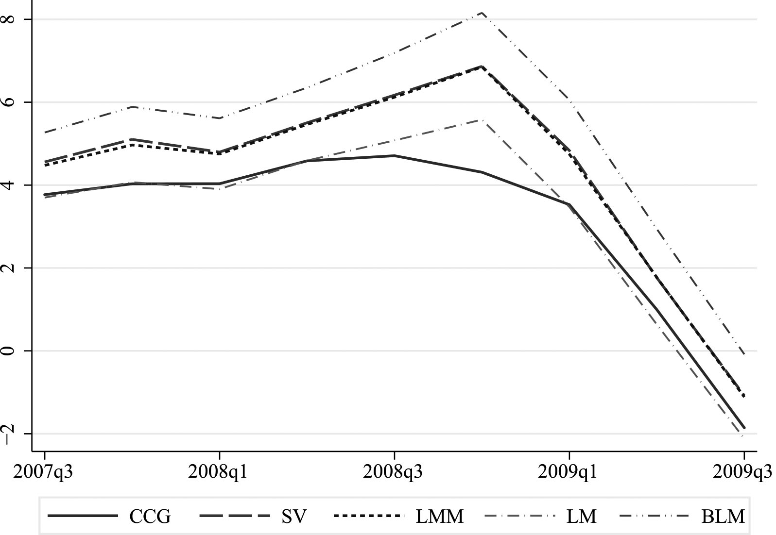

As discussed in Sections 3 and 4, these indexes are derived from the same CES model with time-varying taste parameters. Comparisons among $P_{\textit{LM}}$ , $P_{\textit{BLM}}$ , $P_{\textit{LMM}}$ , and $P_{\textit{SV}}$ shed light on the degree to which the estimate of pure price change is affected by the choice of conditioning taste vector. A difference such as $P_{\textit{CCV}}-P_{\textit{SV}}$ estimates the partial effect of tastes on the unconditional COLI (like in Eq. (7)), provided one treats utility as cardinal.

Table 7

Distribution of average CES index differences across product groups (percentage points)

	SV – CCV	SV – LMM	SV – BLM	BLM – LM
P5	$-$ 1.3823	$-$ 0.0892	$-$ 3.0150	0.2529
P10	$-$ 0.9184	$-$ 0.0587	$-$ 2.8766	0.3458
P25	0.0982	$-$ 0.0126	$-$ 1.0537	0.7227
P50	1.0619	0.0084	$-$ 0.7340	1.3341
P75	2.1459	0.0506	$-$ 0.3727	2.1260
P90	3.2087	0.1645	$-$ 0.1908	5.6108
P95	4.2060	0.1993	$-$ 0.1652	6.3208
Mean	1.1215	0.0516	$-$ 0.9869	2.0527

Notes: Based on data provided by The Nielsen Company (U.S.), LLC. Product group-level index differences are first averaged over time. Department and overall statistics are calculated using the product group’s share of average quarterly expenditure as weights. CCV refers to RW’s CES Common Varieties Index, SV refers to Sato-Vartia, LM refers to Lloyd-Moulton, BLM refers to Backwards Lloyd-Moulton, and LMM refers to the geometric mean of LM and BLM.

Figure 2.

Scantrak CES Price Index Averages By Dept. (% change versus year ago). Note: Based on data provided by The Nielsen Company (U.S.), LLC. See notes for Fig. 1.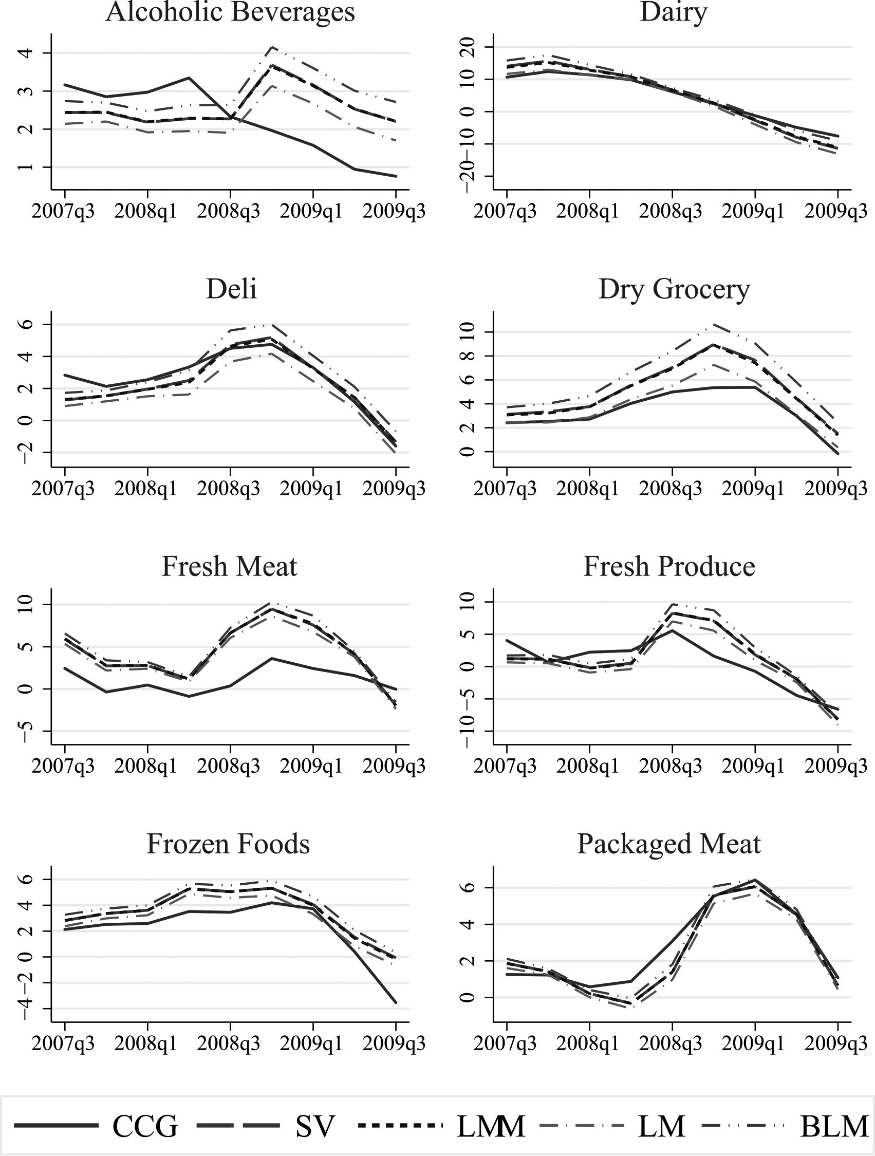

The Scantrack data show that, as in RW, the contributions of tastes tend to lower $P_{\textit{CCV}}$ relative to all of the conditional COLI save $P_{\textit{LM}}$ , which implies similar inflation. From Fig. 1, the unconditional and conditional COLI estimates tend to agree in sign, and accelerate and decelerate in similar patterns. $P_{\textit{CCV}}$ implies an average four-quarter percent change in the unconditional cost-of-living of 3.05 percentage points per year. Similar to RW, I find $P_{\textit{CCV}}$ tends to imply substantially lower inflation than $P_{\textit{SV}}$ . I find an average difference of 1.12 percentage points, while RW report an average of 0.4 percentage points. The difference may be due to the time periods covered (RW cover 2005 to 2013), the precise CGR (RW require items be present for at least six years), or the dataset used (RW use the Homescan consumer panel). Also using Scantrack data, but over the period 2006–2014, Figure 11 of Ehrlich et al. [15] finds taste-shock biases (also called consumer valuation bias) of 1 percentage point per year or greater depending on the CGR. While Fig. 1 suggests $P_{\textit{CCV}}$ tends to be much lower than most of the other conditional COLI estimates, Fig. 2 and Table 8 suggest considerable heterogeneity by department. The average $P_{\textit{SV}}-P_{\textit{CCV}}$ spread ranges from $-$ 0.36 percentage points for Packaged Meat to 3.20 percentage points for Fresh Meat. For Dry Grocery, Fresh Meat, and Frozen Foods, $P_{\textit{CCV}}$ fairly consistently implies lower inflation over time than $P_{\textit{SV}}$ , but for Alcohol, Dairy, Deli, Fresh Produce, and Packaged Meat, the sign of the gap is not consistent.

Table 8

Mean CES index differences, 2007Q3 – 2009Q3 (percentage points)

	SV – CCV	SV – LMM	SV – BLM	SV – LM	BLM – LM
Alcoholic Beverages	0.3701	0.0017	$-$ 0.3878	0.3895	0.7774
Dairy	0.0709	0.0103	$-$ 1.5332	1.5094	3.0427
Deli	$-$ 0.2684	0.0411	$-$ 0.6283	0.7058	1.3341
Dry Grocery	1.6768	0.0843	$-$ 1.1011	1.2399	2.3410
Fresh Meat	3.2006	$-$ 0.0343	$-$ 0.5956	0.5237	1.1193
Fresh Produce	0.5666	0.0118	$-$ 0.8645	0.8795	1.7441
Frozen Foods	1.3419	0.0294	$-$ 0.4684	0.5227	0.9911
Packaged Meat	$-$ 0.3586	$-$ 0.0011	$-$ 0.2966	0.2936	0.5902
All	1.1215	0.0516	$-$ 0.9869	1.0659	2.0527

Notes: Based on data provided by The Nielsen Company (U.S.), LLC. Product group-level index differences are first averaged over time. Department and overall averages are calculated using the product group’s share of average quarterly expenditure as weights. CCV refers to RW’s CES Common Varieties Index, SV refers to Sato-Vartia, LM refers to Lloyd-Moulton, BLM refers to Backwards Lloyd-Moulton, and LMM refers to the geometric mean of LM and BLM.

Turning to the conditional COLIs, the Scantrack estimates indicate that the choice of taste vector also impacts the measurement of price change. From Table 7, $P_{\textit{BLM}}$ exceeds $P_{\textit{LM}}$ by 2.05 percentage points on average and by 1.33 percentage points at the median. Looking across departments (Table 8), the average difference ranges from 0.59 for Packaged Meat, to 3.04 for Dairy. As Figs 1 and 2 illustrate, the average $P_{\textit{BLM}}-P_{\textit{LM}}$ gap is persistent and fairly stable over time. Conditioning on an intermediate level of tastes, $P_{\textit{SV}}$ in most cases is very close to $P_{\textit{LMM}}$ , the geometric average of reference-taste and comparison-taste indexes. Overall, they differ by 0.05 percentage points on average, and 0.008 percentage points at median, with average differences by all department less than 0.1 percentage points in magnitude. Conditioning on current preferences (as Fisher and Shell [19] prefer), $P_{\textit{BLM}}$ implies that consumers during this time period needed to increase expenditure by 5.15% on average to be indifferent between current and year-ago food and beverage prices. This is 0.99 percentage points greater than if measured using intermediate tastes ( $P_{\textit{SV}}$ ).

Figure 3.

CES Price Indexes: CGR versus All Matched UPCs (% change versus year ago). Note: Based on data provided by The Nielsen Company (U.S.), LLC. Plots are comparison expenditure-weighted averages of the four-quarter proportional changes implied by product group-level indexes for food and beverage products. CCV refers to RW’s CES Common Varieties Index, SV refers to Sato-Vartia, LM refers to Lloyd-Moulton, BLM refers to Backwards Lloyd-Moulton, and LMM refers to the geometric mean of LM and BLM. All but the SV indexes require estimated elasticities of substitution. An “A” in the label indicates all matched UPCs were included. Otherwise, the indexes cover only UPCs satisfying the CGR.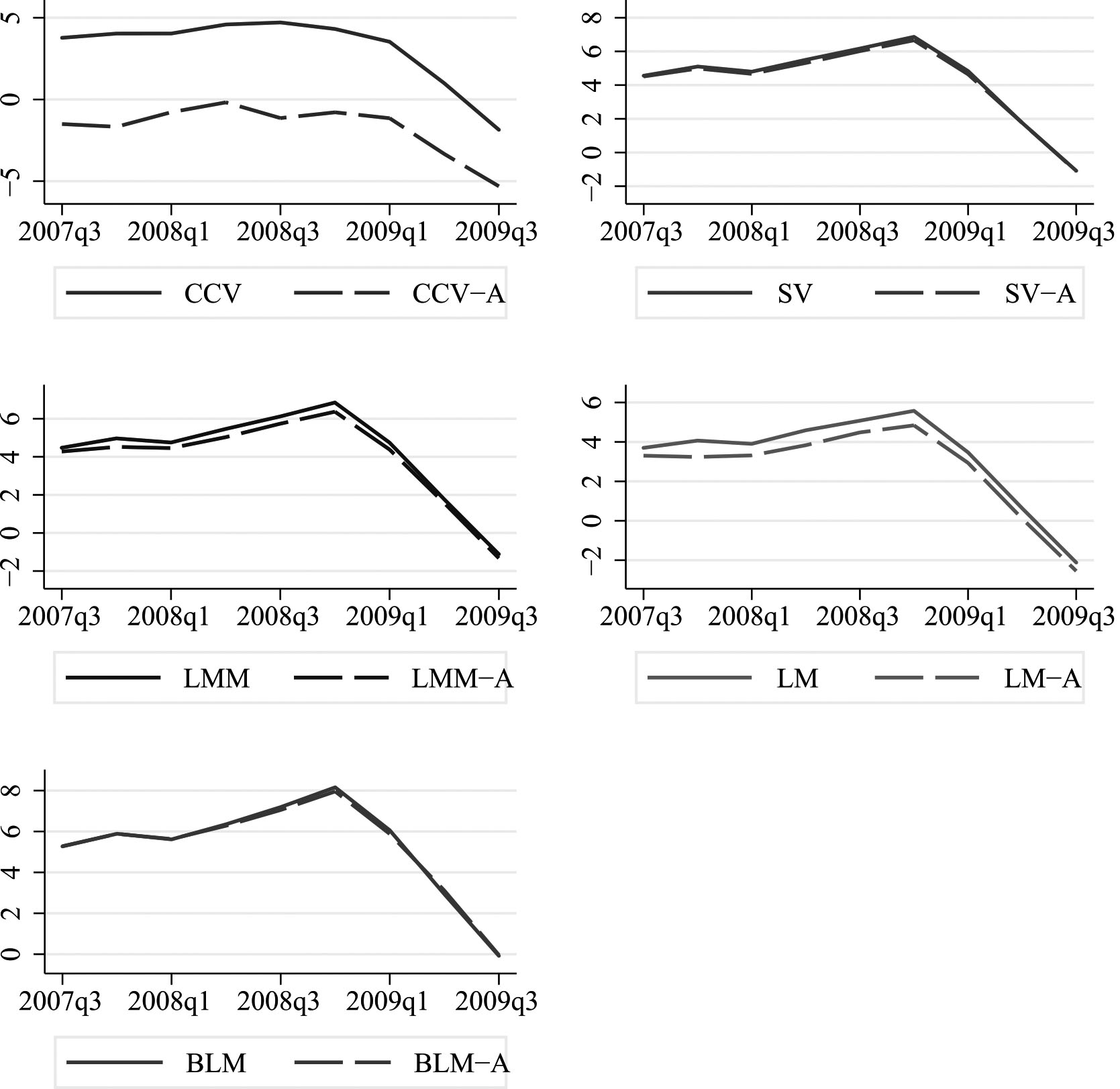

The results discussed thus far are based on a CGR intended to match RW’s as closely as possible. Now, I evaluate the impact of the CGR on the various index formulas by re-estimating the indexes using all UPCs that could be matched between quarters $t$ and $t-4$ . Figure 3 plots versions of each index – one using the CGR, and another (marked with an “A”) using all matched UPCs. The impact of extreme share changes on $P_{\textit{CCV}}$ is large. Without the CGR, the average inflation implied by $P_{\textit{CCV}}$ is 4.86 percentage points lower, implying deflation in most periods. Ehrlich et al. [15] also find that $P_{\textit{CCV}}$ is sensitive to the CGR. Table 9 and Fig. 3 also show the effect of the common goods definition on the CES conditional COLIs is smaller and would not change the sign of the index in most cases, amounting to only 0.11 percentage points on average for $P_{\textit{SV}}$ and 0.04 percentage points on average for $P_{\textit{BLM}}$ . The average impact on $P_{\textit{LM}}$ (and hence $P_{\textit{LMM}}$ ) is a bit larger (0.59 percentage points in magnitude). The fact that $P_{\textit{BLM}}$ is virtually unchanged, while $P_{\textit{LM}}$ is higher under the CGR perhaps implies that items on clearance (experiencing large price and share declines) have a greater impact than new entrants experiencing large share increases.

Table 9

Average CES Index by common goods definitions, 2007Q3 – 2009Q3 (perc. points)

	With CGR	Matched UPCs	Diff.
CCV	3.0468	$-$ 1.8178	4.8646
SV	4.1683	4.0539	0.1143
LMM	4.1167	3.7908	0.3258
LM	3.1024	2.5168	0.5856
BLM	5.1551	5.1192	0.0359

Notes: Based on data provided by The Nielsen Company (U.S.), LLC. Product group-level indexes are first averaged over time. Overall averages are then calculated using the product group’s share of average quarterly expenditure as weights. CCV refers to RW’s CES Common Varieties Index, SV refers to Sato-Vartia, LM refers to Lloyd-Moulton, BLM refers to Backwards Lloyd-Moulton, and LMM refers to the geometric mean of LM and BLM.

The descriptions of conditional and unconditional COLI presented in this section are based on a relatively simple model. Functional form may matter when estimating either the impact of tastes on a conditional COLI (e.g., $P_{\textit{BLM}}-P_{\textit{LM}}$ ) or the pure taste effect on the unconditional COLI, $P_{\textit{CCV}}-P_{\textit{SV}}$ . The reason is $P_{\textit{CCV}}$ , $P_{\textit{LM}}$ , and $P_{\textit{BLM}}$ can be written as recovering the taste parameters as residuals in the CES expenditure share equation. Martin [32] uses a simulation study that suggests a neglected nesting structure causes negative biases in $P_{\textit{CCV}}$ and $P_{\textit{LM}}$ , positive bias in $P_{\textit{BLM}}$ , and negligible bias in $P_{\textit{SV}}$ . The indexes tend to have the same rankings relative to each other, but index differences $P_{\textit{CCV}}-P_{\textit{SV}}$ and $P_{\textit{BLM}}-P_{\textit{LM}}$ can be overestimated. Quantification of taste changes, therefore, may be sensitive to model fit. However, as discussed in Section 3, COLI estimates based on intermediate tastes (or an average of COLI like LMM) may be robust to specification errors (provided $\sigma$ is not too large) because they fall in the class of superlative and quasi-superlative indexes [35]. Appendix A.1 compares traditional indexes using the Scantrack data. Similarity between the Sato-Vartia and the Fisher and Tornqvist (which approximate an arbitrary expenditure function) implies the CES assumption is not restrictive for estimating a COLI that conditions on average tastes.

6. Conclusion

In a model with changing preferences, there is no longer one true COLI, so it is important to carefully consider the intended theoretical targets when comparing alternative price indexes. When tastes change, the Tornqvist, Sato-Vartia, Lloyd-Moulton and CCV indexes all correspond to different true COLIs. These differ in whether they are intended to reflect only price change (and if so, what preference relation is referenced), or are intended to also capture the pure effect of changing tastes. Users should bear in mind that conditional COLIs are based on reaching a constant indifference curve, while an unconditional COLI is based on reaching a constant utility level. The latter is measurable only under a very strong assumption about utility. This paper’s empirical analysis suggests the set of common goods has a significant impact on the unconditional COLI. If all matched items are incorporated, the relative contribution of prices can be swamped by taste change effects. If there is interest in a COLI that conditions on a specific period’s taste vector, then this paper provides a novel empirical comparison for the CES case. Improvements to the simple CES model are likely possible, and so future research should include more general demand models to more precisely separate taste changes from price-related substitutions.

Footnotes

CE and PCE cover slightly different target populations and rely on different survey methods. See Passero et al. [] for a discussion.

Acknowledgments

I am grateful to Brian Adams, Rob Feenstra, Thesia Garner, Greg Kurtzon, and others for helpful comments. This paper uses data from The Nielsen Company (U.S.), LLC. All estimates, analysis, and errors are my own.

A. Appendix

References

National Research Council. At What Price: Conceptualizing and Measuring Cost-of-Living and Price Indexes. Schultze

and Mackie

. National Academies Press, 2002.

ILO. Consumer Price Index Manual: Theory and Practice. Ed. Hill P. Jointly published by ILO, IMF, OECD, UNECE, Eurostat, and the World Bank. 2004.

Caves

Christensen

Diewert

. The economic theory of index numbers and the measurement of input, output, and productivity. Econometrica: Journal of the Econometric Society. 1982; 1393-1414.

Redding

Weinstein

. Measuring aggregate price indices with taste shocks: Theory and evidence for CES Preferences. The Quarterly Journal of Economics. 2020; 135(1): 503-560. doi: 10.1093/qje/qjz031.

Klick

. Improving initial estimates of the Chained Consumer Price Index. Monthly Labor Review. 2018; 141. doi: 10.21916/mlr.2018.6.

Lloyd

. Substitution effects and biases in nontrue price indices. The American Economic Review. 1975; 65(3): 301-313.

Moulton

. Constant Elasticity Cost-of-Living Index in Share Relative Form. Tech. Rep. Bureau of Labor Statistics, 1996.

Hottman

Monarch

. A matter of taste: Estimating import price in ation across US income groups. Journal of International Economics. 2020; 127: 103382. doi: 10.1016/j.jinteco.2020.103382.

Ueda

Watanabe

. Product turnover and the cost of living index: quality vs. fashion effects. American Economic Journal: Macroeconomics. 2019; 11: 310-347. doi: 10.1257/mac.20160403.

10.

Phlips

Sanz-Ferrer

. A taste-dependent true index of the cost of living. The Review of Economics and Statistics. 1975; 495-501.

11.

Heien

Dunn

. The true cost-of-living index with changing preferences. Journal of Business & Economic Statistics. 1985; 3(4): 332-335.

12.

Sato

. The ideal log-change index number. The Review of Economics and Statistics. 1976; 223-228.

13.

Vartia

. Ideal log-change index numbers. Scandinavian Journal of Statistics. 1976; 121-126.

14.

Balk

. Changing consumer preferences and the cost-of-living index: Theory and nonparametric expressions. Journal of Economics. 1989; 50(2): 157-169.

15.

Ehrlich

et al. Quality adjustment at scale: Hedonic vs. Exact demand-based price indices. Paper prepared for the 36th IARIW Virtual General Conference. 2021.

16.

Konüss

. The problem of the true index of the cost of living. Econometrica. 1939; 7: 10-29.

17.

Cage

Greenlees

Jackman

. Introducing the chained consumer price index. In: International Working Group on Price Indices (Ottawa Group): Proceedings of the Seventh Meeting. Paris: INSEE. 2003; pp. 213-246.

18.

Diewert

. Exact and superlative index numbers. Journal of Econometrics. 1976; 4(2): 115-145.

19.

Fisher

Shell

. Taste and quality change in the pure theory of the true cost-of-living index. The Economic Theory of Price Indices. Academic Press. 1972; pp. 1-48.

20.

Muellbauer

. The cost of living and taste and quality change. Journal of Economic Theory. 1975; 10(3): 269-283.

21.

Kurtzon

. The problem with normalizing preferences that change in a cost-of-living index. BLS Working Paper. 2020; p. 534. https//www.bls.gov/osmr/research-papers/2020/pdf/ec200160.pdf.

22.

Feenstra

. New product varieties and the measurement of international prices. American Economic Review. 1994; pp. 157-177.

23.

Gábor-Tóth

Vermeulen

. The relative importance of taste shocks and price movements in the variation of cost-of-living: Evidence from scanner data. Unpublished Working Paper available at SSRN. 2018; 3246221.

24.

Diewert

. The consumer price index and index number purpose. Journal of Economic and Social Measurement. 2001; 27(3,4): 167-248. doi: 10.3233/JEM-2003-0183.

25.

Feenstra

Reinsdorf

. Should exact index numbers have standard errors? Theory and application to asian growth. In: Hard-to-Measure Goods and Services: Essays in Honor of Zvi Griliches. University of Chicago Press, 2007; pp. 483-513.

26.

Balk

. On curing the CPI’s substitution and new goods bias. Presented at the Fifth Meeting of the International Working Group on Price Indices, Reykjavik, 25-27 August 1999.

27.

Melser

. Accounting for the effects of new and disappearing goods using scanner data. Review of Income and Wealth. 2006; 52(4): 547-568. doi: 10.1111/j.1475-4991.2006.00203.x.

28.

Pakes

. A Reconsideration of Hedonic Price Indexes with an Application to PC’s. American Economic Review. 2003; 93(5): 1578-1596. doi: 10.1257/000282803322655455.

29.

Nevo

. New products, quality changes, and welfare measures computed from estimated demand systems. Review of Economics and Statistics. 2003; 85(2): 266-275. doi: 10.1162/003465303765299792.

30.

Mas-Colell

Whinston

Green

, et al. Microeconomic theory. Vol. 1. Oxford University press New York, 1995.

31.

Pollak

. The Theory of the Cost-of-Living Index. Oxford University Press on Demand, 1989.

32.

Martin

. Taste change versus specification error in cost-of-living measurement. BLS Working Paper. 2020; 531. https//www.bls.gov/osmr/research-papers/2020/pdf/ec200130.pdf.

33.

Fisher

. The Making of Index Numbers: A Study of Their Varieties, Tests, and Reliability. Houghton Mifflin, 1922.

34.

de Haan

Balk

Hansen

. Retrospective approximations of superlative price indexes for years where expenditure data is unavailable. Price Indexes in Time and Space. Springer. 2010; pp. 25-42. doi: 10.1007/978-3-7908-2140-6_2.

35.

Diewert

. Superlative index numbers and consistency in aggregation. Econometrica. 1978; 46(4): 883-900.

36.

Hill

. Superlative index numbers: not all of them are super. Journal of Econometrics. 2006; 130(1): 25-43. doi: 10.1016/j.jeconom.2004.08.018.

37.

Deaton

Muellbauer

. Economics and Consumer Behavior. Cambridge University Press, 1980.

38.

StataCorp. Stata/SE Version 151. for Windows (64-bit, x86-64), Revision 15 Oct 2018. Oct. 15, 2018. https//www.stata.com.

39.

Broda

Weinstein

. Product creation and destruction: evidence and price implications. American Economic Review. 2010; 100: 691-723. doi: 10.1257/aer.100.3.691.

40.

Bureau of Labor Statistics. Average annual expenditures and characteristics of all consumer units, Consumer Expenditure Survey, 2006–2012. Tech. Rep. 2019; https//www.bls.gov/cex/2012/standard/multiyr.pdf.

41.

Bureau of Economic Analysis. 2019; https//www.bea.gov.

42.

Ehrlich

et al. Re-engineering Key National Economic Indicators. In: Big Data for 21st Century Economic Statistics. University of Chicago Press, 2019.

43.

Passero

Garner

McCully

. Understanding the Relationship: CE Survey and PCE. In: Improving the Measurement of Consumer Expenditures. University of Chicago Press. 2014; pp. 181-203.

44.

Hansen

. Large sample properties of generalized method of moments estimators. Econometrica: Journal of the Econometric Society. 1982; pp. 1029-1054.

45.

Broda

Weinstein

. Globalization and the gains from variety. The Quarterly Journal of Economics. 2006; 121(2): 541-585. doi: 10.1162/qjec.2006.121.2.541.

46.

Bureau of Labor Statistics. 2020. https//www.bls.gov/cpi/tables/relative-importance/2019.txt.

47.

Bureau of Labor Statistics. Chapter 17. The Consumer Price Index. In: Handbook of Methods. Bureau of Labor Statistics, 2018.

48.

Abe

Rao

. Generalized logarithmic index numbers with demand shocks-bridging the gap between theory and practice. RCESR Discussion Paper DP20-1. 2020.

49.

Redding

Weinstein

. Measuring aggregate price indexes with demand shocks: theory and evidence for CES preferences. NBER Working Paper 22479 (Accessed 6/4/2018). May 2018.

Revisiting taste change in cost-of-living measurement

Abstract

Keywords

1. Introduction

2. Existing literature

3. Cost-of-living theory

3.1 Conditional COLI

.

.

.

.

.

.

.

.

5. Application to retail scanner data

5.1 Data and model estimation

Table 2 Scantrack food and beverage departments

Footnotes

Acknowledgments

A. Appendix

References

Table 2
Scantrack food and beverage departments