Standardizing the CAP Score in Huntington’s Disease by Predicting Age-at-Onset

Abstract

Background:

Huntington’s disease (HD) is an autosomal dominant, neurological disease caused by an expanded CAG repeat near the N-terminus of the huntingtin (HTT) gene. A leading theory concerning the etiology of HD is that both onset and progression are driven by cumulative exposure to the effects of mutant (or CAG expanded) huntingtin (mHTT). The CAG-Age-Product (CAP) score (i.e., the product of excess CAG length and age) is a commonly used measure of this cumulative exposure. CAP score has been widely used as a predictor of a variety of disease state variables in HD. The utility of the CAP score has been somewhat diminished, however, by a lack of agreement on its precise definition. The most commonly used forms of the CAP score are highly correlated so that, for purposes of prediction, it makes little difference which is used. However, reported values of CAP scores, based on commonly used definitions, differ substantially in magnitude when applied to the same data. This complicates the process of inter-study comparison.

Objective:

In this paper, we propose a standardized definition for the CAP score which will resolve this difficulty. Our standardization is chosen so that CAP = 100 at the expected age of diagnosis.

Methods:

Statistical methods include novel survival analysis methodology applied to the 13 disease landmarks taken from the Enroll-HD database (PDS 5) and comparisons with the existing, gold standard, onset model.

Results:

Useful by-products of our work include up-to-date, age-at-onset (AO) results and a refined AO model suitable for use in other contexts, a discussion of several useful properties of the CAP score that have not previously been noted in the literature and the introduction of the concept of a toxicity onset model.

Conclusion:

We suggest that taking L = 30 and K = 6.49 provides a useful standardization of the CAP score, suitable for use in the routine modeling of clinical data in HD.

Keywords

Huntington’s disease CAP Score age-at-onset time-to-event models

INTRODUCTION

Huntington’s disease (HD) is an autosomal dominant, neurological disease caused by an expanded CAG repeat near the N-terminus of the huntingtin (HTT) gene on chromosome 4. A leading theory concerning the etiology of HD is that both onset and progression are driven by cumulative exposure to the effects of mutant (or CAG expanded) huntingtin (mHTT) via the huntingtin protein (whole or toxic fragments) or RNA [1 –4]. The CAP score (CAG-Age-Product, i.e., the product of excess CAG length and age) is a commonly used measure of this cumulative exposure that has been widely used as a predictor of a variety of disease state variables in HD including imaging (structural MRI [5, 6] diffusion tensor imaging [6, 7] and PDE10A PET imaging [8]), various empirical measures of HD signs and symptoms [9], wet biomarkers (neurofilament light [10]), the onset of motor symptoms [11], and disease stage [12].

As defined in [9] CAP has the following general form $CAP = AGE \times {(CAG - L)}_{+} / K$ (1) where L and K are constants and (x)₊ is a function that equals x, when x≥0 and 0 otherwise. Here L is an estimate of the lower limit of CAG expansion values for which toxicity occurs and K standardizes the CAP score so that it is equal to 100 at the expected age of onset. People who have CAG lengths > 35 are known as HD gene expansion carriers (HDGECs). The disease is said to be fully penetrant when CAG≥40.

Since mHTT is present from conception in HDGECs, the CAP score can be thought of as the product of a measure of a toxic insult (excess CAG length) with the time over which the toxic insult is exercised (given approximately by age). In this respect CAP score is similar to the pack-years measure used in the study of the toxic effects of tobacco or the area under the curve (AUC) measure used in PK/PD analysis and toxicology. This equivalence assumes that CAG length is constant from conception, an assumption that is made in all analyses presented below. It is now known, however, that CAG length is unstable and tends to expand somatically, in a tissue-dependent manner [13], particularly in the striatum, a brain region where the most pronounced pathology is observed. CAG, as it appears in Equation 1, is measured (as is routinely done) in white blood cells which are believed, on the whole, to retain their original baseline values from conception. Reliable measurements of CAG length in living human brains is not currently available and, as a result, the practical significance of somatic expansion and the degree to which somatic expansion is reflected in the CAP score, remain unclear. We will return to these matters of interpretation in the discussion.

The utility of the CAP score has been somewhat diminished by a lack of agreement on the values of L and K across studies. The most common values for L that appear in the literature are L = 33.66 [11 , 15]; L = 35.5 [16, 17]; and L = 30 [5, 9]. K has received less attention. Two papers have linked K with the expected age at motor onset [5, 9] such that CAP = 100 at this age. This linkage was carried out via a simple time-to-event model which models the time between birth and onset (i.e., age-at-onset, AO). A similar time-to-event model and value of K was presented in [11] but the starting time for this model was entry into the Predict-HD study [18] and K was chosen so that CAP = 1 when there is a 50% chance of a diagnosis in the next 5 years. More commonly the use of CAP with L = 33.66 or L = 35.5 is combined with K = 1 leaving the connection with AO undefined. The value of 35.5 is not supported by any model for AO but it coincides with the lower limit of CAG length at which HD diagnosis has been confirmed (36 repeats). CAP scores with all the above values of L and K are highly correlated (Table 1) so, for purposes of prediction, it makes little difference which is used. However, [19] reported values of CAP scores, computed on the same data, differ substantially when different values of L and K are used and CAP scores based on differing values of L, when evaluated at the age of onset, have substantially different correlations with CAG length. Finally, the relationship between summary statistics (i.e., means and standard deviations) based on CAP scores that are computed using differing values of L and K is dependent on the distribution of ages and CAG lengths in each study. All of this complicates the process of inter-study comparison. Standardization is clearly needed.

Table 1

Correlations of CAP Scores for L = 27 to 35.5

	cap27	cap28	cap29	cap30	cap32	cap33.66	cap35.5
cap27	1.000	0.999	0.995	0.988	0.955	0.900	0.793
cap28	0.999	1.000	0.999	0.994	0.968	0.919	0.820
cap29	0.995	0.999	1.000	0.998	0.979	0.938	0.849
cap30	0.988	0.994	0.998	1.000	0.990	0.957	0.878
cap32	0.955	0.968	0.979	0.990	1.000	0.989	0.938
cap33.66	0.900	0.919	0.938	0.957	0.989	1.000	0.979
cap35.5	0.793	0.820	0.849	0.878	0.938	0.979	1.000

In this paper, we propose that L = 30 and K = 6.49 be the preferred values for these parameters in HD research, unless special circumstances dictate otherwise, or a more physiologically based model becomes available. As we show below, the justification for this choice is that these values ensure that CAP 100 at the expected age of onset (under a reasonable definition of onset and a reasonable onset model). In addition, the use of this choice of L and K greatly reduces the correlation of CAP scores, evaluated at the age of onset, with CAG lengths. The most common use of the CAP score is in the prediction of continuous disease state variables in natural history studies which raises the concern that use of CAP scores with values of L substantially different from 30 may induce spurious correlations with CAG length.

To justify the above choice for L and K, we

Define a novel AO model that extends previous well-accepted models

Use this model to compute values of L and K that cause CAP ∼100 at the expected age-at-onset

Validate the new model by showing that it produces AO results that are:

comparable to those of the current gold standard AO model [19]

closely matched by non-parametric survival plots of CAP scores

in good agreement with models optimized to fit each specific onset measure in Table 2.

Table 2

Definitions of onset variables

1	hddiagn	Age of HD clinical diagnosis
2	sxrater	Rater’s estimate of age of symptom onset
3	sxsubj	Age at which symptoms were first noted by participant
4	sxfam	Age at which symptoms were first noted by participant’s family
5	ccmtrage	At what age did the participant’s motor symptoms begin?
6	cccogage	At what age did cognitive impairment first start to have animpact on daily life?
7	ccdepage	At what age did depression begin?
8	ccirbage	At what age did irritability begin?
9	ccvabage	At what age did violent or aggressive behavior begin?
10	ccaptage	At what age did apathy begin?
11	ccpobage	At what age did perseverative obsessive behavior begin?
12	ccpsyage	At what age did psychosis (hallucinations or delusions) begin?
13	DCL4	Age of first occurrence of Diagnostic Confidence Level (DCL)=4

A non-parametric method for deriving the optimal value of L is also presented.

Useful biproducts of the above program are

Up-to-date AO results for the publicly available periodic dataset (PDS5, Oct 31, 2020) release from Enroll-HD

A refined AO model suitable for use in other contexts

A discussion of several useful properties of the CAP score that have not previously been noted in the literature: these include an alternative parameterization of CAP and a demonstration that, properly defined, CAP at onset is independent of CAG length

The introduction of the concept of a toxicity onset model.

METHODS AND MATERIALS

Data

All models were fit to data from the PDS 5 release of the Enroll-HD database [20, 21]. Separate analyses for a total of 13 AO variables are presented. The first 12 AO variables appear in the Enroll data set in the Profile data file and reflect retrospective assessments of time of onset from the rater, the participant, and the participant’s family. The final variable DCL4 is defined prospectively in terms of the diagnostic confidence level (diagconf = 4) from the UHDRS motor assessment. Unlike the first 12 variables, DCL4 will always be left censored for participants that enter Enroll in the manifest state. That is, for participants that enter Enroll with diagconf = 4, age-at-onset according to DCL4 is known only to be less than or equal to age-at-study-entry. All 13 variables are defined in Table 2. The primary variable, hddiagn, provides the age of the participant’s medical diagnosis for HD. Like all of the first 12 onset variables, hddiagn differs from DCL4 in that it reflects retrospectively collected information on participants that enter the study in a manifest state. In this respect, the first 12 onset variables are similar to age-at-onset as defined in [19]. A second variable, sxrater, closely related to hddiagn, encodes the rater’s best estimate of the time of first occurrence of HD symptoms. Rater’s are trained but are not necessarily medical professionals. Thus sxrater and hddiagn target different landmarks in the course of the disease. Except for a few rare anomalies, hddiagn will be later than sxrater, particularly if the participant makes infrequent visits to the physician or if, at a given visit, the physician feels that it is in the best interest of the participant to delay a formal diagnosis. The variables sxsubj and sxfam provide retrospective assessments of the participant and the participant’s family as to the first occurrence of any symptom of HD. Variables ccmtrage, cccogage, ccdepage, ccirbage, ccvabage, ccaptage, ccpobage, and ccpsyage record the rater’s assessment of the first time that various symptoms were noted. Symptoms include (in order) motor, cognitive, depression, irritability, violent or aggressive behavior, apathy, perseverative obsessive behavior, and psychosis. See Table 2 for complete definitions of these symptoms. Only the motor symptoms are defined in relation to HD. In all other cases the rater is asked to record the first time that the symptom occurred without reference to the cause.

Following [19] our analysis considered only HDGECs with CAG lengths between 40 and 56 (inclusive) and ages at entry into the Enroll study between 20 and 80 (inclusive). Event times for each of the variables in Table 2 are classified as “Uncensored” (time of event recorded), “Right Censored” (event has not yet occurred at time of last observation) and “Left Censored” (event only known to have occurred prior to the time of last observation) or “Unclassifiable”. Unclassifiable events were dropped from the analysis as were cases with very early onset to be described in the Supplementary Material. Table 3 tabulates the censoring data for each variable. Internal Enroll documents show that study retention is high, particularly among pre-manifest participants (80% over 7 years) so that right censoring is mostly determined by the age of the subject at entry. Left censoring is mostly determined by the ability of participants or their caregivers to recall onset times or by the quality of medical records. Given all of this, we chose to treat censoring as uninformative.

Table 3

Censoring status by onset variable

	Variable	Uncensored	Right censored	Left censored	Dropped (unclassifiable)	Dropped (early AO)¹
1	hddiagn	10634	4033	0	258	6
2	sxrater	10272	3933	698	0	28
3	sxsubj	10596	3659	169	451	56
4	sxfam	10196	3680	160	835	60
5	ccmtrage	11276	3492	132	9	22
6	cccogage	6480	8218	192	11	30
7	ccdepage	9582	4783	161	8	397
8	ccirbage	8822	5629	214	13	253
9	ccvabage	4965	9676	130	13	147
10	ccaptage	7848	6794	186	13	90
11	ccpobage	6715	7802	238	17	159
12	ccpsyage	1527	13332	46	8	18
13	DCL4	1171	4135	9625	0	0

¹See supplementary material.

CAP score onset models

The CAP score onset models used here are instances of a general class of models (which we call toxicity onset models) that can be used whenever a toxic insult, suffered over time, is believed to cause the onset of an event. Suppose that we have a model for the time course of the toxic insult TOX(t, θ), where θ is a parameter to be estimated. We define $AUC (T, θ) = \int_{0}^{T} TOX (t, θ) dt$ (2)

The toxicity onset model assumes that the event occurs when AUC exceeds a random limit. In mathematical symbols $AUC (T, θ) = μ + ɛ$ (3) where T is a, possibly censored, event time, μ is an unknown value of the “fixed effect” part of the limit and ɛ is a mean zero random variable with scale parameter σ giving the “random effect” portion of the limit. Analysis proceeds by applying standard survival analysis methodology to the event time T. In particular, the distribution function F(T) is given by $F (T, θ, μ, σ) = Φ (\frac{AUC (T, θ) - μ}{σ})$ (4) where Φ is the distribution function of E. The density, hazard, and survivor functions of T can be derived in the usual way from Equation 4, as is done in [22, and described below under “Model fitting procedures”. Note that in cases where differentiation is required, it is carried out with respect to T, not AUC.

The CAP score onset model is a toxicity onset model with $TOX = CAG - L$ (5) $AUC = (CAG - L) T$ (6) and Φ is a modified logistic distribution as described below. A more complex example of a toxicity onset model is given in the Discussion.

The clock for the event time (T) starts at birth and stops when either an onset event or a censoring event takes place. Under the model, the cumulative probability of onset, as a function of CAP, has the following form. $\begin{matrix} F (x) \equiv Pr (CAP (T, CAG) < x) \\ = P \frac{exp (β_{0} (x - μ_{0}))}{1 + exp (β_{0} (x - μ_{0})}) \end{matrix}$ (7) where T is the age-of-onset or an appropriately chosen censoring time. Equation 7 expresses the imposed model under which CAP follows a logistic distribution with location μ₀ and scale parameter (σ₀ = 1/β₀). The parameter P to model situations in which not all subjects are expected to experience onset: this happens in several of the variables in Table 2 (most notably those involved in forms of “psychiatric” onset). CAP, in Equation 7, may be defined using two equivalent parameterizations. $CAP \equiv \frac{AGE \times (CAG - L)}{K}$ (8) $CAP = \frac{AGE \times (1 + α (CAG - CA G_{0}))}{K_{α}}$ (9)

The number CAG₀ in Equation 9 is a reference value (or centering constant). Model predictions are not affected by the choice of CAG₀ provided that this parameter is chosen to be reasonably close to the population mean of CAG values in the study population. In what follows we always take CAG₀ = 43.

The above parameterizations for CAP are equivalent if and only if $\begin{matrix} α = 1 / (CA G_{0} - L) \\ K_{α} = K / (CA G_{0} - L) . \end{matrix}$ (10)

By fixing the value of μ₀ at 100 in Equation 7, one can find values of L and K (or α and K_α) which force CAP to be equal to 100 at the expected age-at-onset a useful normalizing property. We retain the two definitions of CAP from Equations 8 and 9 because both have their advantages. In particular, the definition in Equation 8 captures the interpretation of CAP as a measure of cumulative toxicity. In contrast, the definition in Equation 9 produces models with parameters that are easier to distinguish (i.e., less highly correlated). More importantly, the special case where CAG length has no effect on AO, occurs when α= 0, L = –∞, making it very awkward to test the hypothesis of CAG independence using the parameterization of Equation 8.

Finally, we note that Equation 7 can be expressed directly in terms of the age-at-onset (as opposed to the CAP-score-at-onset, leading to an expression of the form $Pr (AGE - AT - ONSET < x) = P \frac{exp (\frac{x - μ}{σ})}{1 + exp (\frac{x - μ}{σ})}$ (11) where $μ = \frac{μ_{0}}{CAG - L},$ (12) $σ = \frac{σ_{0}}{CAG - L} .$ (13)

The parameterization using μ and σ is similar to that used in the model of [19] and is therefore useful when making comparisons with that model. The parameterization of Equation 11 is also useful in comparing models with differing values of L.

Four models (each based on Equation 7) were fit.

Model 1: μ fixed at 100

Model 2: μ₀ fixed at 100, α fixed at 1/13.

Model 3: K_α fixed at 6.49/13 (Individually Optimized CAP Score Model).

Model 4: α fixed at 1/13, K_α fixed at 6.49/13 (Standard CAP Score Model).

For purposes of estimation, all models are defined in terms of the parameterization of Equation 9. The parameters L and K are then calculated using Equation 10. We note that, when α and K_α are fixed by design, α= 1/13 implies L = 30 and K_α = 6.49/13 implies K = 6.49. Models 1 and 2 are only fit to the age-at-diagnosis variable (hddiagn) and are used to find a definition of CAP score that is 100 at the expected age of diagnosis. Models 3 and 4 are fit to all 13 onset variables. Model 3 allows the effect of CAG length to be modeled separately for each onset variable. In addition, Model 3 is used to test the hypothesis of CAG independence (α= 0). Model 4 represents the recommended standardization for CAP Score.

Model fitting procedures

All models were formulated using standard time-to-event methodology, e.g., [22]. In particular, an uncensored event contributes a factor of f(t₁) to the likelihood function, a right censored event contributes a factor of 1 –F(t₂) to the likelihood function, and a left censored event contributes a factor of F(t₃) to the likelihood function. Here F(x) is as defined in Equation 7; and t₁, t₂ and t₃ are uncensored, right censored and left censored event times (see Section 1 of the Supplementary Material for operational definitions of these event times). Note that derivatives are always taken with respect to time and censoring is always modeled on the time scale.

All parametric survival models were fit using the STAN Bayesian Analysis Software Package [23] accessed through the Rstan package [24]. Models were fit using both optimization (LBFGS algorithm) and Hamiltonian Monte Carlo (NUTS algorithm). All reported modeling results were based on the former algorithm except for the Bayesian confidence intervals that appear in the Supplementary Material, and results on posterior correlations, which were computed using the latter algorithm. When Hamiltonian Monte Carlo was used, four chains with 4000 iterations (1000 of which were warm-up) were generated. Model fits are compared with non-parametric estimates of the survival curves based on observed CAP scores. Non-parametric survival curves were estimated using the Survival package in R [25]. In particular, non-parametric survival plots were obtained by applying the Surv function with interval censoring using CAP score as the time variable: this function implements the algorithm of Turnbull [26]. Data analysis and graphics were done in R version 3.61 [27].

Demonstration that CAP(AO, CAG) is independent of CAG

Under our model, it might be supposed that the CAP score captures all of the effects of CAG length on disease progression. This is a very strong statement and, while plausible in our view, very hard to justify in general. A weaker (but still very strong) form of the above statement is that CAP evaluated at the age-of-onset has a distribution in the population of HDGECs that is independent of CAG length. We present evidence in favor of this latter statement by showing that non-parametric estimates of CAP at onset agree with estimates based on our logistic model whenever sample sizes are large enough to support accurate nonparametric analysis. In addition, we show that the constant L can be estimated with some precision by finding values of L such that CAP at onset is uncorrelated with CAG length. Finally, we present graphs of the correlation of CAP(L) with CAG against L: these may be helpful in assessing the models based on our standardized value of L = 30 versus models based on outcome specific values of L or other values of L that have appeared in the literature.

RESULTS

Determining L and K

Parameter estimates for the primary age-at-onset variable (hddiagn) for Model 1 appear in the first row of Table 4 and show that when μ₀ is forced to take on the value 100, the parameters L and α will take on the values 30.674 and (0.081. In light of this, it seemed reasonable to fix L at 30 for the standardized value of CAP and, applying Equation 10, α=1/13 = 0.077. The second row of Table 4 now gives a value of K = 6.594 and K_α = 0.507. The above value for K which is very close to 6.49 that was recommended in [28] and which, for reasons of historical continuity, we would like to retain. This is the basis for the recommendation of L = 30 and K = 6.49 (α= 1/13 and K_α = K/13). We note that the posterior correlation of K and L is –0.98 while the posterior correlation of K_α and α is 0.077: this justifies our use of the parameterization for CAP given in Equation 9 and also provides an explanation for the difference between the estimated parameter values given here and previously reported values and for the very modest changes that these shifts appear to have on model predictions.

Table 4

Parameter estimates: model 1 and model 2 for onset variable hddiagn

Model	p	μ₀	β₀	σ ₀	α	Kα	L	K
1	1.000	100	0.122	8.181	0.081	0.508	30.674	6.257
2	1.000	100	0.122	8.197	0.077	0.507	30.000	6.594

Parameter estimates in Table 6, correspond to Model 4 and reflect results that obtain if the standardized CAP score is used. Finally, Table 5 shows results based on Model 3 which represent fits that are optimal for each individual onset variable. The variability in values of K_α between Tables 4 –6 is due to the different parameter restrictions place on these models, as described above. Comparison of the log likelihood statistics between Model 3 and Model 4 appear in Table 7. These values are often statistically significant, sometimes markedly so. However, in light of the very large sample sizes in the current study, it is important to bear in mind that effects that are statistically significant may have little or no clinical significance. In the interest of providing a useful standardization of the CAP score, we adopt a policy of focusing primarily on clinical significance as defined in the graphical representations in Figs. 1–3, which describe variables hddiagn, sxrater, and ccdepag). These figures make use of the parameterization of Equation 11 to compare predictions from the individually optimized fits (Model 3) with the standard model (Model 4). The Supplementary Material (Section 3) provides plots for each of the onset events in Table 2. In many cases, the model fits are seen to be so close that a small random jitter had to be introduced in order to visually distinguish Model 3 and Model 4 results. In other cases, some deviations between Models 3 and 4 are apparent but, at least in our view, these are small.

Table 6

Parameter estimates: standard model (model 4) by onset variable

	Variable	p	μ₀	β₀	σ ₀	α	Kα	L	K
1	hddiagn	1.000	102	0.120	8.329	0.077	0.499	30.000	6.490
2	sxrater	1.000	95	0.116	8.609	0.077	0.499	30.000	6.490
3	sxsubj	1.000	97	0.104	9.574	0.077	0.499	30.000	6.490
4	sxfam	1.000	95	0.111	9.049	0.077	0.499	30.000	6.490
5	ccmtrage	1.000	96	0.121	8.262	0.077	0.499	30.000	6.490
6	cccogage	0.918	109	0.086	11.594	0.077	0.499	30.000	6.490
7	ccdepage	0.966	94	0.055	18.088	0.077	0.499	30.000	6.490
8	ccirbage	0.959	100	0.062	16.211	0.077	0.499	30.000	6.490
9	ccvabage	0.800	114	0.055	18.151	0.077	0.499	30.000	6.490
10	ccaptage	0.976	108	0.069	14.407	0.077	0.499	30.000	6.490
11	ccpobage	0.988	113	0.062	16.219	0.077	0.499	30.000	6.490
12	ccpsyage	0.449	130	0.058	17.374	0.077	0.499	30.000	6.490
13	DCL4	0.999	88	0.121	8.264	0.077	0.499	30.000	6.490

Table 5

Parameter estimates: individually optimized model (model 3) by onset variable

	Variable	p	μ₀	β₀	σ ₀	α	Kα	L	K
1	hddiagn	1.000	102	0.120	8.318	0.081	0.499	30.674	6.154
2	sxrater	1.000	95	0.116	8.586	0.084	0.499	31.028	5.977
3	sxsubj	1.000	97	0.104	9.586	0.081	0.499	30.685	6.148
4	sxfam	0.999	96	0.111	9.029	0.082	0.499	30.873	6.054
5	ccmtrage	1.000	96	0.121	8.244	0.082	0.499	30.846	6.068
6	cccogage	0.918	109	0.086	11.602	0.081	0.499	30.695	6.143
7	ccdepage	1.000	96	0.053	18.779	0.069	0.499	28.574	7.202
8	ccirbage	0.962	100	0.062	16.238	0.070	0.499	28.733	7.122
9	ccvabage	0.799	114	0.055	18.146	0.078	0.499	30.137	6.421
10	ccaptage	0.978	108	0.069	14.420	0.075	0.499	29.649	6.665
11	ccpobage	0.989	113	0.062	16.225	0.075	0.499	29.695	6.642
12	ccpsyage	0.451	130	0.058	17.371	0.075	0.499	29.701	6.639
13	DCL4	0.999	88	0.121	8.244	0.086	0.499	31.389	5.797

Table 7

Chi-square tests to compare the standard model (model 4) with the individually optimized model (model 3) by onset variable (df = 1)

	Variable	Δ log-lik	p
1	hddiagn	58.16	0.00
2	sxrater	120.16	0.00
3	sxsubj	37.39	0.00
4	sxfam	75.80	0.00
5	ccmtrage	90.41	0.00
6	cccogage	24.27	0.00
7	ccdepage	9.13	0.00
8	ccirbage	37.64	0.00
9	ccvabage	0.30	0.58
10	ccaptage	4.37	0.04
11	ccpobage	2.78	0.10
12	ccpsyage	0.59	0.44
13	DCL4	112.81	0.00

Fig. 1

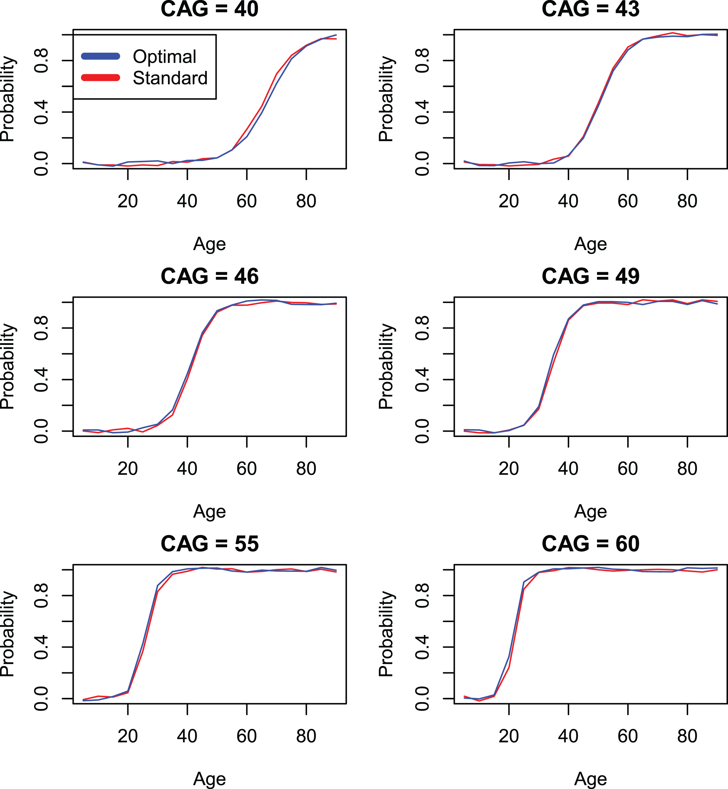
Comparison of standard CAP score models with individually optimized models (models 4 and 3) by onset variable hddiagn.

Fig. 2

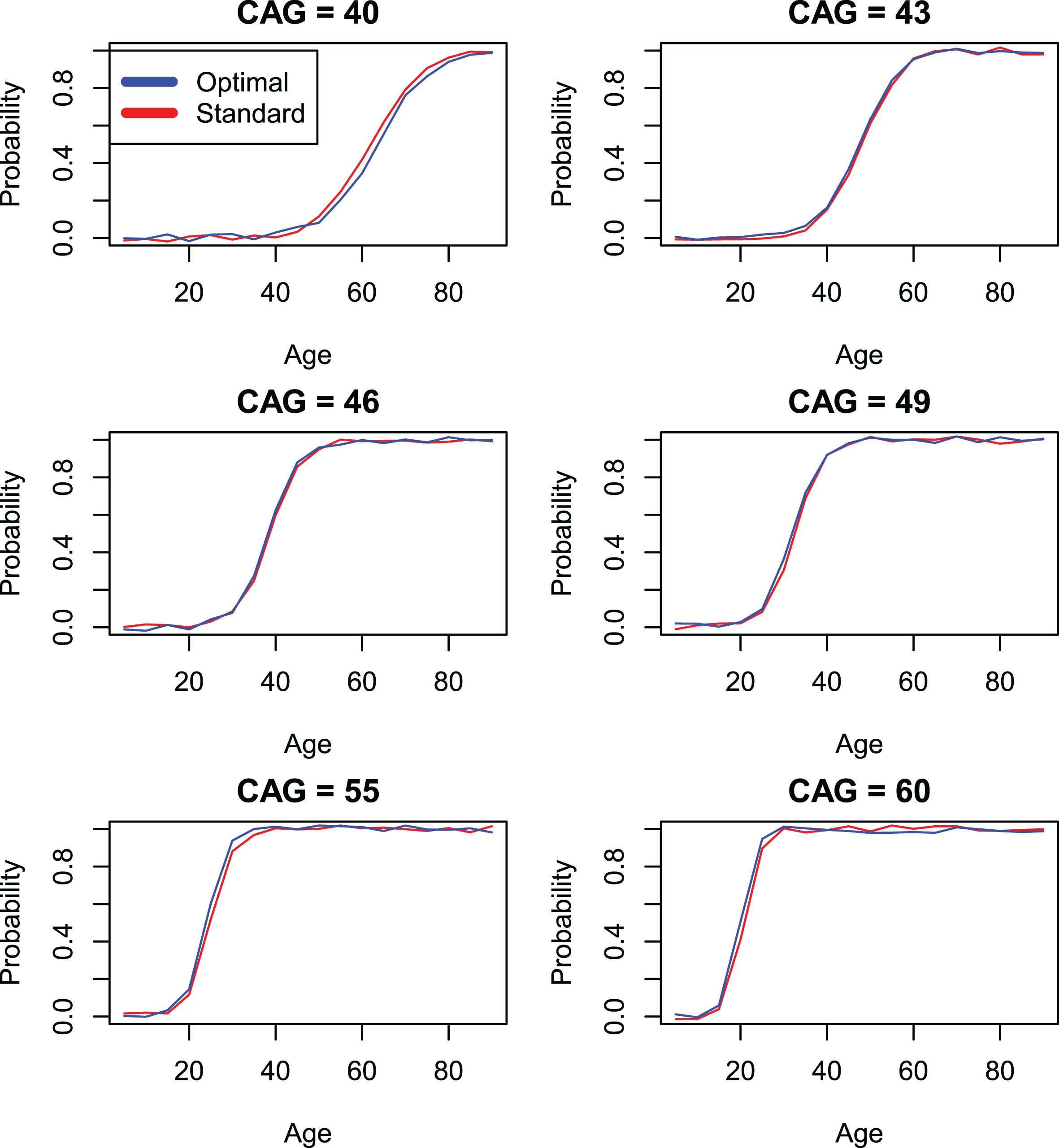
Comparison of standard CAP score models with individually optimized models (models 4 and 3) by onset variable sxrater.

Fig. 3

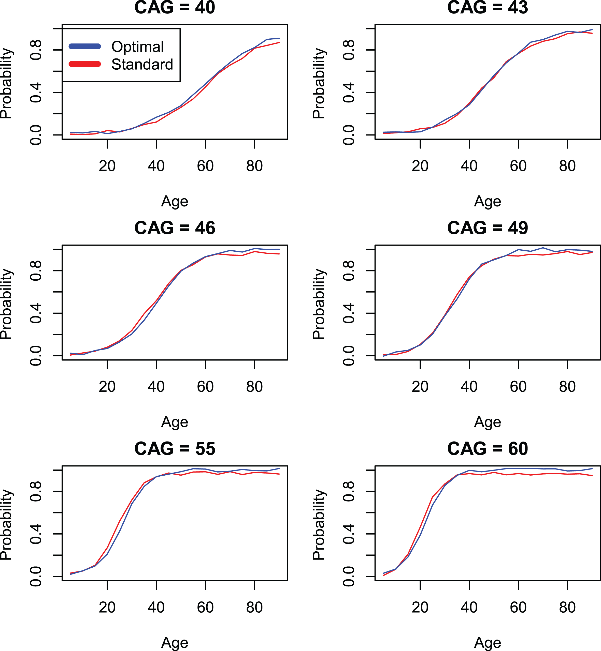
Comparison of standard CAP score models with individually optimized models (models 4 and 3) by onset variable ccdepage.

Validating the onset model

Figures 4 and 5 compare the standard CAP score AO model (for all 13 onset measures) with the model of [19]. Agreement is generally good, except for the psychiatric onset variables that would be expected to follow a different pattern. We note that our preferred onset variable (time-to-diagnosis or hddiagn) produces slightly later AOs than does the model of [19]. In contrast, the model for DCL4 shows a slightly earlier onset than does the model of [19]. It is important to note that the model of [19] was fit to data described in that publication, not to the Enroll data. This data was most similar to the variables sxsubj, sxfam, and sxrater in our data set. The model of [19] was never intended to be used in predicting psychiatric onset. As a result, the large discrepancies in Fig. 5 represent differences in the underlying distributions rather than differences in the modeling procedures.

Fig. 4

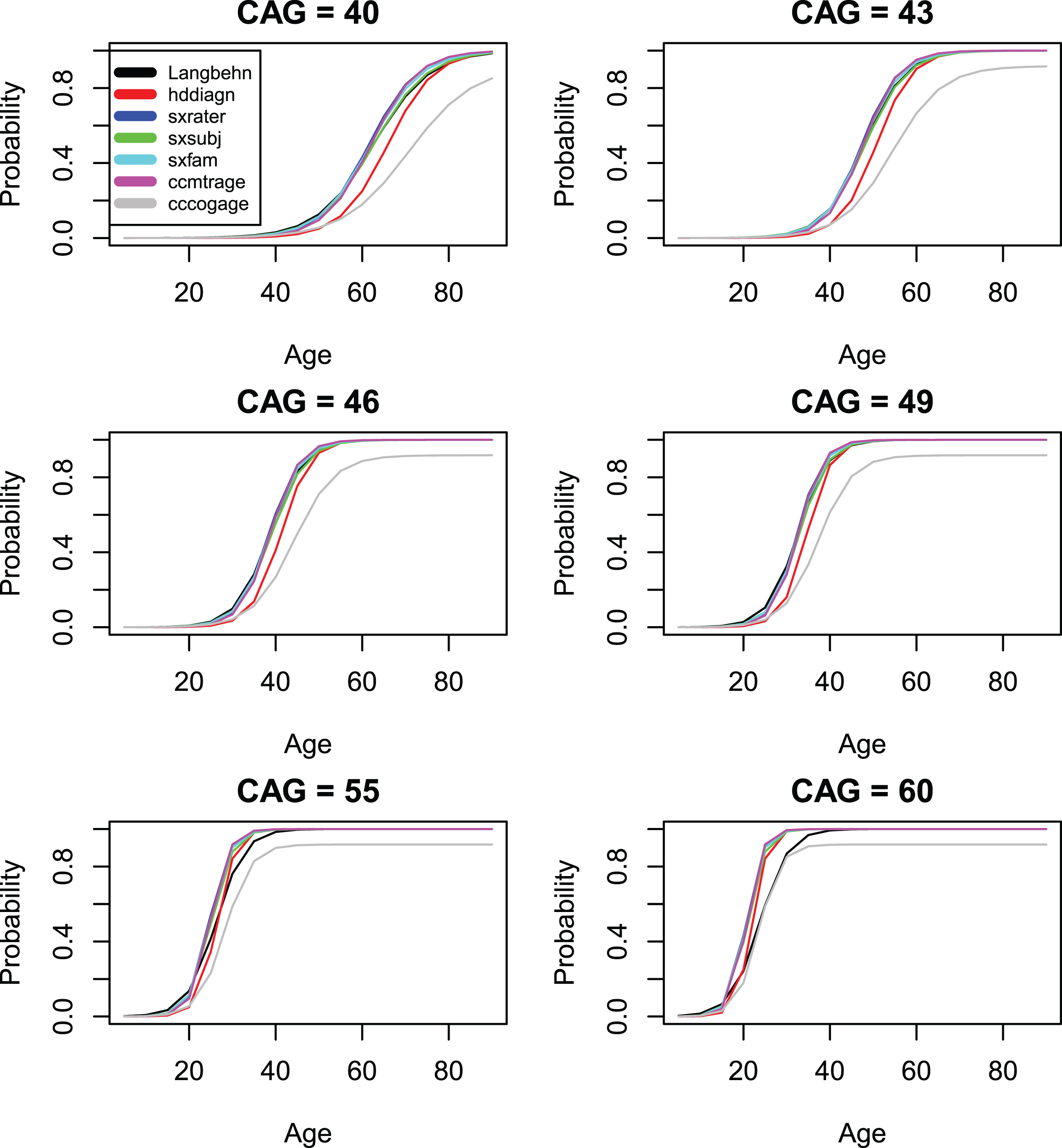
Comparison of standard CAP score models with the model of [19] (onset variables 1–6).

Fig. 5

Comparison of standard CAP score models with the model of [19] (onset variables 7–13).

Figures 6 through 8 compare survival plots for the CAP score Model 4 compared with non-parametric survival curves for each onset variable. The nonparametric estimates of the survival curves are presented in the form of probability distributions together with upper and lower bounds for the 95% confidence interval based on the cumulative hazard function. The figures show that survival plots from the CAP score survival models are closely matched by nonparametric survival plots for the AO variables of Table 2. This provides evidence that the assumed logistic form of Equation 7 is, to a very good approximation, correct. A more detailed treatment of these issues appears in section 6 of the Supplementary Material where the plots of Figs. 6 –8 are presented separately for each value of CAG length between 40 and 56. In our view, all the above analyses produce plots that are remarkably close to the original logistic functional form. This is particularly true when the most common CAG lengths are considered (i.e., CAG lengths between 40 and 50). For CAG lengths larger than 50, the evident lack of fit may be ascribed to sample sizes that are too small for accurate non-parametric analysis.

Fig. 6

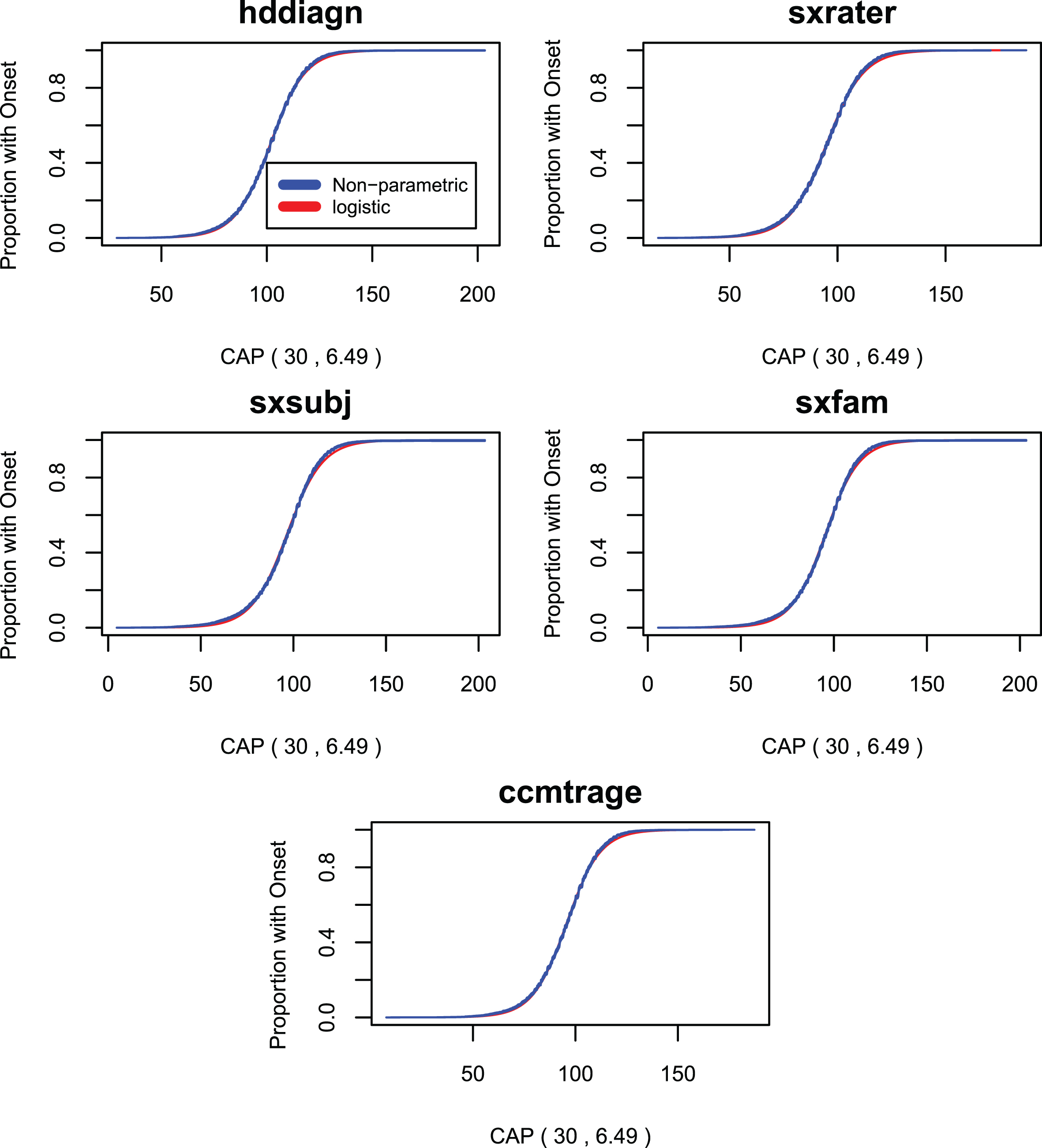
Survival curves for the standard CAP score model compared with non-parametric survival curves onset variables 1–5.

Fig. 7

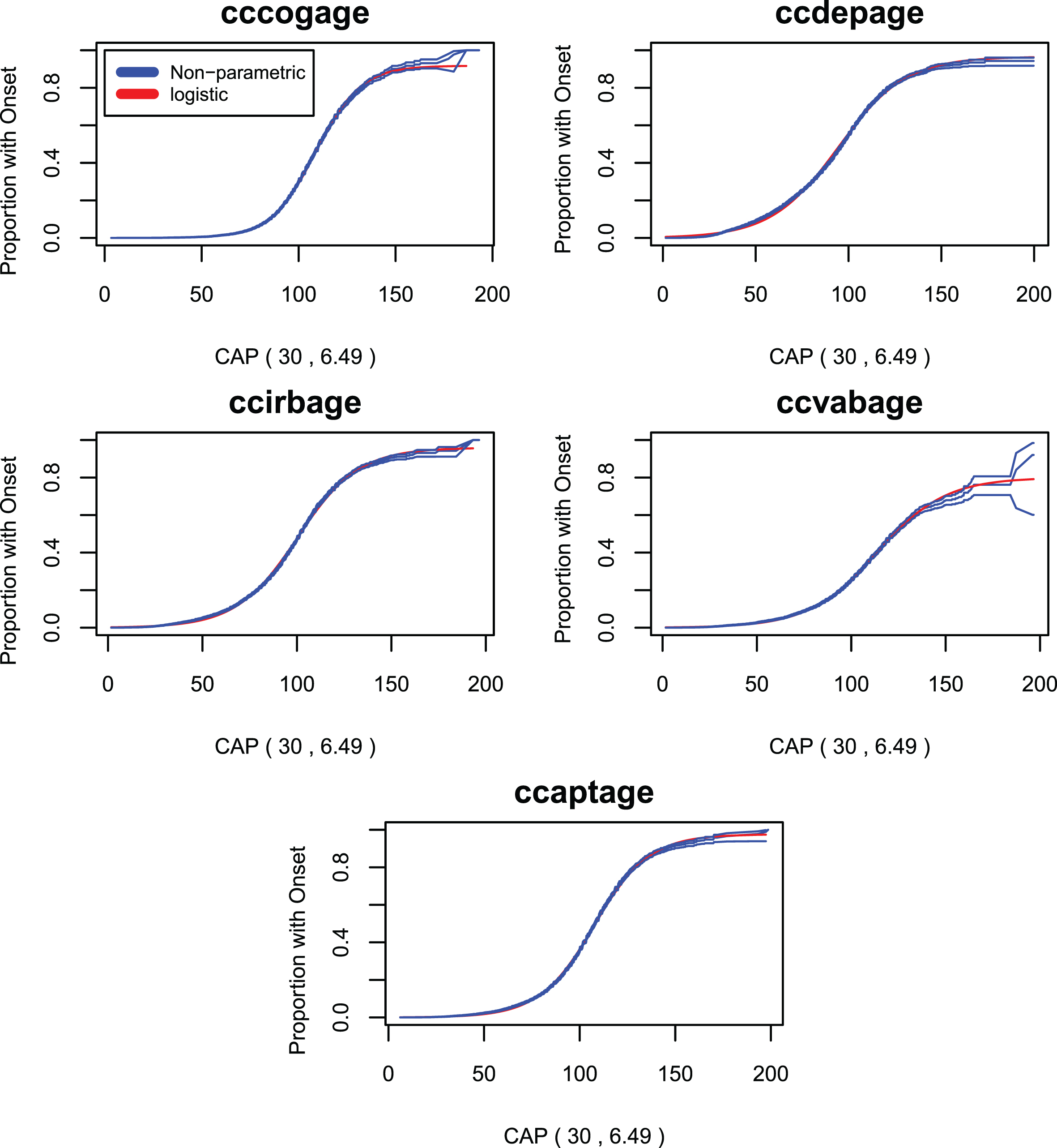
Survival curves for the standard CAP score model compared with non-parametric survival curves onset variables 6–10.

Fig. 8

Survival curves for the standard CAP score model compared with non-parametric survival curves onset variables 11–13.

Figures 9 to 11 present plots of the correlation of (CAG - L) AO with CAG length vs. L for each AO variable. These curves are seen to cross the x-axis at values of L which are remarkably close to the optimal values from Table 6: this suggests that imposing the condition that CAP at onset is uncorrelated with CAG length is sufficient to determine the value of the parameter L. In addition, these plots show that, when evaluated at AO, CAP scores with L = 33.66 and L = 35.5 have markedly higher correlations with CAG length than do CAP scores with L = 30. Only uncensored observations are used in these plots.

Fig. 9

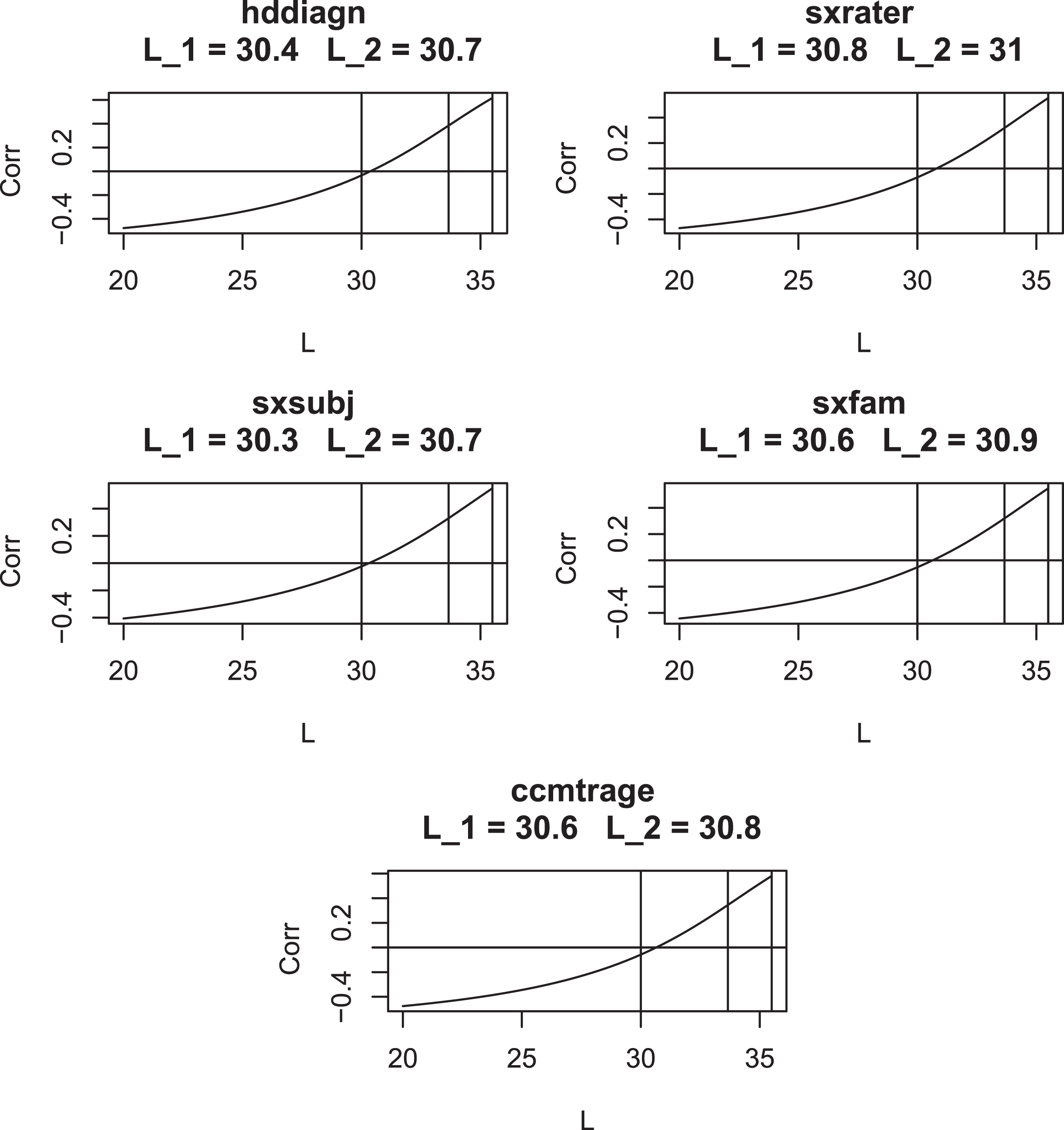
Correlation of (CAG –L) AO with CAG length for various values of L for AO Variables 1–5. Vertical lines are drawn at L = 30, L = 33.66, and L = 35.5. L1 is the value of L where the graph crosses the x-axis. L2 is taken from Table 5.

Fig. 10

Correlation of (CAG –L) AO with CAG length for various values of L for AO Variables 6–10. Vertical lines are drawn at L = 30, L = 33.66, and L = 35.5. L1 is the value of L where the graph crosses the x-axis. L2 is taken from Table 5.

Fig. 11

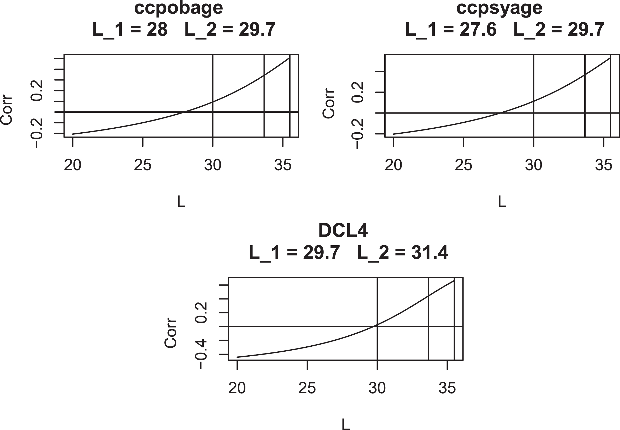
Correlation of (CAG –L) AO with CAG length for various values of $L$ for AO Variables 11–13. Vertical lines are drawn at L = 30, L = 33.66, and L = 35.5. L1 is the value of L where the graph crosses the x-axis. L2 is taken from Table 5.

Section 4 of the Supplementary Material provides Bayesian confidence intervals for the parameter estimates of the individually optimized model (Model 3) for each onset variable. Of particular interest is the observation that the 95% confidence intervals for α are always bounded well away from 0: this removes any doubt that might remain regarding the effect of CAG length on each and all of the onset variables.

For completeness, Section 5 of the Supplementary Material provides Bayesian confidence intervals for the parameters of the Standard CAP score models.

DISCUSSION

The literature on AO models in HD has now become extensive (see, for example the reviews in [29] and [30]). We do not claim that the onset models presented here have any advantages over existing models except insofar as they isolate the effect of exposure to mHTT (as measured by CAP score) on the prediction of onset. Indeed, it has been shown in [31] and elsewhere that the use of dynamic measures of clinical status can improve the prediction of onset events, over and above what can be done using age and CAG length alone. It was not our intention to advance a particular onset model. Rather our goal is to use the above onset models to create a rational method for standardizing the CAP score.

Specifically, we seek to carry out this standardization at this time in order to

Avoid confusion when comparing CAP scores across studies

Update previous justifications of the CAP score using new data

Provide users with an operational definition of the toxicity that is measured by CAP

Elucidate the close connection between AO and CAP

Provide a baseline landmark against which models for the effect of somatic expansion on AO can be compared.

On balance, and in view of the above rationale, we feel that our recommendation for the use of L = 30 and K = 6.49 has held up well. At the same time, we realize that some reservations and objections may remain which we will address below.

To begin, we realize that onset (however it is defined) is not an event that occurs at a specific point in time. Onset differs in this respect from archetypal events (like death) that are the basis for time-to-event (or survival) analysis. Nonetheless, we feel that the literature on AO has made useful contributions to our understanding of the HD process and hope that the current work will extend this tradition. In our view, the most promising practical application of the current study lies in facilitating the use of the CAP score in the prediction of continuous disease state variables. Such predictions may be useful in the analysis of natural history studies and in the planning of clinical trials of potentially disease-modifying treatments. In the latter case, the CAP score’s connection with etiology of HD may make it a useful tool for quantifying a hypothesized drug effect; that is, the effect of a hypothetical drug may be likened to the reduction of CAG length in Equation 7 by a given number of repeats.

We would also like to draw attention to our demonstration that the distribution of CAP, evaluated at age-of-onset, is independent of CAG length and the related non-parametric method for determining L. While this observation has a somewhat technical sound to it, we believe that it is important in practice. In particular, we have shown that with values of L in common use (i.e., L = 33.66 or L = 35.5), CAP(AO) has a significant correlation with CAG length. This raises the possibility that the use of CAP scores in regression models with the above values of L could introduce spurious correlations with CAG length. In addition, CAP scores that have CAG dependent distributions when evaluated at AO are, by definition, of questionable validity as measures of the cumulative toxicity of mutant huntingtin.

We would also like to distinguish our work from [32], which elucidates the role of CAG repeats in long term progression of HD without attempting to incorporate this role into an exposure-response model as is done by the CAP score. Also of interest is [33], which demonstrates a role for the CAG dependence of disease progression after the onset event. This contradicts the time-to-event analysis of [34], which argued that the length of the interval between onset and death is independent of CAG length. In our view, the nature of CAG length dependence is altered, but not eliminated, by the onset event. In this respect we view the role of natural aging mechanisms, independent of but complementary to CAG induced toxicity, as a causal factor in the etiology of cognitive and motor decline in HD [35, 36]. It is also likely that disease stage will have an independent effect on toxicities leading to disease progression. While natural aging may have a causal effect on HD onset, it would be very difficult to estimate such an effect due to the sparsity of data on false “onset” in individuals who do not carry the HD mutation. The situation is quite different for continuous measures of motor and cognitive status which are routinely observed in both HDGECs and healthy controls making controlling for normal aging possible and, arguably, necessary.

The full promise of exposure-response models in HD, however, cannot be realized without addressing the role of somatic expansion in HD pathology [37 –39]. Under somatic expansion, CAG length becomes a time varying quantity CAG(t). By analogy with Equation 7, we can define a CAP score onset model that takes somatic expansion into account. Such a model can be formulated a toxicity onset model with $\begin{matrix} TOX = {(CAG (t) - L)}_{+} \\ AUC = \int_{0}^{T} (CAG (t) - L) dt \end{matrix}$ (14) leading to a definition of CAP_se of the form $CA P_{se} = \int_{t = 0}^{AGE} \frac{{(CA G_{se} (t) - L)}_{+} dt}{K}$ (15) where CAG_se(t) is an estimate of some functional (e.g., the mean, median, 95th percentile) of the distribution of somatically expanded CAG lengths, as would occur in the striatum or other affected regions. One possible form of a model leading to such and estimate is $CA G_{se} (t) = (CAG - C_{0}) exp (λ t) + C_{0}$ where CAG is as in Equation 1, λ is an expansion rate constant which could itself be modeled as a function of genetic modifiers like those identified in [40], and C₀ is a parameter indicating the minimum CAG length at which somatic expansion occurs. Still more complex models in which CAG(t) in Equation 14 is allowed to vary in size between cells (as it does in [37 –39]) can also be considered, in which case the event of interest would relate to neuronal death or the shrinkage of the neuropils of a select class of cells. Models of all of the above types are currently under study but beyond the scope of the current paper. That said, one reason for our interest in the standard CAP score of Equation 1 is that it can serve as a source of null hypotheses against which models based on 15 can be evaluated. This research is ongoing with the view of providing an alternative elaboration of the two component sequential model for HD pathogenesis advocated in [41].

Some may be concerned by our treatment of CAP score as a modified survival time. One referee has pointed out that this practice is analogous to the way quality adjusted survival time (QAST) is handled in the oncology literature [42, 43] where it is acknowledged that the non-parametric analysis of such modified survival time variables requires special treatment to avoid the effects of induced informative censoring. While we acknowledge some similarities between QAST and CAP, we feel that the cases differ in some important respects. First, while QAST includes information gathered from each subject that is collected separately from time, the modifications of time implied by CAP includes only information on CAG length which is fixed from conception for each individual and is related to disease progression as a cause rather than an effect. Indeed, in the toxicity onset formulation (with and without somatic expansion), both TOX and AUC are parametric functions of time. In addition, when differentiation of F in Equation 4 is carried out, it is done with respect to T not AUC leading to models in which censoring is defined in terms of time not CAP. As a second point, CAP lends itself more than QAST to a grouping strategy. In particular, we performed analyses separately for each of the 17 CAG lengths (40–56) as we report in section 6 of the Supplementary Material. These analyses are relevant in that they argue not only for the correctness of the logistic functional form of the survival function but also for the proposition that this functional form applies regardless of CAG length. What is more, while we believe that the analysis of Figs. 6 through 8 are valid, there is no doubt that the analyses based on the above grouping strategy are valid, as the re-scaling factor for time which they employ reduces to a constant in each analysis. In sum, for the reasons given above, we argue that the analytic procedures of [42] and [43] are not needed for the non-parametric analysis of CAP or (arguably) CAP_se.

Some may also be uncomfortable with taking L = 30 as a lower limit for CAG induced toxicity. As has already been mentioned CAG = 36 is the lowest value for which definitive diagnosis of HD has been made. That said some authors have suggested that some symptoms, similar to those of HD, have been observed for individuals with CAG lengths in the intermediate range of 27–35 repeats [44, 45]. It is interesting that the psychiatric symptoms so observed appear to be related to the psychiatric onsets which we found to follow a different distributional form compared to the more traditional motor symptoms. We note that our study differed from [44] in that cognitive onset also followed an altered pattern. It is also, of course, possible that some toxicity might be occurring in some individuals without producing any overt signs or symptoms.

Finally, we have observed from our analyses of both AO and continuous outcome measures, and from the forms of Equations 1 and 15 that

Ignoring the effect of normal aging, when it is present, is likely to decrease the estimated value of L

Even modestly positive values of λ in Equation 15 will tend to increase the associated estimate of L.

The upshot of the above considerations is that, at this time, L = 30 should be treated as a convenient, conventional, standardizing value and not a firmly established, physiologically-based estimate.

Footnotes

ACKNOWLEDGMENTS

Data used in this work were generously provided by the participants in the Enroll-HD study and made available by CHDI Foundation, Inc. Enroll-HD is a clinical research platform and longitudinal observational study for Huntington’s disease families intended to accelerate progress towards therapeutics; it is sponsored by CHDI Foundation, a nonprofit biomedical research organization exclusively dedicated to collaboratively developing therapeutics for HD. Enroll-HD would not be possible without the vital contribution of the research participants and their families. The individuals who contributed to the collection of the Enroll-HD data are also gratefully acknowledged; see

CONFLICT OF INTEREST

John H. Warner, Jennifer Ware, and Cristina Sampaio are employed by CHDI Management as advisors to CHDI Foundation, as was Amrita Mohan during this analysis. Jeffrey D. Long, James A. Mills, and Douglas R. Langbehn receive research funding from CHDI Foundation. In addition, Dr. Langbehn reports personal consulting fees and non-financial support from Voyager Therapeutics, personal consulting fees from Novartis, personal consulting fees from uniQure, personal consulting fees from Takeda, and personal consulting fees from AskBio, all outside the submitted work. Dr. Long is a paid committee member for F. Hoffmann-La Roche Ltd and uniQure biopharma B.V., and he is a paid consultant for PTC Therapeutics Inc, Remix Therapeutics Inc, Spark Therapeutics Inc, Triplet Therapeutics Inc, and Wave Life Sciences USA Inc. James Mills is a paid consultant for PTC Therapeutics Inc. and Triplet Therapeutics Inc.

The supplementary material is available in the electronic version of this article: .

References

Bates

, Dorsey

, Gusella

, Hayden

, Kay

, Leavitt

, et al. Huntington disease. Nat Rev Dis Primers. 2015;1:15005.

Jones

, Hughes

. Pathogenic mechanisms in Huntington’s disease. Int Rev Neurobiol. 2011;98:373–418.

Mangiarini

, Sathasivam

, Seller

, Cozens

, Harper

, Hetherington

, et al. Exon 1 of the HD gene with an expanded CAG repeat is sufficient to cause a progressive neurological phenotype in transgenic mice. Cell. . 1996;87(3):493–506.

Rué

, Bañez-Coronel

, Creus-Muncunill

, Giralt

, Alcalá-Vida

, Mentxaka

, et al. Targeting CAGrepeat RNAs reduces Huntington’s disease phenotype independently ofhuntingtin levels. J Clin Invest.. 2016;126(11):4319–30.

Warner

, Sampaio

. Modeling variability in the progression of Huntington’s disease a novel modeling approach applied to structural imaging markers from TRACK-HD. CPT Pharmacometrics Syst Pharmacol. 2016;5(8):437–45.

, Faria

, Younes

, Mori

, Brown

, Johnson

,et al. Mapping the order and pattern of brain structural MRI changes using change-point analysis in premanifest Huntington’s disease. Hum Brain Ma. 2017;38(10):5035–50.

Reading

, Yassa

, Bakker

, Dziorny

, Gourley

, Yallapragada

, et al. Regional white matter change in pre-symptomatic Huntington’s disease: a diffusion tensor imaging study. Psychiatry Res. 2005;140(1):55–62.

Fazio

, Fitzer-Attas

, Mrzljak

, Bronzova

, Nag

, Warner

, et al. PET molecular imaging of phosphodiesterase 10A: an early biomarker of Huntington’s disease progression. Mov Disord. 2020;35(4):606–15.

Ross

, Aylward

, Wild

, Langbehn

, Long

, Warner

, et al. Huntington disease: natural history, biomarkers and prospects for therapeutics. Nat Rev Neurol. 2014;10(4):204–16.

10.

Byrne

, Rodrigues

, Blennow

, Durr

, Leavitt

, Roos

RAC

, et al. Neurofilament light protein in blood as a potential biomarker of neurodegeneration in Huntington’s disease: a retrospective cohort analysis. Lancet Neurol. 2017;16(8):601–9.

11.

Zhang

, Long

, Mills

, Warner

, Lu

, Paulsen

. Indexing disease progression at study entry with individuals at-risk for Huntington disease. Am J Med Genet B Neuropsychiatr Genet. 2011;156b(7):751–63.

12.

Mohan

, Sun

, Ghosh

, Li

, Cheng

, Hu

, et al. A unified staging system for prodromal and manifest Huntington’s disease [abstract]. Mov Disord. 2019;34(suppl 2).

13.

Wells

, Ashizawa

. Genetic instabilities and neurological diseases. Oxford: Elsevier2006.

14.

Paulsen

, Long

, Johnson

, Aylward

, Ross

, Williams

, et al. Clinical and biomarker changes in premanifest Huntington disease show trial feasibility: a decade of the PREDICT-HD Study. Front Aging Neurosci. 2014;6:78.

15.

Paulsen

, Long

, Ross

, Harrington

, Erwin

, Williams

, et al. Prediction of manifest Huntington’s disease with clinical and imaging measures: a prospective observational study. Lancet Neurol. 2014;13(12):1193–201.

16.

Penney

Jr . , Vonsattel JP, MacDonald ME, Gusella JF, Myers RH. CAG repeat number governs the development rate of pathology in Huntington’s disease. Ann Neurol. 1997;41(5):689–92.

17.

Tabrizi

, Scahill

, Owen

, Durr

, Leavitt

, Roos

, et al. Predictors of phenotypic progression and disease onset in premanifest and early-stage Huntington’s disease in the TRACK-HD study: analysis of 36-month observational data. Lancet Neurol. 2013;12(7):637–49.

18.

Paulsen

, Hayden

, Stout

, Langbehn

, Aylward

, Ross

, et al. Preparing for preventive clinical trials: the Predict-HD study. Arch Neurol. 2006;63(6):883–90.

19.

Langbehn

, Brinkman

, Falush

, Paulsen

, Hayden

. A new model for prediction of the age of onset and penetrance for Huntington’s disease based on CAG length. Clin Genet. 2004;65(4):267–77.

20.

Landwehrmeyer

, Fitzer-Attas

, Giuliano

, Gonçalves

, Anderson

, Cardoso

, et al. Data analytics from Enroll-HD, aglobal clinical research platform for Huntington’s disease. MovDisord Clin Pract.. 2017;4(2):212–24.

21.

Enroll-HD-PDS5-Overview [press release]. New York: CHDI Foundation, Inc.2020.

22.

Kalbfleisch

, Prentice

. The statistical analysis of failure time data. New York: John Wiley & Sons, Inc.; 2011.

23.

Team SD. Stan Modeling Language: User’s Guide and Reference Manual: CreateSpace Independent Publishing Platform; 2012.

24.

Team SD. RStan: the R interface to Stan. R package version 2.21.1.2020.

25.

Therneau

, Lumley

. Package ‘survival’. R Top Doc. 2015;128(10):28–33.

26.

Turnbull

. Nonparametric estimation of a survivorship function with doubly censored data. J Am Stat Assoc. 1974;69(345):169–73.

27.

Team RC. R: A language and environment for statistical computing, R Foundation for Statistical Computing; 2017.

28.

Enroll-HD Team. Enroll-HD: Periodic Dataset 4. A user guide to the clinical datasets and biosamples available from Enroll-HD2018. Available from: https://www.enroll-hd.org/enrollhddocuments/2018-10-R1/Enroll-HD-User-Guide-2018-10-R1.pdf

29.

Langbehn

, Hayden

, Paulsen

. CAG-repeat length and the age of onset in Huntington disease (HD): a review and validation study of statistical approaches. Am J Med Genet B Neuropsychiatr Genet;2010;153b(2):397–408.

30.

Garcia

, Marder

, Wang

. Statistical modeling of Huntington disease onset. Handb Clin Neurol. 2017;144:47–61.

31.

Long

, Langbehn

, Tabrizi

, Landwehrmeyer

, Paulsen

, Warner

, et al. Validation of a prognostic index for Huntington’s disease. Mov Disord. 2017;32(2):256–63.

32.

Langbehn

, Stout

, Gregory

, Mills

, Durr

, Leavitt

, et al. Association of CAG repeats with long-term progression in Huntington disease. JAMA Neurol. 2019;76(11):1375–85.

33.

Langbehn

. Longer CAG repeat length is associated with shorter survival after disease onset in Huntington disease. Am J Hum Genet. 2022;109(1):172–9.

34.

Keum

, Shin

, Gillis

, Mysore

, Abu Elneel

, Lucente

,et al. The HTT CAG-expansion mutation determines age at death but not disease duration in Huntington disease. Am J Hum Genet. 2016;98(2):287–98.

35.

Machiela

, Southwell

. Biological aging and the cellular pathogenesis of Huntington’s disease. J Huntingtons Dis. 2020;9(2):115–28.

36.

Mills

, Long

, Mohan

, Ware

, Sampaio

. Cognitive and motor norms for Huntington’s Disease. Arch Clin Neuropsychol. 2020;35(6):671–82.

37.

Benn

, Gibson

, Reynolds

. Drugging DNA damage repair pathways for trinucleotide repeat expansion diseases. J Huntingtons Dis. 2021;10(1):203–20.

38.

Higham

, Morales

, Cobbold

, Haydon

, Monckton

. High levels of somatic DNA diversity at the myotonic dystrophy type 1 locus are driven by ultra-frequent expansion and contraction mutations. Hum Mol Genet. 2012;21(11):2450–63.

39.

Kaplan

, Itzkovitz

, Shapiro

. A universal mechanism ties genotype to phenotype in trinucleotide diseases. PLoS Comp Biol. 2007;3(11):e235.

40.

Identification of genetic factors that modify clinical onset of Huntington’s disease. Cell. 2015;162(3):516–26.

41.

Gusella

, Lee

, MacDonald

. Huntington’s disease: nearly four decades of human molecular genetics. Hum Mol Genet. 2021;30(R2):R254–r63.

42.

Zhao

, Tsiatis

. A consistent estimator for the distribution of quality adjusted survival time. Biometrika. 1997;84(2):339–48.

43.

Zhao

, Tsiatis

. Efficient estimation of the distribution of quality-adjusted survival time. Biometrics. 1999;55(4):1101–7.

44.

Killoran

, Biglan

, Jankovic

, Eberly

, Kayson

, Oakes

,et al. Characterization of the Huntington intermediate CAG repeat expansion phenotype in PHAROS. Neurology.2013; 80(22):2022–7.

45.

Semaka

, Hayden

. Evidence-based genetic counselling implications for Huntington disease intermediate allele predictive test results. Clin Genet. 2014;85(4):303–11.